Two Dimensional Model for Backwater Geomorphology: Darby Creek, PA


Civil and Environmental Engineering Department, Villanova University, Villanova, PA 19085, USA
*
Author to whom correspondence should be addressed.
Water 2019, 11(11), 2204; https://doi.org/10.3390/w11112204
Submission received: 29 August 2019
/
Revised: 10 October 2019
/
Accepted: 15 October 2019
/
Published: 23 October 2019
(This article belongs to the Section Hydraulics and Hydrodynamics)
Abstract
:Predicting morphological alterations in backwater zones has substantial merit as it potentially influences the life of millions of people by the change in flood dynamics and land topography. While there is no two-dimensional river model available for predicting morphological alterations in backwater zones, there is an absolute need for such models. This study presents an integrated iterative two-dimensional fluvial morphological model to quantify spatio-temporal fluvial morphological alterations in normal flow to backwater conditions. The integrated model works through the following steps iteratively to derive geomorphic change: (1) iRIC model is used to generate a 2D normal water surface; (2) a 1D water surface is developed for the backwater; (3) the normal and backwater surfaces are integrated; (4) an analytical 2D model is established to estimate shear stresses and morphological alterations in the normal, transitional, and backwater zones. The integrated model generates a new digital elevation model based on the estimated erosion and deposition. The resultant topography then serves as the starting point for the next iteration of flow, ultimately modeling geomorphic changes through time. This model was tested on Darby Creek in Metro-Philadelphia, one of the most flood-prone urban areas in the US and the largest freshwater marsh in Pennsylvania.
1. Introduction
The majority of the world’s population lives near the coast [1], typically in urban population hubs [2,3,4,5], often close to the receiving waters. Due to climate change and population growth, coastal zone flooding is projected to have an increased adverse impact on the global economy [6]. Further, these at-risk coastal areas host critical ecosystems. Understanding the fluvial morphodynamics of this zone is important to mitigate the impacts of floods on the ever-growing urban coastal populations and can aid in protecting vital coastal zone ecosystems. In addition to coastal areas, dammed rivers are also subjected to backwater (BW) conditions. Dams act as blocks on rivers and by forming backwater conditions, change the water surface profile upstream [7,8,9,10,11]. By 2018, there were more than 59,000 large dams built all around the world [8]. In US itself, there are more than 2 million low-head dams [10] which alter the hydraulics, sediment erosion and deposition regime of the rivers due to BW conditions [9]. However, the spatial impacts of such dams on morphological alterations in rivers are highly unexplored [10].
A major challenge of understanding the morphodynamics of this zone is the presence of BW hydraulics. This condition can occur as a river joins a body of standing water (e.g., ocean, lake, and dam reservoir), where the water surface elevation at the river mouth varies depending upon the water surface elevation (WSE) of the standing water downstream. The downstream standing water forces an upstream adjustment in the river, causing the WSE to back up towards the upstream. The depth of the river increases gradually upstream to form a smooth transition between a quasi-normal flow and standing water, forcing an alteration of the hydraulic conditions. The segment of the river affected by this response—which might exceed hundreds of kilometers in low slope rivers—is called the backwater zone [12].
The shift in BW hydraulics causes the water surface slope to decrease independent of the bed slope, resulting in a gradual longitudinal alteration of the flow depth and velocity [13]. The vertical velocity distribution in BW conditions is less divergent compared to the one in a uniform flow [14]. These changes in the hydraulics of the vertical and horizontal flow velocity in BW zones consequently alter the sediment transport processes.
Current approaches to BW in morphological studies are primarily based on either measured or estimated hydraulic parameters coupled with the estimated sediment transport [9,11,15,16,17,18,19,20,21]. The studies of sediment transport in BW conditions are scarce due to the complex dynamics of the sediment transport in BW zones and the lack of field-measured data. The presence of the BW complicates different types of hydrometric measurements including the water surface slope, velocity, and discharge [19]. A lack in measured data is even more severe for transitional areas where the flow state changes from normal to a gradually varied flow [18]. Nittrouer et al. used measured cross sections in the lower Mississippi River to back calculate velocity, shear stress and sediment discharge [22]. They concluded that where the flow transitions to the BW zone, the cross-sectional area increases in the downstream in low-moderate flows, resulting in a decrease in shear stress and sediment transport. This is in line with the findings of Lu et al. [18] and Liro [9]. Conversely, during high flows, the water surface elevation is drawn down (M2 profile in mild slopes [23]) to match the water surface of the standing water downstream. Therefore, the cross sectional area decreases downstream and results in a substantial increase in shear stress and sediment transport [24,25,26]. On the experimental side, Jin et al. studied shear stress in BW conditions based on flume measurements. They showed that increases in depth (y) relative to normal depth (yn) (increases in y/yn at ratios of higher than one) in BW conditions decreases the shear stress exponentially [14]. Zhang et al. used a mathematical model to show that in BW conditions, the shear velocity and consequently the shear stress decrease with an increase in the water depth when the discharge and slope are fixed. They concluded that in BW flow, lateral momentum flux causes the Reynolds shear stress term (and shear stress eventually) in the momentum equation to deviate from the one in the normal flow [27]. This suggests that for the depths above normal, the shallower parts of the river in BW conditions are more likely to experience erosion.
In addition to local alterations in shear stress due to depth variations, the difference in the rate of flow deceleration affects the spatial distribution of erosion and deposition. In low-flow discharges and transition zones from normal to a gradually varied flow, the deceleration of the flow (M1 profile in mild slopes [23]) enhances the sediment deposition [28]. The variations in velocity distribution, shear stress and sediment transport rate in the BW zone, which differ from the ones in the normal flow, complicate the prediction of the morphological alterations in the river [9,14,18,27]. Moreover, the extent of the transported sediment such as the location, volume, and duration of bed material deposition in the BW is to some extent unknown [22,27].
Here, this study presents a 2D analytical morphological model which was applied to quasi-normal flow transitioning into BW flow, using Darby Creek, PA as a case study. The modelling of the spatio-temporal dynamics of the sediment in BW river conditions is key to understanding the morphodynamic processes of the river and land evolution. Although there are multiple hydraulic models available for predicting the water surface profile in gradually varied flow zones [17,18], the 2D morphological models currently available for BW and transitional zones are not well known. This paper presents an integrated model to predict the spatio-temporal fluvial morphological alterations in BW and the transition into the BW zone. To accomplish this, a 1D gradually varied flow model (for BW and transition zones) was integrated with a 2D normal flow model (for quasi normal zone) to generate the water surface profile. Ultimately, an analytical 2D morphological model was developed to estimate the shear stress and sediment transport rate over the computational domain. The unique 1D model captures the change in WSE across the BW transition, which allows the 2D model to capture the sediment flux. The current approaches in geomorphological assessment in the BW zone are mainly limited to either a few years-worth or thousands years of geomorphic changes [29,30,31,32,33,34,35,36,37,38]. In contrast, the presented integrated model builds on the existing body of knowledge in geosciences which can predict geomorphological alterations in the BW zone of the rivers over a short to intermediate time scale applicable to civil engineering applications.
2. Materials and Methods
2.1. Study Area
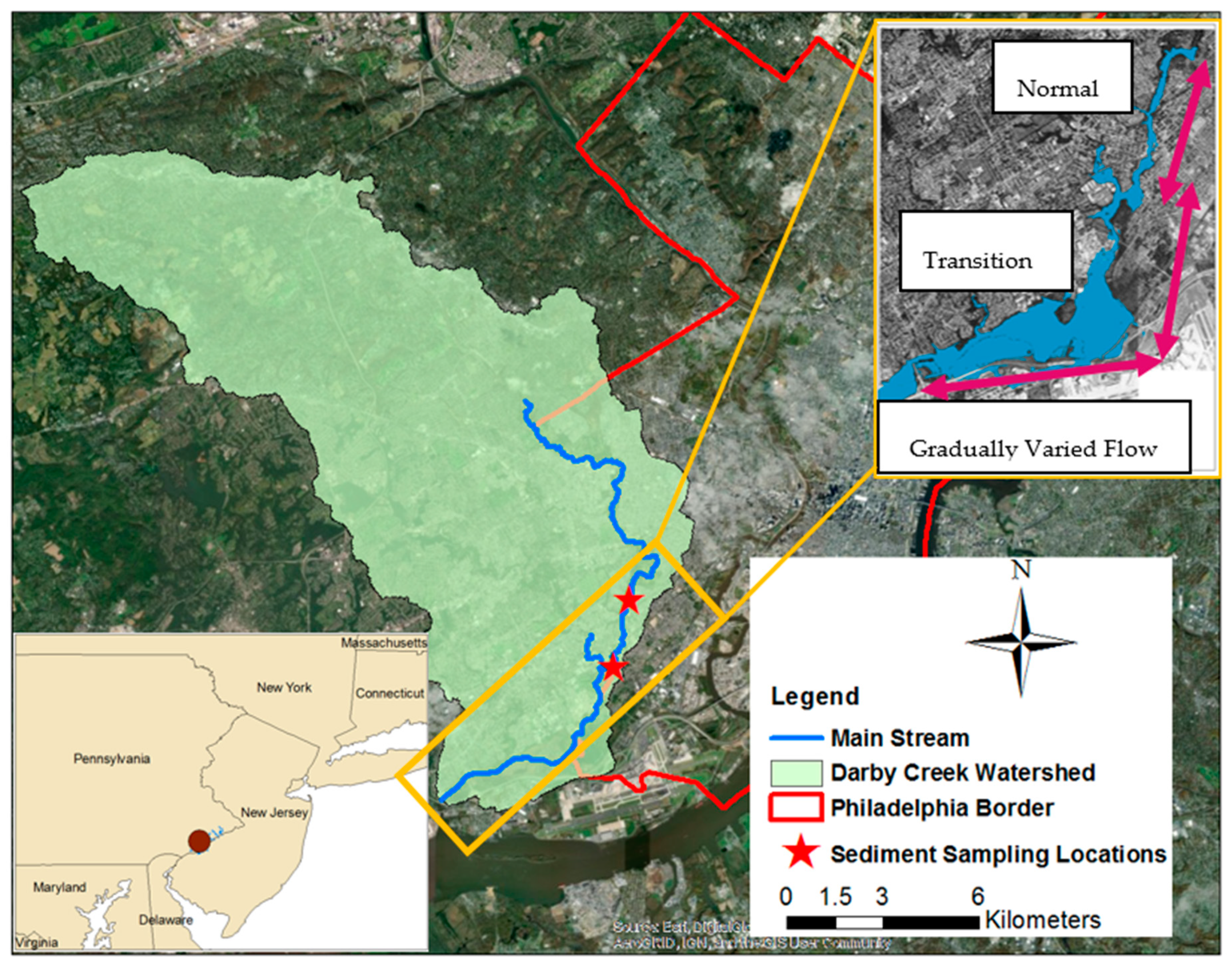
The study area for this work is in the lower part of the Darby Creek, near Philadelphia, PA (Figure 1). The creek with its alluvial deposits passes through a fully urbanized floodplain subject to frequent flooding [39] where the flashiness of the flow has the potential to impact the lives of local residents significantly [40]. The segment of the river focused on in this study runs from Mt. Moriah Cemetery (upstream) to the confluence with the Delaware River (downstream), reaching to a length of approximately 15 river kilometers (rkm). The Delaware River at the downstream imposes BW conditions to the lower part of the creek. The flow regime of the upper segment of the creek can be considered normal (quasi-normal), while in the lower part the flow regime changes to a gradually varied flow (Figure 1). Approximately 7 rkm of the lower part of the creek is estimated to be in BW conditions.
The channel and floodplain evolution prediction is currently of great concern for Darby Creek. In addition to being flood prone, as a wetland in close proximity to urban Philadelphia, it plays an important environmental role [41]. The creek flows into the biggest fresh water marsh zone in Pennsylvania, and it provides a unique environment for different species of plants and animals. The marsh area is known as the Heinz National Wildlife Refuge [42].
2.2. Integrated Model
An integrative-iterative modeling approach is proposed to simulate morphological alterations in BW conditions. The model uses a suite of observational data coupled with several models that run in an iterative process. The first phase of the model requires data collection and integration. To accomplish this, the first step is to identify the BW, normal, and transitional zones. Then, the different hydraulic models are used to generate WSE for BW and normal zones separately. The following three steps define the method that was developed to estimate WSE for the whole domain:
- (1)
- The International River Interface Cooperative Hydraulic Model (iRIC) was used to simulate WSE in the normal zone for a specific discharge.
- (2)
- A 1D water surface profile model [43] was used to generate WSE in the BW zone for the same discharge used in step 1.
- (3)
- The water surface profile in the transitional zone was linearly adjusted between the BW and normal zones.
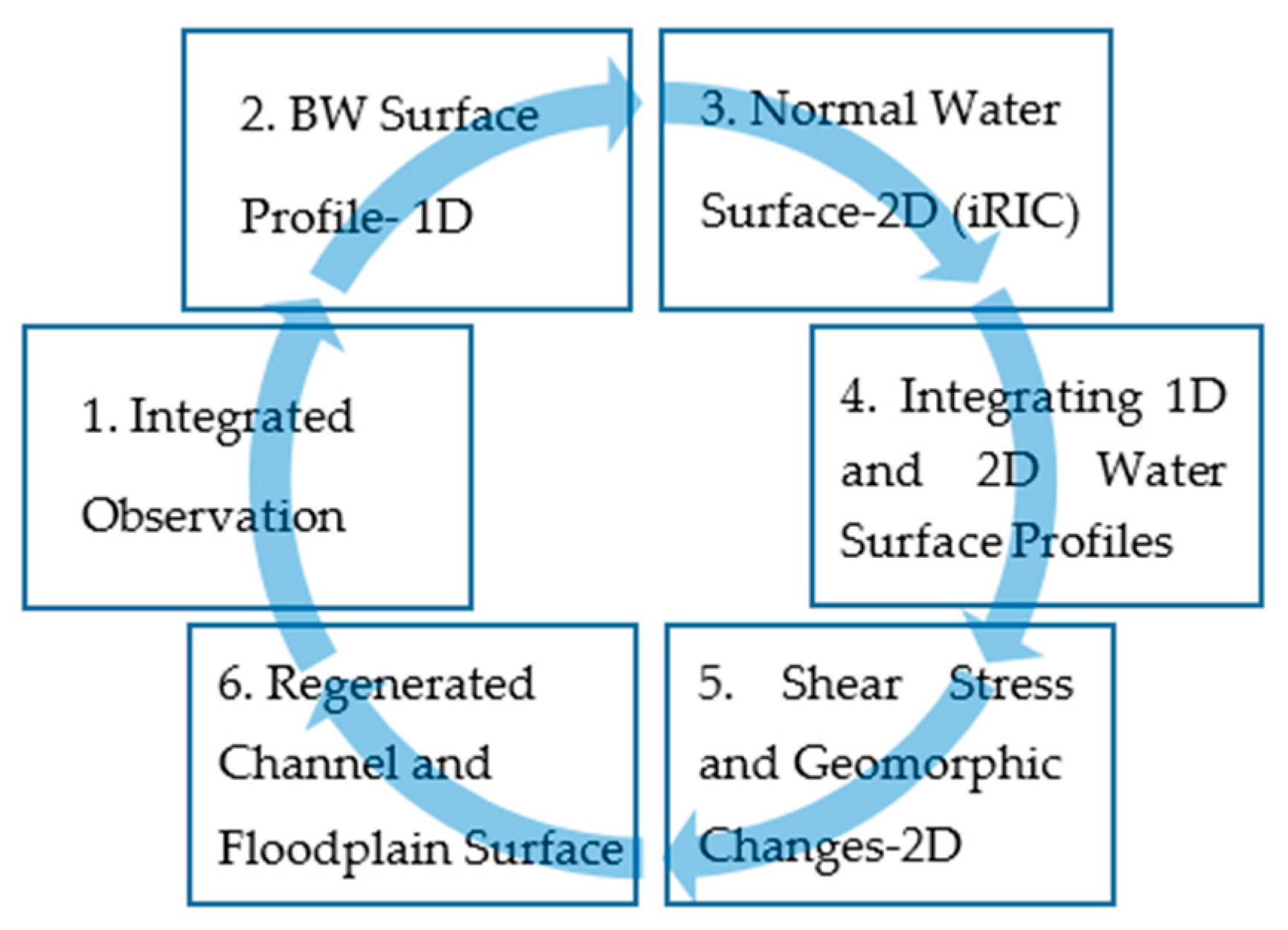
A two-dimensional shear stress model was developed to estimate the shear stress and morphological alterations in the BW and transitional zones. The output of this simulation allowed for the generating of a new digital elevation model (DEM) for the study area. The new DEM then served as a new land surface and channel bed, and the process was repeated for the next discharge. By iteratively repeating this process (Figure 2), a gradient of channel change over time was estimated.
In this paper, the 1D model refers to the model used to generate the water surface profile in the BW zone, using a modified version of Parker’s 1D model [43]. The 2D model refers to the iRIC used to estimate the 2D water surface profile and shear stress in the normal zone. The integrated model refers to the model developed to integrate and adjust water surface profiles for the whole domain based on the water surface profiles obtained from 1D and 2D models.
2.3. Data Integration
Calibrating, running, and analyzing the model required a comprehensive dataset capable of describing the geomorphic setting of the study area. The data used for this study was collected from a range of open disparate sources and integrated in a single geodatabase (Table 1).
Collecting LiDAR data for the study area is extremely difficult since it requires shutdown of the Philadelphia airport. As a result, the current DEM and bathymetric data are the most recent available data sets for the study area. In the absence of more recent data, the LiDAR based DEM and bathymetry data were merged to generate the floodplain and bathymetry of the study area.
Water surface elevation and the discharge data were obtained from the USGS gage at Cobbs Creek at Mt. Moriah Cemetery, Philadelphia (USGS gage 01475548). The hydrograph was constructed from fifteen-minute discharge data. The stage data for downstream was obtained from NOAA gages of the Delaware River (8540433, and 8545240, recorded at NAVD88 vertical datum).
Geologically, the study area is composed of primarily alluvial deposits with some sandstones, mudstones, and mica schist [51]. The banks and surface sediment are mainly silty sand [52]. At 2 rkm, three sediment samples were collected, which included one from the bed, one from the point bar and one from the bed substrate. At 4 rkm, two samples were collected which included one from the bed and one from the bank. At the time of sampling (9 November 2017), the discharge was 0.1 cubic meters per second (cms), which was the 5th percentile discharge based on recorded data. A sieving analysis was carried out to obtain the bed sediment size distribution in the creek. The grain size distribution for the upper part of the domain (2 rkm) and lower part of the domain (4 rkm) are depicted in Figure 3.
Based on the sediment samples and sieving results, the grain sizes associated with the substrate downstream with D50 = 0.0016 m and D90 = 0.0027 m were considered for further morphological analysis.
2.4. Water Surface Profile Generation
The domain of the model consists of three parts: the upper part (normal flow), the lower part (gradually varied flow or BW zone), and the transition between (Figure 1). The WSE in the upper part of the domain was modeled using the Flow and Sediment Transport with Morphological Evolution of Channels (FaSTMECH), a quasi-steady solver within the iRIC [53], while in the lower portion it was calculated using the 1D BW profile.
The 1D BW profile was developed using the 1D BW model developed by Parker [43]. Using this process, the water surface profile was generated regressively from the known water surface elevation at the mouth of the Delaware River (boundary condition) to upstream Darby Creek. The segment of the river influenced by the BW effects is a function of the mouth depth and river bed average slope expressed by:
where Lb is the BW length along the stream, H is the water depth at the mouth, and S is the average channel slope [28]. This scalar is used to differentiate between the normal and BW flow regions.
The water surface profile in BW conditions is considered to be a result of a uniform, gradually varied flow and is formulated as:
In which H is the water depth, is the bed slope, is the frictional slope, and is the Froude number [54]. In Equation (2), the sediment characteristics, such as the sediment size, affect and alter the frictional loss and consequently the frictional slope. Unlike the quasi-normal flow, the frictional slope is not relatively parallel to the bed surface and is defined as:
where is the non-dimensional bed friction coefficient. The Manning-Strickler formula defined as:
which can be used to relate the bed friction to the frictional slope, where is a constant, and is the bed roughness parameter [43]. Using Equation (2), paired with the field collected grain size data, the water surface profile for the BW zone was estimated in thalwegs in cross sections which were 5 m apart along the creek.
The iRIC output (in grid format) was analyzed in Matlab [55]. The input to the 1D BW model includes the river discharge, average river width, sediment size, and bed average slope. The 1D BW profile model was applied to the thalweg nodes along the river that were located in the BW zone. The estimated water surface elevations for the BW zone then were replaced with the iRIC values.
The start of the transitional zone has been defined as the place where the bed elevation in the creek reaches the water surface elevation at the mouth [56]. The estimated WSE from the 1D model and 2D iRIC indicated an abrupt change in the water surface elevation on either side of the transition zone. The interpolation between the two outputs was used to create a smooth transitional zone profile between the quasi-normal flow to the BW flow conditions.
The calculated water surface profile in the integrated model is the base element in deriving the shear stress and eventually, the morphological alterations in the BW and transitional zones, but it is difficult to verify. The LiDAR data collected on 25 April, 2015 was used to determine the measured water surface elevation along the creek. The USGS Cobbs Creek gage records in the upstream showed that the discharge associated with that date was 0.42 cms which is considered as a moderate flow (flow between 20th and 80th percentiles of the discharges [57,58]) in Darby Creek. For this analysis, the water surface elevation points were obtained from the locations in the creek close to the banks rather than near the middle. This methodology minimized drastic WSE changes. The integrated model was then run for a discharge of 0.42 cms to obtain the estimated water surface elevation. Figure 4 shows the comparison between the estimated and measured water surface profiles. Choosing points from LiDAR data to obtain water surface profiles can be arbitrary because of the cloud point format of the high-resolution elevation data. The elevation differences in adjacent points over the water surface—which may vary approximately up to 10 percent—can be related to the lateral variations in the water surface elevation across the river, remote sensing errors and noises, the presence of different suspended materials and waves on the surface of the flow.
The adjusted water surface profile was then used to estimate the water depth in the BW and transitional zones. By assuming that the water surface elevation was constant across the cross section, the depth at each node in the cross section was calculated as:
where h is the water depth, WSE is the water surface elevation estimated from the 1D BW model, and Z is the land surface elevation.
2.5. Hydraulic Model Analysis
The described model uses an integral approach to simulate (a) the hydraulics of the flow in BW and quasi-normal zones and (b) the morphological alterations in the quasi-normal zone as well as the BW zone. The calibration of the 2D iRIC model was carried out by setting up the model so that it matched with the water surface elevation registered in the USGS Cobbs Creek gage for a specific discharge. The selected event for the model calibration occurred on 30 August, 2009 and registered a peak water surface elevation of 12 m with the maximum discharge of 184 cms. A 72-h observed hydrograph for this event was used along with the frictional coefficients within the iRIC to match the water surface elevation with the observed value. The methodology used was similar to the methodology from Zarzar et al. [39].
2.6. Modeling Flood Extent, Frictional Slope, and Shear Stress
The two regions of normal and gradually varied flow were differentiated. The 1D BW profile provided water surface elevation in the BW zone, which was used to generate 2D depth values. Coupling the 2D iRIC model with the 1D BW model resulted in an integrated model that was capable of addressing morphological alterations in the presence of BW. For the upper domain, where the flow is quasi-normal, 2D shear stresses () calculated by iRIC were considered to estimate sediment discharge. However, for the lower domain, a new model had to be developed to account for the BW hydraulics.
The total bed shear stress for both the uniform and non-uniform flow can be estimated by:
where is the mean longitudinal shear stress applied on the perimeter of the channel, is the hydraulic radius, and Sf is the slope of the total energy line or frictional slope [59]. In the uniform flow, the frictional slope is equal to the bed slope, while in the gradually varied flow, they are not equal.
The frictional slope is nonlinearly related to discharge and the conveyance factor (K) as:
In which K is defined as,
where A is the area of the flow, and n is the Manning coefficient [12]. The conveyance factor is a function of the flow depth. Therefore, if the depth is known, the frictional slope can be calculated.
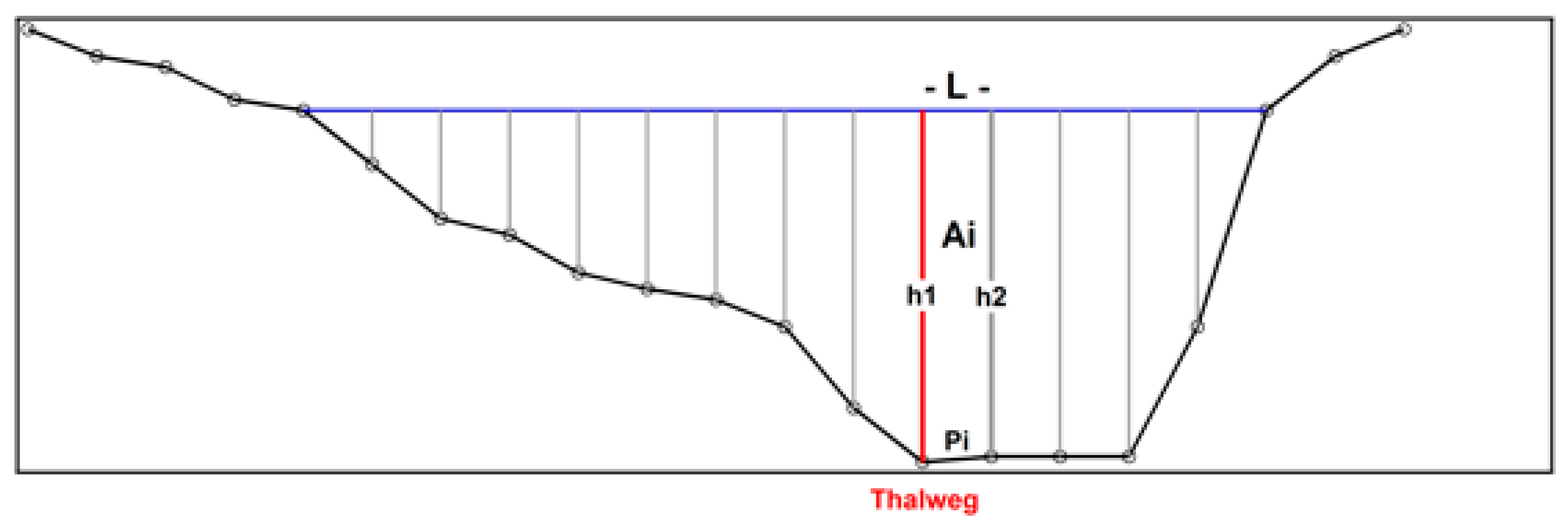
To calculate the shear stress in the BW zone across the cross section, each cross section in the BW zone was divided into segments perpendicular to the flow so that each node separated two adjacent segments (Figure 5).
To calculate the depth in the BW zone, the 1D morphodynamic model developed by Parker [43] was adopted to estimate the water surface profile along the thalweg of the river (h1 in Figure 5). In this way, the water surface elevation over the thalweg at each cross section was estimated. By assuming that WSE does not change substantially across the cross sections in the BW zone, the depth of the water at any point in each cross section could be estimated as the difference between WSE and natural ground elevation.
The wetted perimeter for each segment () was the part of the bed confined between two nodes. By having a large number of nodes in each cross section, the distances between nodes was relatively small and therefore, the wetted perimeter for each segment was calculated as:
The hydraulic radius for each segment () was calculated for each segment as:
The conveyance factor then was calculated for each segment as:
The discharge associated with each segment (Qi) was estimated by assuming that the discharge in each segment was linearly related to the area of the segment relative to the area of the whole cross section as:
The frictional slope for each segment in a cross section can be estimated based on Equation (3) as:
Once the frictional slope was obtained, using Equation (6), the shear stress (τ) associated with each node and Shields parameter () was calculated as:
where and are the sediment and water density, g is gravity, and is the characteristic sediment size, which indicates a sediment size smaller than 50 percent of the bed grains. The calculated shear stresses and sediment transport across each cross section are longitudinal and in the direction of the stream. To reduce the complexity, it was assumed that the shear stress in the y direction is negligible in the BW zone.
2.7. Geomorphic Analysis
The output of the iRIC, including the generated mesh and associated coordinates, depth of flow, ground elevation, flood extent, velocity, and shear stress fields, was imported into Matlab [55] to address the BW conditions and bed elevation change. This procedure was followed to model sediment transport and morphological changes in all nodes in each cross section (Figure 5) of the domain.
Once the shear stress domain in the BW zone was identified, the Meyer-Peter and Müller (MPM) Equation [60] was used to estimate the sediment discharge in both the BW and quasi-normal regions. The MPM, one of the most widely used equations in geomorphology [61], is used to estimate the bedload in mountain streams with gravel and coarse sand. However, it has also been widely used in coastal sediment transport [62]. The MPM sediment bedload discharge is based on the available excess non-dimensional shear stress as:
where and are the sediment transport coefficients, is the non-dimensional shear stress applied on the bed, is the non-dimensional shear stress associated with incipient motion equal to 0.047, and is non-dimensional volume shear stress rate per unit width. The is defined as:
where is the volumetric bedload discharge per unit width.
The original value of α and β in MPM is 8 and 1.5 for gravel. However, the α value was adjusted from 8 to 12 to make the equation applicable for sand by implying a higher sediment transport rate [63,64]. The estimated bedload discharge was used in conjunction with the 2D Exner Equation to characterize bed elevation change as:
where is the bed sediment porosity, is the bed elevation, t is the simulation time step, and and are sediment discharge in the x and y directions. This calculation gives the bed elevation changes over the quasi-normal and BW regions. However, at the transition between the quasi-normal and BW zones, a diffuser function, similar to the one suggested by Liang et al. [65] was applied to smooth this transition. The adjustment was applied to nodes in the vicinity of the flow transition. The diffuser uses the averaged bed elevation changes of the neighboring nodes as:
where ε is the diffusivity coefficient, and n is the number of the neighboring nodes used in the calculations. ε = 0.1 and n = 2 were used in the calculations based on iterative trials, and the results were checked to ensure that the smooth bed elevation changes took place in the flow transition zone. To aid in obtaining stable solutions, an under relaxation scheme was applied to ensure numerical stability [65] as:
where the under-relaxation coefficient, ω, was set to 0.1. The new bed elevation, was used to update the DEM in each time step of the simulation with the results of the changes in sediment discharge.
2.8. Iterative Process
The new DEM was used to rerun the integrated model in an iterative fashion. The hydraulic models were run again to simulate the hydraulics of the flow for the next discrete discharge. The calculations continued reciprocally for the discrete discharges, representing flood events of the hydrograph. The peak discharges in the hydrograph that were above the incipient discharge (the discharge that sediment movement initiates) were considered for the simulations. Once a set of discrete discharges was obtained, the integrated model was run for each discharge to obtain the elevation change in bathymetry and banks due to that particular discharge. The updated DEM was then used for the next discharge simulation. The iterative process can be automated using the Matlab as the platform which enhances the computational efficiency, specifically for long simulations.
2.9. Verification of Geomorphic Model
The verification of any geomorphological model requires both the floodplain and bathymetry elevation data before and after specific events. Due to a lack of such data for Darby Creek, satellite images provided insight into morphological alterations in the study area. Landsat satellite images have been widely used by researchers as a benchmark for ground proof data [66,67] regarding morphological alterations. The changes in land surface by erosion (or deposition) eventually result in a change in surface spectral reflectance [68].
In addition to image classification methods, surface spectral reflectance can be used for erosion (and deposition) mapping [68]. This method was applicable to the lower part of the Darby Creek, where the creek bed broadens and forms a wide marsh area along with exposed bars in low discharges. Unlike the upper part of the creek, the lower part of the creek is not covered with trees and vegetation, and therefore land changes are more detectable by satellite images.
The higher discharges are more likely to cause significant morphological alterations in a window of a few months. In addition, using peak discharges in a cyclic manner can represent unsteady conditions over the period of the study [69]. The highest registered flood in Darby Creek was selected for verifying the morphological alterations predicted by the integrated model. According to USGS peak stream flow data (which has only been gathered since 2006), the highest registered flood happened on 8 September, 2011 with a maximum discharge of 164 cms, which was approximately twice the bankfull discharge.
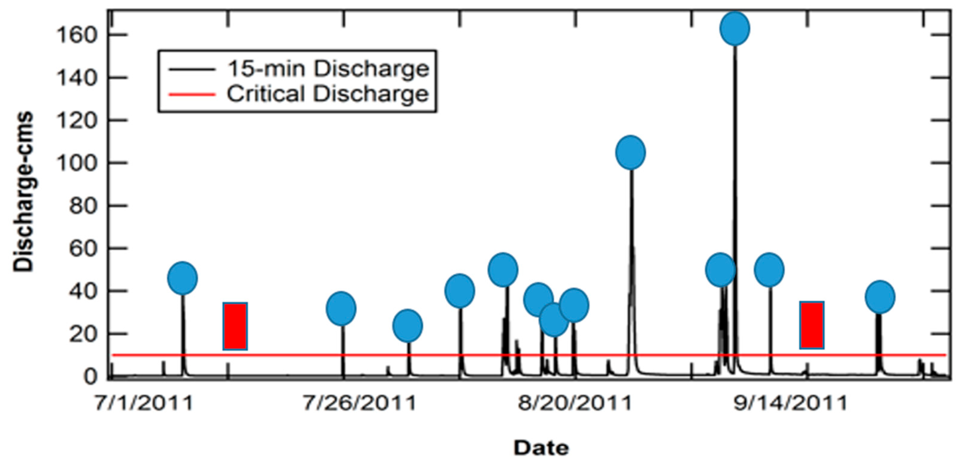
Two cloud-free Landsat images from 2011 (14 July and 16 September) were obtained from Earth Explorer Landsat Analysis Ready Data [70]. The discharge data from 14 July to 16 September 2011 revealed that there were frequent medium floods in that time window. The assumption was that significant morphological alterations are limited to large events, specifically in BW conditions [22]. In order to filter out the low discharges, the Schoklitsch Equation [71] was used to find the critical discharge as:
in which is the critical discharge per unit width at which bedload motion initiates, is the sediment size (m), and S is the bed slope. By considering S = 7.04 × 10⁻⁴, = 0.0013 m and an average width of 70 m for Darby Creek, the critical discharge was estimated and rounded up to 10 cms. Filtering out the low discharges and selecting the peak discharges resulted in serial peak discharges (shown as circles in Figure 6).
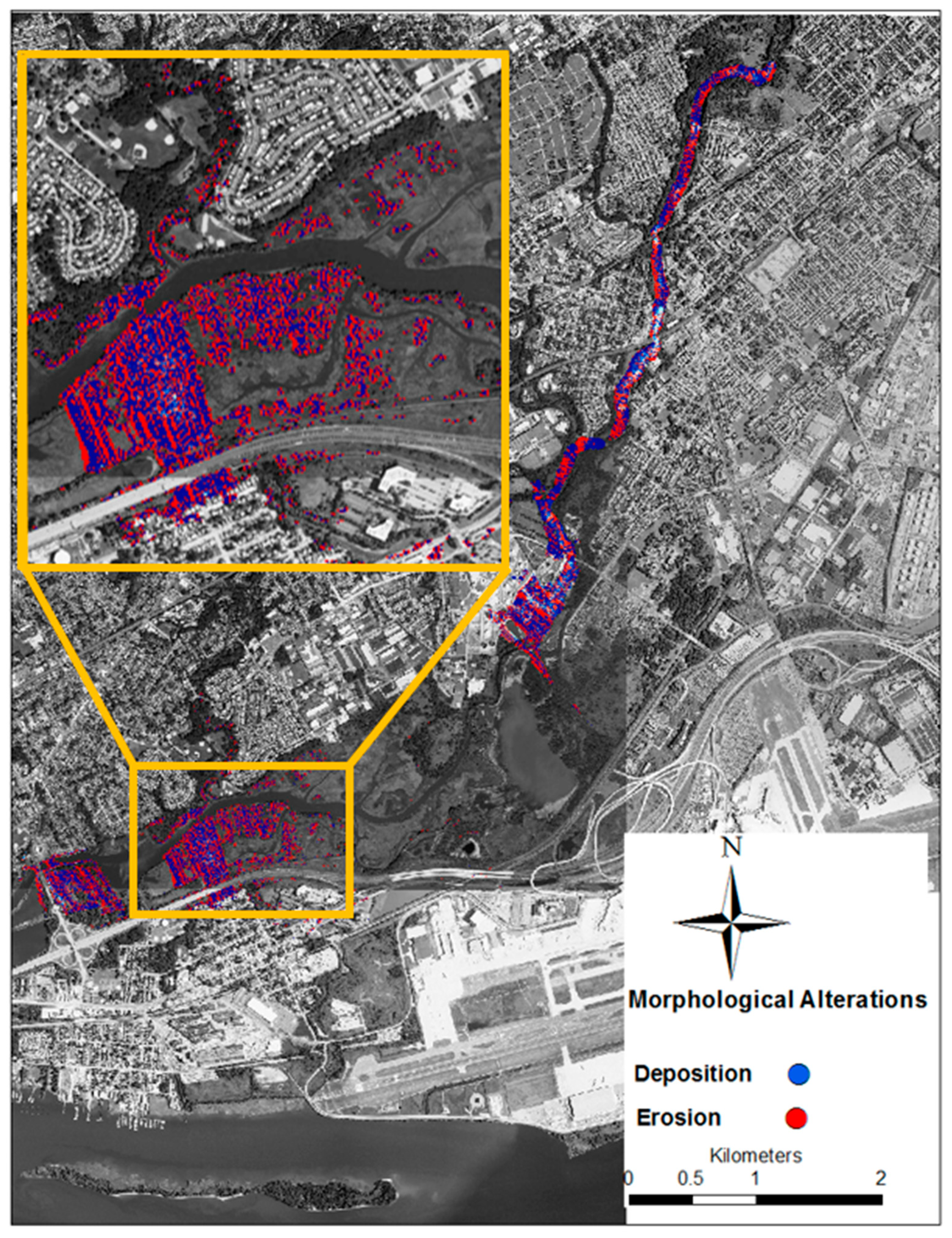
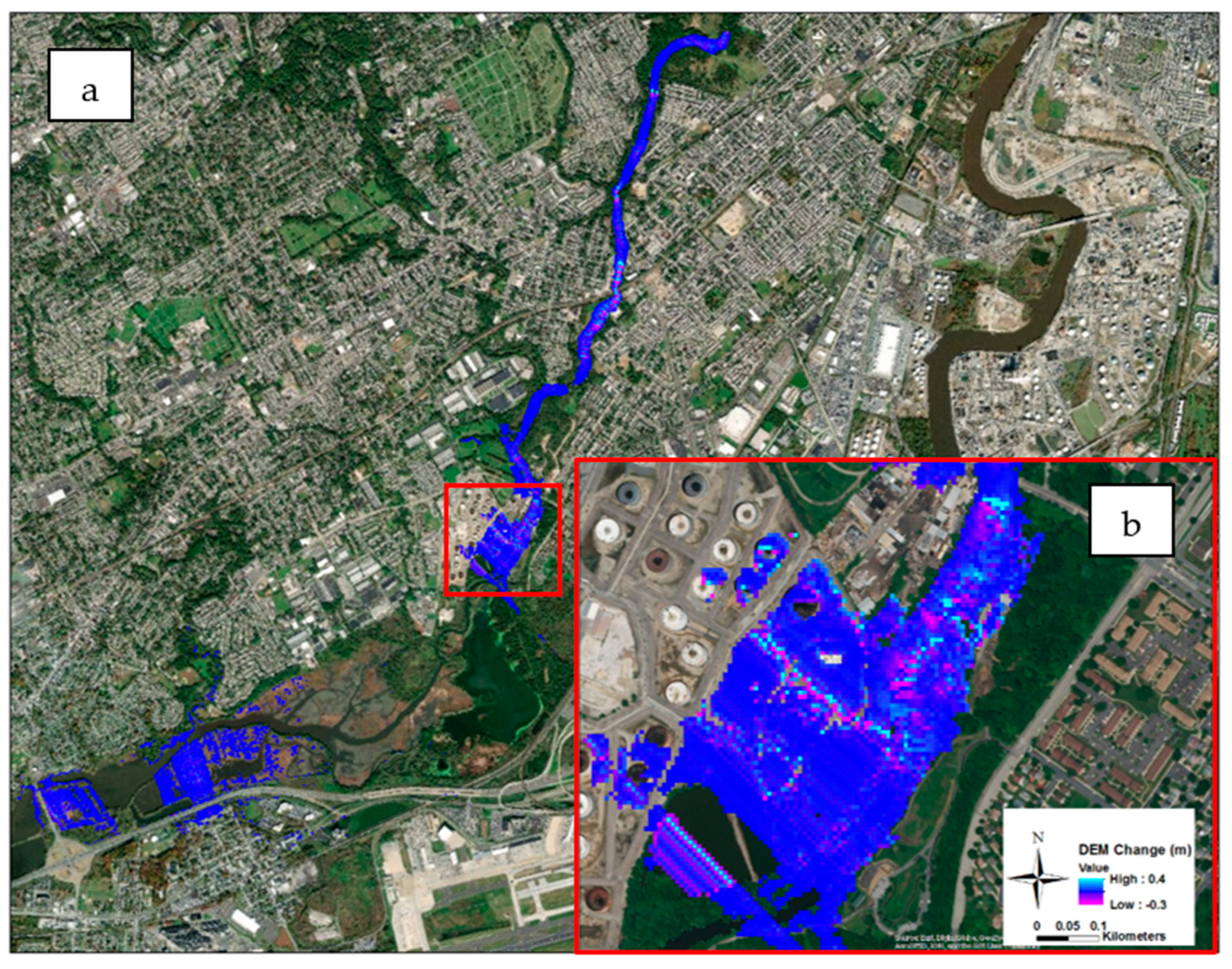
The differences in land surface spectral reflectance were mapped in ArcGIS [72]. The areas covered by water were masked out from the images to ensure that the changes in reflectance were due only to land surface changes. The normalized difference water index (NDWI) was used to differentiate between the water, vegetation and soil [73,74]. A change detection technique was required for finding the change in reflectance values in the satellite images. This was done through a raster subtraction to find the difference in reflectance values in the two images. The reflectance value in each cell associated with 16 September was subtracted from the reflectance value for 14 July. Zero values in the results indicated no morphological changes, and non-zero values indicated potential land surface disturbances and possible morphological alterations. Although this change detection analysis between the dates does not discriminate between erosion and deposition (Figure 7a), the higher the reflectance, the more likely there will be increased land surface disturbance (erosion or deposition of the sediment) resulting from a flood event [68]. The output of the integrated model can predict and discriminate where erosion and deposition will occur (Figure 7b).
3. Results and Discussion
3.1. Analysis of Water Surface Elevation
The critical depth associated with the maximum discharge in the simulations (164 cms) and the average river width of 70 m was estimated as 0.82 m, which was smaller than the normal depth estimated by the iRIC (yn > yc) over the thalweg in the BW zone. This indicates a mild slope and M water surface profile of the study area. The water surface elevation in the Delaware River varies between 0 to 2 m due to tidal conditions (Markus Hook NOAA gage). An average WSE of 1 m was used in the hydraulic models for the downstream boundary condition, which implies a depth value higher than normal (y > yn; y > yc), suggesting an M1 water surface profile. This was true for all discharges.
3.2. Analysis of the Geomorphic Model
The results of the integrated model showing areas of change generally agreed with the surface changes captured by the Landsat images. Both methods captured the reduction in the geomorphic changes in the transitional zone between the quasi-normal and the BW zones. Both methods also showed that at the end of the transitional zone where the BW zone initiates, no significant erosion or deposition occurred. Further, both approaches were congruent in regard to the morphological alterations in the marsh area in the lower part of the creek in the BW zone. This suggests active banks with frequent erosion and deposition, indicating the presence of sediment transport in the BW zone from the river to the banks and vice versa [75,76]. Unlike the model results, the satellite images indicated the occurrence of some morphological alterations in the marsh area in the middle of BW zone (Figure 7).
The satellite images captured more morphologic activity in the marsh relative to the model prediction. The slight differences in the lower part of the domain might be related to the following issues:
- (a)
- The presence of water over the land, and that the ground information had not been captured by the satellite images.
- (b)
- A single discharge simulation rather than a full hydrograph did not capture the differences. That means that with regard to morphological alterations, a single discharge might poorly represent a hydrograph.
- (c)
- The vegetation present when the satellite images were captured could cause differences.
- (d)
- The discrepancy between the model and the satellite images also might stem from sensitivity of the model toward the selected sediment size, because it is based on a single grain size. A sensitivity analysis was conducted to test the model’s sensitivity to sediment grain size.
- (e)
- The choice of the sediment transport equation used in the model. The integrated model can be enhanced by including other transport models that can address the mobility of different sediment sizes.
The purpose of validating the integrated model by using Landsat images was not to compare it with the model output in quantifiable terms, but was to merely provide some insight into land evolution in BW conditions and to ensure that the model depicted what was happening in nature. The model predicts where erosion or deposition occurs on a relative scale, rather than predicting the quantity of the moved or deposited sediment. The output of the model includes the adjusted water surface elevation for the BW and the transitional zones, and the spatial distribution of erosion and deposition. Recently measured elevation data is required to enhance the verification, validation, and justification of the model. However, in the absence of those data, the proposed validation method suggested above provides an insight into the possible morphological alterations in lower Darby Creek. More specifically, the Landsat images suggest a substantial reduction in erosion and deposition of sediment in transitioning from normal to a gradually varied flow which was captured by model. This is in agreement with the results from Lu et al. [18], where they showed an increase in the cross sectional area in the BW zone decreases the flow velocity and sediment transport capacity. In addition, the satellite images showed evidence of erosion and deposition of sediment in the lower part of the creek over the marsh area, which was captured by the model too. The model results showed that the banks in the BW zone in Darby Creek are actively experiencing drowning which results in active erosion and deposition of sediment on the banks. (Figure 8).This is in agreement with the findings of Maselli et al. [11] and Liro [9].
In the upstream area (normal zone in Figure 1), the presence of the trees and bushes along the creek might bias the Landsat change results [77]. However, for the lower part in the BW zone that issue is less significant, as the vegetation is less dense. Once the rates of erosion and deposition were identified for all nodes within the domain, by integrating all erosion and deposition for each node, a raster of morphologic alterations for the whole domain was obtained (Figure 9).
As expected, the model output showed that higher discharges caused more geomorphic alterations. Comparing the geomorphic alteration simulated by the model for both BW and quasi-normal zones suggested that the geomorphological changes in the BW zone were more sensitive to changes in the discharge. This indicated that the critical discharge in the BW conditions was higher than the one in the quasi-normal flow. For discharges lower than 42 cms, no morphological alterations took place in the BW zone, and in the quasi-normal zone, the morphological alterations below 22 cms were negligible. The developed geomorphic model was based on a single grain size, which may result in an uncertainty in the predicted geomorphic alterations. The sensitivity analysis of the integrated model relative to the grain size (D50) showed that the geomorphic activities in both the quasi-normal and BW zones decreased with an increase in sediment size, which was expected. However, the BW zone was more sensitive to changes in the sediment size. The model predicted almost no geomorphic changes in the BW zone for any grain size larger than 6 and in the normal zone, no geomorphic changes for grain sizes larger than 35 mm.
4. Conclusions
BW conditions occur in rivers mainly within the coastal zone, near the confluence of the river and sea, and in upstream of dam reservoirs which is where the majority of the world’s population lives. Understanding the fluvial morphodynamics of these hydraulic conditions could substantially contribute to flood mitigation, river restoration, and environmental protection. The complex hydraulics along with a lack of measured data make the critical issue of understanding and predicting fluvial morphodynamics in BW zones increasingly challenging. In addition, there are no 2D morphological models for the BW and transitional zones. This work presents an integrated 2D model that contributes to the efforts to enhance our understanding of geomorphological alterations in these zones. The intention of this paper is to initially develop the integrated model in a simple form to show a representative change or gradient of change. This model does not attempt to truly quantify the degree of change, just the areas of change. The model aims to enhance our understanding of morphodynamics in BW zones by addressing spatial erosion or deposition over the domain. To do this, an integrative approach was defined to integrate and adjust the water surface profiles in the BW, normal and transitional zones. The adjusted water surface profile derived calculations of shear stresses in each cross section in the BW and transitional zones. The erosion, deposition, and consequently bed elevation changes were estimated based on the calculated sediment transport discharges. Through an iterative process, this study was able to consider a quasi-continuous hydrograph run. The integrated model generated a new DEM of the study area, which served as the starting point for the next iteration of flow, ultimately modeling geomorphic changes through time. The model output included an integrated water surface profile, an adjusted 2D shear stress domain, a morphological alteration map segregating erosion and deposition, the total amount of the rate of erosion and deposition, the DEM change, and an updated DEM. For model validation and verification, the model was applied to Darby Creek in the Metro-Philadelphia area of Pennsylvania. The model was run for this study area using a range of discharges for the simulation time of one hour. The simulated water surface profile and morphological alteration map were tested against LiDAR surveys and Landsat images, respectively. Landsat images spanning three months suggested a strong spatial correlation between the model results and the presence of geomorphic change. The simulation results for the different discharges in Darby Creek show that the critical discharge (the discharge at which morphological activities start to happen) for the BW zone is higher than the one for the quasi-normal flow. This implies no significant morphological changes in the BW zones in the low flows until the discharges rose to a certain threshold. The model results show that the banks in the BW zone in Darby Creek are actively experiencing erosion and deposition of the sediment. This implies an active reciprocal sediment transport from the creek to the banks and vice versa. In addition, the model showed a reduction in morphological alterations at transitioning zone from normal to a gradually varied flow. These findings shed light on the potential impact of major storms on stream morphology in the BW zones and how the floodplain will potentially change over time. The integrated model, along with proposed framework, can simulate continuous morphological changes in BW conditions for an intermediate time scale (over decades) which can serves as an important tool in guiding the land and resource management efforts, planning for sustainable infrastructure, and mitigating the impacts of climate change.
Author Contributions
Conceptualization, H.H. and V.S.; methodology, H.H. and V.S.; Writing—Original Draft preparation, H.H.; Writing—Review and Editing, V.S. and H.H.; visualization, H.H.; supervision, V.S.; project administration, V.S.; funding acquisition, V.S.
Funding
This research was funded by Civil and Environmental Engineering Department of Villanova University.
Acknowledgments
The idea for this research began with the Summer Institute Innovator Program in 2016, held by the National Water Center in Alabama in a joint work with the Consortium of Universities for the Advancement of Hydrologic Science (CUAHSI). We would like to thank all the staff who organized the program, with special thanks to David Maidment and Edward Clark. We appreciate all the colleagues and students in Villanova Center for Resilience Water Systems (VCRWS) for their help, support, and feedback throughout the development of this project. Also we would like to thank the John Heinz Wildlife Refuge management and staff for their cooperation with data collection. Specifically, we would like to thank Brendalee Philips for sharing her knowledge on Darby Creek with us and supporting this project. Finally, we would like to thank Ward Barnes for sharing his insight with us during the creation of this manuscript. The data used in this study can be accessed from online sources (Table 1) listed in the reference section.
Conflicts of Interest
The authors declare no conflict of interest. The funders had no role in the design of the study; in the collection, analyses, or interpretation of data; in the writing of the manuscript, or in the decision to publish the results.
References
- National Oceanic and Atmospheric Administration. Land-Based Station Data | National Centers for Environmental Information (NCEI) Formerly Known as National Climatic Data Center (NCDC). Available online: https://www.ncdc.noaa.gov/data-access/land-based-station-data/land-based-datasets (accessed on 10 May 2019).
- Census Urban and Rural Classification and Urban Area Criteria. 2010. Available online: https://www.census.gov/geo/reference/ua/urban-rural-2010.html (accessed on 26 March 2019).
- Creel, L. Ripple Effects: Population and Costal Regions; Population Reference Bureau, Making the Link: Washington, DC, USA, 2003; pp. 1–8. [Google Scholar]
- Kummu, M.; De Moel, H.; Salvucci, G.; Viviroli, D.; Ward, P.J.; Varis, O. Over the Hills and Further Away from Coast: Global Geospatial Patterns of Human and Environment over the 20th–21st Centuries. Environ. Res. Lett. 2016, 11, 034010. [Google Scholar] [CrossRef]
- Neumann, B.; Vafeidis, A.T.; Zimmermann, J.; Nicholls, R.J. Future Coastal Population Growth and Exposure to Sea-Level Rise and Coastal Flooding—A Global Assessment. PLoS ONE 2015, 10, e0118571. [Google Scholar] [CrossRef] [PubMed]
- Desmet, K.; Kopp, R.E.; Kulp, S.A.; Nagy, D.K.; Oppenheimer, M.; Rossi-hansberg, E.; Strauss, B.H. Evaluating the Economic Cost of Coastal Flooding; National Bureau of Economic Research Working paper No. 24918; National Bureau of Economic: Cambridge, MA, USA, 2018. [Google Scholar]
- Yang, Y.; Zhang, M.; Zhu, L.; Liu, W.; Han, J.; Yang, Y. Influence of Large Reservoir Operation on Water-Levels and Flows in Reaches below Dam: Case Study of the Three Gorges Reservoir. Sci. Rep. 2017, 7, 1–14. [Google Scholar] [CrossRef] [PubMed]
- Volke, M.A.; Johnson, W.C.; Dixon, M.D.; Scott, M.L. Emerging Reservoir Delta-Backwaters: Biophysical Dynamics and Riparian Biodiversity. Ecol. Monogr. 2019, 89, 1–22. [Google Scholar] [CrossRef]
- Liro, M. Dam Reservoir Backwater as a Field-Scale Laboratory of Human-Induced Changes in River Biogeomorphology: A Review Focused on Gravel-Bed Rivers. Sci. Total Environ. 2019, 651, 2899–2912. [Google Scholar] [CrossRef] [PubMed]
- Fencl, J.S.; Mather, M.E.; Costigan, K.H.; Daniels, M.D. How Big of an Effect Do Small Dams Have? Using Geomorphological Footprints to Quantify Spatial Impact of Low-Head Dams and Identify Patterns of across-Dam Variation. PLoS ONE 2015, 10, 1–22. [Google Scholar] [CrossRef]
- Maselli, V.; Pellegrini, C.; Del Bianco, F.; Mercorella, A.; Nones, M.; Crose, L.; Guerrero, M.; Nittrouer, J.A. River Morphodynamic Evolution Under Dam-Induced Backwater: An Example from the Po River (Italy). J. Sediment. Res. 2018, 88, 1190–1204. [Google Scholar] [CrossRef]
- Chow, V.T. Open-Channel Hydraulics. In Ven Te Chow; McGraw-Hill: New York, NY, USA, 1959. [Google Scholar]
- Dingman, S.L. Fluvial Hydrology; W.H. Freeman and Company: New York, NY, USA, 1984. [Google Scholar]
- Jin, Z.W.; Lu, J.Y.; Wu, H.L. Study of Bedload Transport in Backwater Flow. J. Hydrodyn. 2016, 28, 153–161. [Google Scholar] [CrossRef]
- Xu, J. Evolution of Mid-Channel Bars in a Braided River and Complex Response to Reservoir Construction: An Example from the Middle Hanjiang River, China. Earth Surf. Process. Landf. 1997, 22, 953–965. [Google Scholar] [CrossRef]
- Xu, J. Modified Conceptual Model for Predicting the Tendency of Alluvial Channel Adjustment Induced by Human Activities. Chin. Sci. Bull. 2001, 46, 51–56. [Google Scholar] [CrossRef]
- Munier, S.; Litrico, X.; Belaud, G.; Malaterre, P.O. Distributed Approximation of Open-Channel Flow Routing Accounting for Backwater Effects. Adv. Water Resour. 2008, 31, 1590–1602. [Google Scholar] [CrossRef]
- LU, Y.; ZUO, L.; JI, R.; LIU, H. Deposition and Erosion in the Fluctuating Backwater Reach of the Three Gorges Project after Upstream Reservoir Adjustment. Int. J. Sediment Res. 2010, 25, 64–80. [Google Scholar] [CrossRef]
- Hidayat, H.; Vermeulen, B.; Sassi, M.G.; Torfs, P.J.J.F.; Hoitink, A.J.F. Discharge Estimation in a Backwater Affected Meandering River. Hydrol. Earth Syst. Sci. 2011, 15, 2717–2728. [Google Scholar] [CrossRef]
- Liro, M. Development of Sediment Slug Upstream from the Czorsztyn Reservoir (Southern Poland) and Its Interaction with River Morphology. Geomorphology 2016, 253, 225–238. [Google Scholar] [CrossRef]
- Liro, M. Dam-Induced Base-Level Rise Effects on the Gravel-Bed Channel Planform. Catena 2017, 153, 143–156. [Google Scholar] [CrossRef]
- Nittrouer, J.A.; Shaw, J.; Lamb, M.P.; Mohrig, D. Spatial and Temporal Trends for Water-Flow Velocity and Bed-Material Sediment Transport in the Lower Mississippi River. Bull. Geol. Soc. Am. 2012, 124, 400–414. [Google Scholar] [CrossRef]
- Chow, V.T. Open Channel Hydraulics; The Blackburn Press: Caldwell, NJ, USA, 1959. [Google Scholar]
- Chatanantavet, P.; Lamb, M.P.; Nittrouer, J.A. Backwater Controls of Avulsion Location on Deltas. Geophys. Res. Lett. 2012, 39, 2–7. [Google Scholar] [CrossRef]
- Fernandes, A.M.; Törnqvist, T.E.; Straub, K.M.; Mohrig, D. Connecting the Backwater Hydraulics of Coastal Rivers to Fluviodeltaic Sedimentology and Stratigraphy. Geology 2016, 44, 979–982. [Google Scholar] [CrossRef]
- Lamb, M.P.; Nittrouer, J.A.; Mohrig, D.; Shaw, J. Backwater and River Plume Controls on Scour Upstream of River Mouths: Implications for Fluvio-Deltaic Morphodynamics. J. Geophys. Res. Earth Surf. 2012, 117, 1–16. [Google Scholar] [CrossRef]
- Zhang, X.; Jin, D.; Lu, X.H. Friction Velocity in Decelerating Open Channel Flow. Huazhong Univ. Sci. Technol. 2014, 42, 113–118. [Google Scholar]
- Mohrig, D.; Paola, C. Palaeohydraulics Revisited: Palaeoscope Estimation in Coarse Grained Braided Rivers. Basin Res. 1996, 8, 243–254. [Google Scholar]
- Trower, E.J.; Ganti, V.; Fischer, W.W.; Lamb, M.P. Erosional Surfaces in the Upper Cretaceous Castlegate Sandstone (Utah, USA): Sequence Boundaries or Autogenic Scour from Backwater Hydrodynamics? Geology 2018, 46, 707–710. [Google Scholar] [CrossRef]
- Durkin, P.R.; Boyd, R.L.; Hubbard, S.M.; Shultz, A.W.; Blum, M.D. Three-Dimensional Reconstruction of Meander-Belt Evolution, Cretaceous Mcmurray Formation, Alberta Foreland Basin, Canada. J. Sediment. Res. 2017, 87, 1075–1099. [Google Scholar] [CrossRef]
- Ganti, V.; Lamb, M.P.; Chadwick, A.J. Autogenic Erosional Surfaces in Fluvio-Deltaic Stratigraphy from Floods, Avulsions, and Backwater Hydrodynamics. J. Sediment. Res. 2019, 89, 815–832. [Google Scholar] [CrossRef]
- Chadwick, A.J.; Lamb, M.P.; Moodie, A.J.; Parker, G.; Nittrouer, J.A. Origin of a Preferential Avulsion Node on Lowland River Deltas. Geophys. Res. Lett. 2019, 46, 4267–4277. [Google Scholar] [CrossRef] [Green Version]
- Ganti, V.; Chadwick, A.J.; Hassenruck-Gudipati, H.J.; Fuller, B.M.; Lamb, M.P. Experimental River Delta Size Set by Multiple Floods and Backwater Hydrodynamics. Sci. Adv. 2016, 2, 1–11. [Google Scholar] [CrossRef]
- Blum, M.; Martin, J.; Milliken, K.; Garvin, M. Paleovalley Systems: Insights from Quaternary Analogs and Experiments. Earth Sci. Rev. 2013, 116, 128–169. [Google Scholar] [CrossRef]
- Colombera, L.; Mountney, N.P.; Russell, C.E.; Shiers, M.N.; McCaffrey, W.D. Geometry and Compartmentalization of Fluvial Meander-Belt Reservoirs at the Bar-Form Scale: Quantitative Insight from Outcrop, Modern and Subsurface Analogues. Mar. Pet. Geol. 2017, 82, 35–55. [Google Scholar] [CrossRef]
- Ganti, V.; Chu, Z.; Lamb, M.P.; Nittrouer, J.A.; Parker, G. Testing Morphodynamic Controls on the Location and Frequency of River Avulsions on Fans versus Deltas: Huanghe (Yellow River), China. Geophys. Res. Lett. 2014, 41, 7882–7890. [Google Scholar] [CrossRef]
- Shiers, M.N.; Mountney, N.P.; Hodgson, D.M.; Colombera, L. Controls on the Depositional Architecture of Fluvial Point-Bar Elements in a Coastal-Plain Succession, 1st ed.; Ghinassi, M., Colombera, L., Mountney, N.P., Reesink, A.J.H., Eds.; John Wiley & Sons Ltd.: Cambridge, UK, 2018. [Google Scholar] [CrossRef]
- Martin, J.; Fernandes, A.M.; Pickering, J.; Howes, N.; Mann, S.; Mcneil, K. The Stratigraphically Preserved Signature of Persistent Backwater Dynamics in a Large Paleodelta System: The Mungaroo Formation, North West Shelf, Australia. J. Sediment. Res. 2018, 88, 850–872. [Google Scholar] [CrossRef]
- Zarzar, C.M.; Hosseiny, H.; Siddique, R.; Gomez, M.; Smith, V.; Mejia, A.; Dyer, J. A Hydraulic MultiModel Ensemble Framework for Visualizing Flood Inundation Uncertainty. JAWRA J. Am. Water Resour. Assoc. 2018, 54, 807–819. [Google Scholar] [CrossRef]
- Bauer, M.; Dostal, T.; Krasa, J.; Jachymova, B.; David, V.; Devaty, J.; Strouhal, L.; Rosendorf, P. Risk to Residents, Infrastructure, and Water Bodies from Flash Floods and Sediment Transport. Environ. Monit. Assess. 2019, 191, 85. [Google Scholar] [CrossRef] [PubMed]
- Philadelphia City Council Hearing Testimony on Behalf of Clean Air Council, Clean Water Action. Available online: https://www.pubintlaw.org/wp-content/uploads/2012/06/Environmental-Groups-Testimony.pdf (accessed on 10 May 2019).
- National Wildlife Refuge System. John Heinz National Wildlife Refuge at Tinicum Habitat Management Plan July 2009; U.S. Fish and Wildlife Service: Philadelphia, PA, USA, 2009.
- Parker, G. 1D Sediment Transport Morphodynamics with Applications to Rivers and Turbidity Currents: E-Book; St. Anthony Falls Laboratory, University of Minnesota: Minneapolis, MN, USA, 2004. [Google Scholar]
- Pennsylvania Spatial Data Access Data Summary. Available online: http://www.pasda.psu.edu/uci/DataSummary.aspx?dataset=1248 (accessed on 12 October 2018).
- Pennsylvania Spatial Data Access Data Summary. Available online: http://www.pasda.psu.edu/uci/DataSummary.aspx?dataset=1048 (accessed on 12 October 2018).
- Bathymetric Data Viewer. Available online: https://maps.ngdc.noaa.gov/viewers/bathymetry/ (accessed on 12 October 2018).
- USGS Current Conditions for USGS 01475548 Cobbs Creek at Mt. Moriah Cemetery, Philadelphia. Available online: https://nwis.waterdata.usgs.gov/pa/nwis/uv/?cb_00065=on&cb_00060=on&format=gif_default&site_no=01475548&period=&begin_date=2014-04-29&end_date=2014-04-30 (accessed on 12 October 2018).
- Marcus Hook, PA—NOAA Tides and Currents 8540433. Available online: https://tidesandcurrents.noaa.gov/ports/ports.html?id=8540433 (accessed on 10 May 2019).
- Philadelphia, PA—NOAA Tides and Currents 8545240. Available online: https://tidesandcurrents.noaa.gov/ports/ports.html?id=8545240&mode=allwater (accessed on 10 May 2019).
- EarthExplorer—Home. Available online: https://earthexplorer.usgs.gov/ (accessed on 10 May 2019).
- Ackerman, A.; Thornton, F.; Furth, J.; Cannan, D.; Frasch, B.; Hunt, C.; Simcox, D. Darby Creek Watershed Conservation Plan; Darby Creek Valley Association: Drexel Hill, PA, USA, 2005. [Google Scholar]
- Stormwater Management Plan. Darby and Cobbs Creek Watershed Act 167; Borton-Lawson Engineering Inc.: Wilkes-Barre, PA, USA, 2005. [Google Scholar]
- Nelson, J.M. FaSTMECH Model Notes; U.S. Geological Survey: Lakewood, CO, USA, 2016.
- French, R.H. Open Channel Hydraulics; Water Resources Publication: Highlands Ranch, CO, USA, 2007. [Google Scholar]
- MATLAB R2018a; The Mathworks, Inc.: Natick, MA, USA, 2018.
- Smith, V.; Mohrig, D.; Mason, J. Quantifying and Describing Channel Morphology of the Coastal Backwater: The Lower Trinity River, Texas, USA. In The Geological Society of America Annual Meeting; The Geological Society of America: Denver, CO, USA, 2016. [Google Scholar]
- Strom, K.; Hosseiny, H.; Wang, K.H. Sediment Sampling, Characterization, and Analysis on the Guadalupe River in the Coastal Plain of Texas; University of Houston, Department of Civil and Environmental Engineering: Houston, TX, USA, 2015. [Google Scholar]
- Strom, K.; Hosseiny, H. Suspended Sediment Sampling and Annual Sediment Yield on the Middle Trinity River; University of Houston, Department of Civil and Environmental Engineering: Houston, TX, USA, 2015. [Google Scholar]
- Slingerland, R.L.; Furlong, K.; Harbaugh, J. Delivery of Sediment to Basins by Fluvial Systems. In Simulating Clastic Sedimentary Basins/Physical Fundamentals and Computing Procedures; Prentice Hall: Englewood Clifss, NJ, USA, 1994; p. 15. [Google Scholar]
- Meyer-Peter, E.; Müller, R. Formulas for Bed Load Transport. In 2nd Meeting, Int. Assoc. for Hydroaul. Environ. Eng. and Res.; IAHR: Madrid, Spain, 1948; pp. 39–64. [Google Scholar]
- Huang, H.Q. Reformulation of the Bed Load Equation of Meyer-Peter and Müller in Light of the Linearity Theory for Alluvial Channel Flow. Water Resour. Res. 2010, 46, 1–11. [Google Scholar] [CrossRef]
- Garcia, M. (Ed.) Sedimentation Engineering: Processes, Measurements, Modeling, and Practice; ASCE: Reston, VA, USA, 2007. [Google Scholar]
- Wiberg, P.; Smith, D. Model for Calculating Bed Load Transport of Sediment. J. Hydraul. Eng. 1989, 115, 101–123. [Google Scholar] [CrossRef]
- Smith, V.B.; Mohrig, D. Geomorphic Signature of a Dammed Sandy River: The Lower Trinity River Downstream of Livingston Dam in Texas, USA. Geomorphology 2017, 297, 122–136. [Google Scholar] [CrossRef]
- Liang, M.; Voller, V.R.; Paola, C. A Reduced-Complexity Model for River Delta Formation—Part 1: Modeling Deltas with Channel Dynamics. Earth Surf. Dyn. 2015, 3, 67–86. [Google Scholar] [CrossRef]
- Klein, I.; Gessner, U.; Dietz, A.J.; Kuenzer, C. Global WaterPack—A 250 m Resolution Dataset Revealing the Daily Dynamics of Global Inland Water Bodies. Remote Sens. Environ. 2017, 198, 345–362. [Google Scholar] [CrossRef]
- Dhakal, A.S.; Amada, T.; Aniya, M.; Sharma, R.R. Detection of Areas Associated with Flood and Erosion Caused by a Heavy Rainfall Using Multitemporal Landsat TM Data. Photogramm. Eng. Remote Sens. 2002, 68, 233–239. [Google Scholar]
- Vrieling, A. Satellite Remote Sensing for Water Erosion Assessment: A Review. Catena 2006, 65, 2–18. [Google Scholar] [CrossRef]
- Asahi, K.; Shimizu, Y.; Nelson, J.; Parker, G. Numerical Simulation of River Meandering with Self-Evolving Banks. J. Geophys. Res. Earth Surf. 2013, 118, 2208–2229. [Google Scholar] [CrossRef]
- U.S. Landsat Analysis Ready Data (ARD) | Landsat Missions. Available online: https://landsat.usgs.gov/ard (accessed on 1 February 2019).
- Schoklitsch, A. Handbuch Des Wasserbaue; Springer: New York, NY, USA, 1950. [Google Scholar]
- ESRI 2018. ArcGIS Desktop: Release 10; Environmental Systems Research Institute: Redlands, CA, USA, 2018. [Google Scholar]
- Gao, B. NDWI—A Normalized Difference Water Index for Remote Sensing of Vegetation Liquid Water from Space. Remote Sens. Environ. 1996, 58, 257–266. [Google Scholar] [CrossRef]
- Mcfeeters, S.K. The Use of the Normalized Difference Water Index (NDWI) in the Delineation of Open Water Features. Int. J. Remote Sens. 1996, 17, 1425–1432. [Google Scholar] [CrossRef]
- Weber, M.D.; Pasternack, G.B. Valley-Scale Morphology Drives Differences in Fluvial Sediment Budgets and Incision Rates during Contrasting Flow Regimes. Geomorphology 2017, 288, 39–51. [Google Scholar] [CrossRef]
- Wyrick, J.R.; Pasternack, G.B. Revealing the Natural Complexity of Topographic Change Processes through Repeat Surveys and Decision-Tree Classification. Earth Surf. Process. Landf. 2016, 41, 723–737. [Google Scholar] [CrossRef]
- Abu-Aly, T.R.; Pasternack, G.B.; Wyrick, J.R.; Barker, R.; Massa, D.; Johnson, T. Effects of LiDAR-Derived, Spatially Distributed Vegetation Roughness on Two-Dimensional Hydraulics in a Gravel-Cobble River at Flows of 0.2 to 20 Times Bankfull. Geomorphology 2013, 206, 468–482. [Google Scholar] [CrossRef]
Figure 1.
The study area is lower Darby Creek located in southeast Pennsylvania. The creek flows through a fully urbanized watershed and delivers its discharge into the Delaware River. (Image from World Imagery, ArcGIS online).
Figure 1.
The study area is lower Darby Creek located in southeast Pennsylvania. The creek flows through a fully urbanized watershed and delivers its discharge into the Delaware River. (Image from World Imagery, ArcGIS online).

Figure 2.
This integrative iterative modelling approach was developed to address morphological alterations in a complex domain including normal, transitional and backwater (BW) zones.
Figure 2.
This integrative iterative modelling approach was developed to address morphological alterations in a complex domain including normal, transitional and backwater (BW) zones.

Figure 3.
The upper graphs and pictures depict the grain size for (a) the bed, and the bar, (b) the substrate (below gravel armoring) and (c) a picture of the bar sample from the upper part of the domain (rkm 2 located at 39.925192, −75.245647). The lower grouping depicts the grain size for (d) the bed, (e) the substrate, and (f) a picture of the bed sample from the lower part of the domain (rkm 4 located at 39.907534, −75.250224).

Figure 4.
Water surface profile from the integrated model for the discharge of 0.42 cms is compared against measured data to verify the adjusted water surface profile. The results show the difference between the quasi-normal water surface profile obtained from the iRIC and the gradually varied flow obtained from the integrated model. The red vertical lines show the transitional zone, which indicates uncertainty in the estimated water surface elevation.

Figure 5.
Each cross section in the BW zone was segmented to calculation units along with their associated nodes; Ai is the segment area, L is the width of the segment, h1, and h2 are depths at associated nodes, and Pi is the wet perimeter of the segment.
Figure 5.
Each cross section in the BW zone was segmented to calculation units along with their associated nodes; Ai is the segment area, L is the width of the segment, h1, and h2 are depths at associated nodes, and Pi is the wet perimeter of the segment.

Figure 6.
Fifteen-minute discharge data from 1 July 2011 to 30 September 2011 showed flash floods in Darby Creek. The Schoklitsch Equation was used to estimate critical (incipient) discharge. Boxes show two cloud-free satellite images that were captured on 14 July and 16 September.
Figure 6.
Fifteen-minute discharge data from 1 July 2011 to 30 September 2011 showed flash floods in Darby Creek. The Schoklitsch Equation was used to estimate critical (incipient) discharge. Boxes show two cloud-free satellite images that were captured on 14 July and 16 September.

Figure 7.
Measured and simulated morphological alterations in Darby Creek from July to September 2011 were compared for model verification; (a) represents land surface change detected by Landsat images, and (b) represents land surface change by erosion or deposition estimated by the integrated model.

Figure 8.
Erosion and deposition locations were identified by the integrated model for a discharge of 99 cms (USGS gage 01475548) with the duration of 1 h. Red and blue dots show where erosion and deposition were predicted.
Figure 8.
Erosion and deposition locations were identified by the integrated model for a discharge of 99 cms (USGS gage 01475548) with the duration of 1 h. Red and blue dots show where erosion and deposition were predicted.

Figure 9.
Integrated DEM change from July to September 2011. This depicts the rate of elevation change in the bed and the banks due to floods in that time window (a). Positive and negative values in DEM change indicate deposition and erosion respectively. Image (b), a close-up window of the transitional zone, shows the deposition (red) and erosion (yellow) at the entrance of the BW zone.


Table 1.
Required data for this study included LiDAR, sediment size, stage, and discharge data, as well as satellite imagery.
Table 1.
Required data for this study included LiDAR, sediment size, stage, and discharge data, as well as satellite imagery.
| Data | Source |
|---|---|
| Basin DEM based on LiDAR (2006–2008) | Pennsylvania Spatial Data Access (PASDA), PAMAP Program [44] |
| LiDAR cloud point (2015) | PASDA, City of Philadelphia [45] |
| Bathymetry (2008) | Bathymetric Data Viewer, NOAA [46] |
| Discharge (2006–2016) and measured water surface elevation (2015) | National Water Information System, USGS [47] |
| Stage | Tides at Marcus Hook [48], Philadelphia, PA—NOAA Tides & [49] |
| Sediment grain size | Collected bed sediment samples |
| Landsat satellite images | USGS Earth Explorer [50] |
© 2019 by the authors. Licensee MDPI, Basel, Switzerland. This article is an open access article distributed under the terms and conditions of the Creative Commons Attribution (CC BY) license (http://creativecommons.org/licenses/by/4.0/).
Share and Cite
MDPI and ACS Style
Hosseiny, H.; Smith, V. Two Dimensional Model for Backwater Geomorphology: Darby Creek, PA. Water 2019, 11, 2204. https://doi.org/10.3390/w11112204
AMA Style
Hosseiny H, Smith V. Two Dimensional Model for Backwater Geomorphology: Darby Creek, PA. Water. 2019; 11(11):2204. https://doi.org/10.3390/w11112204
Chicago/Turabian StyleHosseiny, Hossein, and Virginia Smith. 2019. "Two Dimensional Model for Backwater Geomorphology: Darby Creek, PA" Water 11, no. 11: 2204. https://doi.org/10.3390/w11112204
Note that from the first issue of 2016, this journal uses article numbers instead of page numbers. See further details here.