Mathematical Study on Wave Propagation through Emergent Vegetation

Abstract

In this paper, the problem of the interaction between a periodic linear wave and offshore aquatic vegetation is investigated. The aquatic vegetation field is considered as a flexible permeable system. A vegetation medium theory is proposed based on Lan–Lee’s poro-elastomer theory, in which linearizing vegetation friction resistance is used to describe fluid motion in the vegetation medium. The study involves boundary conditions for free surface water in emergent vegetation media that have been of less concern in previous studies. The analytical solutions of the vegetation medium and wave fields are derived by the partitioning method combined with matching boundary conditions for neighboring regions. An estimation formula for a modification factor is proposed to evaluate the linear vegetation friction coefficient, which can reasonably compare the analytical solution with relevant past cases in terms of wave transmission. Wave reflection, transmission, and attenuation induced by the effects of the characteristics of the vegetation are studied. The results indicate that an increase in the drag coefficient, stem diameter, stem density, spatial coverage, and plant stiffness leads to the emergency vegetation inducing higher wave energy dissipation and reducing the wave transmission. Vegetation stiffness is a significant factor affecting the drag coefficient.

1. Introduction

Owing to the influence of global climate change on extreme weather and the rising sea level, recent studies on the attenuation of waves and water currents induced by vegetation have received increasing attention. The exposure of aquatic vegetation to a hydrodynamic environment creates a complex feedback mechanism for the water environment [1]. Aquatic vegetation can dissipate the energy of waves and currents, reducing the wave height and flow velocity, and blocking the sediment to protect the waterfront. The reduction of the unidirectional flow caused by the aquatic vegetation has been well-studied, including field investigations at different scales [2], and numerical simulations [3,4,5] and experiments [6,7,8,9,10,11]. However, the wave attenuation induced by the interaction between the waves and the aquatic vegetation has not been fully clarified [12,13] and needs to be quantified [14] to seek relevant theories for assisting with such study. Therefore, an analytical solution for waves passing through emergent vegetation is derived in this study, in order to analyze the wave damping caused by aquatic vegetation.

Möller et al. [15] presented effective quantitative evidence from field research to demonstrate the attenuation of incident waves by lagoon vegetation under different tidal and meteorological conditions, and they showed that various aquatic vegetation in lagoons has higher wave energy dissipation rates than sand beds. In experimental research, Fonseca and Cahalan [16] carried out wave attenuation experiments on vegetation, with the height of the plants being greater than the water depth, and selected aquatic plants, such as Halodule wrightii, Syringodium filiforme, Thalassia tryudinum, and Zostera marina, for the experimental study. The wave attenuation rate induced by seagrass vegetation with a width of 1.0 m was measured to be about 20%–76%. Ota et al. [17] conducted an experiment using algae with a height of half the water depth and found that the wave attenuation was less than 10%. In experiments with soft and hard plants containing Spartina anglica, Zostera noltii, and artificial vegetation, Bouma et al. [18] found that hard vegetation induces a larger resistance to fluids, and the wave attenuation is about three times that of flexible vegetation. Lima et al. [19] studied the effect of vegetation density (the number of stems per unit area) on wave attenuation by using soft nylon ropes to imitate Brachiaria subquadripara vegetation, and they observed that the wave height reduction rate was 2.5%–15% when the vegetation density was 400–1600 stems/m². Stratigaki et al. [13] performed an experiment with a 1:1 ratio for wave propagation through submerged vegetation with the PVC (polyvinyl chloride) vegetation model, where the physical properties were similar to those of the Posidonia oceanica seaweed. The results indicate that a greater vegetation density and immersion ratio (submerged vegetation height/water depth) induce greater wave attenuation. John et al. [20] experimentally studied the effects of artificial seaweed and rigid vegetation on wave attenuation, and observed that the rigid vegetation was superior to the flexible seaweed in terms of the dissipation of wave energy and reduction in the number of transmitted waves. These studies demonstrate the wide range of influence that aquatic vegetation has on wave attenuation owing to different plant species, coverage, and wave conditions [21].

In theoretical and numerical analysis, the main studies are the wave attenuation simulation of waves passing through hard/flexible vegetation, which is typically used to estimate the wave frictional dissipation induced by the vegetation elements using a damping coefficient (such as the Manning coefficient) or a dimensionless friction factor [4,22,23]. Mendez and Losada [22] proposed a mathematical model of regular and random waves for the wave deformation of aquatic vegetation to estimate wave attenuation and breaking. Based on the nonlinear formula of drag force, the energy dissipation term of the vegetation effect was introduced into the wave energy equation, and reasonable verification results similar to the experiments of Dubi [24], and Løvaas and Tørum [25] were obtained. Li and Yan [4] developed a three-dimensional numerical model using the RANS equation and introduced the source term of the aquatic vegetation effects to simulate the wave–current–vegetation interaction problem. The flow force to the vegetation was divided into the time-dependent inertial force and the drag force, and σ coordinate transformation was used to deal with the free surface. The numerical model was applied to the problems of unidirectional flow through the vegetation field [26], the interaction between waves and vegetation [27], and the wave–current–vegetation interaction. The results showed that the nonlinear frictional resistance in the vegetation, caused by the wave–current interaction, induced larger wave attenuation. Suzuki and Dijkstra [23] developed a VOF (Volume Of Fluid method) model to simulate wave attenuation in irregular beds with submerged vegetation fields, and reasonable verification was performed by comparing the model with experiments of rigid artificial vegetation in sloping beds and flexible artificial vegetation in horizontal beds. Dean and Bender [28] used a theoretical approach and considered the vegetation elements as rigid cylinders to explore the problem of linear and nonlinear waves passing through submerged vegetation in nearshore areas, and demonstrated that the submerged vegetation effects reduced the wave setup and resulted in larger wave attenuation. Using the formula of Mendez and Losada [22], Suzuki et al. [29] extended the SWAN (Simulating WAves Nearshore) model to simulate the wave dissipation in mangrove vegetation, with an extension to include vertical-layer schematization for the vegetation. Cao et al. [30] proposed an incorporation of the vegetation-induced wave dissipation in the extended mild-slope equation (EMSE). They found that relatively high-frequency waves are dissipated more than lower frequency waves, especially for larger wave heights, and concluded that wave diffraction is significant in wave propagation over non-homogeneously distributed vegetation.

Wave attenuation caused by emergent or submerged vegetation is usually associated with flora characteristics (geometry, stem density, spatial coverage, stiffness, immersion ratio, etc.) and hydrodynamic conditions (wave period, wave height, water depth, etc.). A few researchers have used the wave energy conservation equation or momentum conservation equation to establish model theories, which were added to the vegetation damping effect terms as a drag force type and derived as the function of wave height. However, the diversity of aquatic plants makes it difficult to find a general approach that can actually be applied to evaluate the attenuation effect of vegetation [22]. Furthermore, to avoid complexity of the interaction between the free surface fluctuations and the emergent vegetation, most hydrodynamic studies have mainly concentrated on submerged or near-emergent plants. The issue of wave attenuation caused by the interaction between waves and offshore aquatic vegetation is still worth studying in many aspects, including the search for new approaches and theories. Under the hypothesis that an offshore aquatic vegetation field is a flexible and permeable system, the governing equations of the permeable elastomer based on Biot’s theory [31,32,33,34,35,36,37,38,39] can be carried out for a feasibility study of the interaction between waves and vegetation fields. Lan and Lee [35] proposed a theory of a poro-elastomer that improved Biot’s theory [40] for an evaluation of the Darcy–Forchheimer resistance introduced by Sollitt and Cross [41]. An analytical solution for the interaction between waves and a submerged poro-elastic breakwater was also derived to analyze the reflection, transmission, and energy dissipation of regular waves passing over a single rectangular submerged poro-elastic breakwater. Lan et al. [36,37,38,39,42] further performed analytical studies on the interaction between waves and different types of composite poro-elastic submerged breakwaters and emergent poro-elastic structures. Lan–Lee’s poro-elastomer theory can be applied to study the interaction between waves and pore structures with a varying amount of flexibility/hardness and low/high permeability. However, this theory has not been used to research the wave attenuation induced by vegetation effects.

In this study, by extending Lan–Lee’s poro-elastomer theory [35] to the vegetation damping effect (Darcy–Weisbach resistance), an analytical solution was obtained to investigate the wave attenuation induced by emergent vegetation. An estimation formula for a modification factor is proposed to evaluate the linear vegetation friction factor to satisfy the approaches of wave energy dissipation presented by Dalrymple et al. [43] and Mendez and Losada [22]. The results calculated from the analysis solution were compared to those of previous studies to verify the rationality of the proposed analytical solution and the modification factor estimation formula. The theoretical solution was used to explore the effects of the offshore emergent vegetation (stem density, spatial coverage, softness/stiffness, etc.) on wave reflection, transmission, and energy dissipation. The research results can be used to understand the kinematic and dynamic mechanism of waves through offshore emergent vegetation and provide a reference for marine environmental protection and ecological engineering design.

2. Problem Formulation

The clustering of aquatic vegetation in nature is diverse and the overall shape is not fixed. Therefore, it is necessary to reduce the uncertainties by making idealized assumptions when introducing new analytical theories, for example, assuming that the height of individual plants in the flora is the same and that the overall width of the flora is consistent from the root to the crown. In this study, the aquatic plant group is regarded as a rectangular medium called the vegetation medium that is based on the control volume of biphasic mixtures. In this vegetation medium, the flora is a single species or a variety of plants that are evenly distributed. The interior of the vegetation medium can be regarded as a homogeneous isotropic medium. Plants reciprocate under the action of water waves. From a macroscopic perspective, this vegetation medium system exhibits overall deformation movement. In a two-dimensional Cartesian coordinate system, a monochromatic wave train propagates through an emergent flexible vegetation medium. The aquatic flora is located in a horizontal bed that is considered impermeable, thereby ignoring bed friction. The origin is located at the intersection of the barycenter of the vegetation medium and the impermeable bed surface. $d$ is the water depth. $b$ and $h$ are the width and height of the vegetation medium, respectively, where $h_1+h_2=h$ and $h_1=d$. According to the linear wave theory, the velocity potential ${\Phi }^i$ and wave profile ${\eta }_i$ of the incident waves propagating in the negative $x$ direction can be expressed, respectively, as (Lan [42])

$${\Phi }^i=-i\frac{g\hspace{0.17em}{H}_i}{2\omega }\frac{\cosh k_{0}z}{\cosh k_{0}d}{e}^{-i{k}_0\left(x-\frac{b}{2}\right)}\hspace{0.17em}{e}^{-i\omega t},$$

(1)

$${\eta }_i=\mathrm{Re}\left\{\frac{H_i}{2}\hspace{0.17em}{e}^{-i{k}_0\left(x-\frac{b}{2}\right)}{e}^{-i\omega t}\right\},$$

(2)

where $H_i$ is the incident wave height, $t$ is the time, $\omega =2\pi /T$ is the angular frequency, $T$ is the wave period, $g$ is the gravitational acceleration, $k_0$ is the wave number, $i=\sqrt{-1}$ is a complex unit, and $\mathrm{Re}\{\hspace{0.17em}\}$ is the real part of a complex variable.

Regional solving techniques can be used to approach this problem. The study domain is divided into a vegetation region (region (VG)), and two fluid regions (regions (I) and (II)), which are located upstream of and at the lee side of region VG, respectively. The kinematic and dynamic effects of the parts of the vegetation exposed to the water are ignored because the height of the aquatic plants exposed to the water surface ($h_2$) is generally much smaller than the water depth. Water waves in regions I and II follow the linear wave theory and the velocity potentials of the waves satisfy the Laplace equation, in which ${\Phi }_I={\Phi }^i+{\Phi }^r$ is the velocity potential in region I, ${\Phi }^r$ is the reflected velocity potential, and ${\Phi }_{II}$ is the velocity potential in region II. The relationship between the velocity vector (${\overrightarrow{q}}_w$) and the potential function is determined by ${({\overrightarrow{q}}_w)}_j=\nabla {\Phi }_j$, with $j=I,\hspace{0.17em}II$.

2.1. Governing Equations for the Vegetation Medium

The vegetation medium in region VG satisfies the poro-elastic features, and it is assumed to be homogeneous, isotropic, and saturated. Based on Lan–Lee’s poro-elastomer theory [35], the conservation of mass and momentum for the mixture field of fluid and vegetation can be written as

$$\frac{\partial P}{\partial t}=-\frac{1}{n’\beta }\left[\nabla \cdot \left(\frac{\partial \hspace{0.17em}{\overrightarrow{\mathit{d}}}^{*}}{\partial \hspace{0.17em}t}\right)+n’\nabla \cdot \overrightarrow{\mathit{Q}}\right]$$

(3)

and

$$\nabla \cdot {\mathit{\tau }}^{*}-(1-n’)\nabla \left(P+{\rho }_{w}g(z-d)\right)=(1-n’){\rho }_s\frac{{\partial }^2\hspace{0.17em}{\overrightarrow{\mathit{d}}}^{*}}{\partial \hspace{0.17em}{t}^2}-n’{\rho }_w\left(S-1\right)\frac{\partial \hspace{0.17em}\overrightarrow{\mathit{Q}}}{\partial \hspace{0.17em}t}-n’\overrightarrow{\mathit{F}}\left(t\right),$$

(4)

$$-n’\nabla \left(P+{\rho }_{w}g(z-d)\right)=n’{\rho }_w\frac{{\partial }^2\hspace{0.17em}{\overrightarrow{\mathit{d}}}^{*}}{\partial \hspace{0.17em}{t}^2}+n’{\rho }_{w}S\frac{\partial \hspace{0.17em}\overrightarrow{\mathit{Q}}}{\partial \hspace{0.17em}t}+n’\overrightarrow{\mathit{F}}\left(t\right),$$

(5)

respectively, where $P$ is the pore pressure; ${\overrightarrow{\mathit{d}}}^{*}=\xi \hspace{0.17em}\overrightarrow{i}+\chi \hspace{0.17em}\overrightarrow{j}$ is the plant displacement; $\xi$ and $\chi$ are the components of displacement in the $x$ and $z$ directions; $\overrightarrow{\mathit{Q}}$ is the fluid velocity relative to the elastic plant; ${\rho }_s$ is the density of the plants; ${\rho }_w$ is the density of the fluid; $n’$ is the porosity of the vegetation medium; $\beta$ is the compressibility of the fluid; $S=C_m$ is the inertia coefficient; $\nabla =(\partial /\partial \hspace{0.17em}x,\hspace{0.17em}\partial /\partial \hspace{0.17em}z)$ is the gradient operator; and ${\mathit{\tau }}^{*}$ is the effective stress tensor of the vegetation medium, governed by Hooke’s law:

$${\mathit{\tau }}^{*}=\left\{\begin{array}{cc}{{\sigma }^{\prime }}_x& \tau {’}_{zx}\\ \tau {’}_{xz}& \sigma {’}_z\end{array}\right\}=\left\{\begin{array}{cc}2G\left(\frac{\partial \xi }{\partial x}+\frac{\mu }{1-2\mu }(\nabla \cdot {\overrightarrow{\mathit{d}}}^{*})\right)& G\left(\frac{\partial \chi }{\partial x}+\frac{\partial \xi }{\partial z}\right)\\ G\left(\frac{\partial \chi }{\partial x}+\frac{\partial \xi }{\partial z}\right)& 2G\left(\frac{\partial \chi }{\partial z}+\frac{\mu }{1-2\mu }(\nabla \cdot {\overrightarrow{\mathit{d}}}^{*})\right)\end{array}\right\},$$

(6)

where ${{\sigma }^{\prime }}_x$, ${{\sigma }^{\prime }}_z$, $\tau {’}_{xz}$, and $\tau {’}_{zx}$ are the effective stresses of the vegetation medium, $\mu$ is the Poisson’s ratio, $G=E/[2(1+\mu )]$ is the shear modulus, and $E$ is the Young’s modulus.

The right-hand sides of Equations (4) and (5) include two force components. The first and second terms represent the forces of inertia. The last term ($n’\overrightarrow{\mathit{F}}\left(t\right)$) represents the resistance force induced by the vegetation medium. According to Mendez and Losada [22] and Suzuki and Arikawa [12], the horizontal component of the force acting on the vegetation per unit volume (vegetation friction resistance) can be described as

$$F\left(t\right)=\frac{1}{2}{\rho }_w{\overline{C}}_D{b}_v{N}_v{Q}_x\left(t\right)\left|Q_x\left(t\right)\right|,$$

(7)

where $b_v$ is the plant stem diameter, $N_v=1/\Delta S^2$ is the stem density or the number of plant stems per unit bottom area, $\Delta S$ is the stem spacing, and $Q_x\left(t\right)$ is the horizontal velocity owing to wave motion. ${\overline{C}}_D={\kappa }_p{C}_D$ is the bulk drag coefficient induced by vegetation, $C_D$ is the drag coefficient for an individual plant stem, and ${\kappa }_p$ is the modification factor. The (bulk) drag coefficient is quite sensitive to hydraulic and vegetation parameters, such as the Reynolds number, the Keulegan–Carpenter number, frequency parameters, and the plant density [12,44]. The modification factor $\hspace{0.17em}{\kappa }_p$ is also related to the above hydraulic and vegetation parameters, as described in Section 4.2.

It is worth noting that Lan–Lee’s poro-elastomer theory introduces a Darcy–Forchheimer type of friction resistance, which is different from the vegetation theory in this paper. Equation (7) describes a Darcy–Weisbach type of vegetation friction resistance, including the square of the horizontal velocity. Lorentz’s hypothesis of equivalent work has been used to deal with the nonlinear resistance force [35]. The time-averaged rate of energy dissipation per unit volume over the emergent vegetation (${\epsilon }_v$) is given by (Mendez and Losada [22])

$${\epsilon }_v=\frac{1}{T}\frac{1}{b}{\displaystyle {\int }_{\forall }{\displaystyle {\int }_t^{t+T}F\cdot Q\hspace{0.17em}dtd\forall }},$$

(8)

where $\forall$ is the volume of the vegetation medium. We defined a linear vegetation friction factor, $f_p$, which is the average effect of the total energy dissipated by friction in the volume of vegetation during one wave period:

$${\displaystyle {\int }_{\forall }{\displaystyle {\int }_t^{t+T}\left(\omega {\rho }_w{f}_p{Q}_x\right)\cdot Q\hspace{0.17em}dtd\forall }}={\displaystyle {\int }_{\forall }{\displaystyle {\int }_t^{t+T}\left(\frac{1}{2}{\rho }_w{\kappa }_p{b}_v{N}_v\left|Q_x\right|Q_x\right)\cdot Q\hspace{0.17em}dtd\forall }}.$$

(9)

The relationship represented in Equation (9) can linearize the coupled momentum equations (Equations (4) and (5)) as follows:

$$\nabla \cdot {\mathit{\tau }}^{*}-(1-n’)\nabla \left(P+{\rho }_{w}g(z-d)\right)=\hspace{0.17em}(1-n’){\rho }_s\frac{{\partial }^2\hspace{0.17em}{\overrightarrow{\mathit{d}}}^{*}}{\partial \hspace{0.17em}{t}^2}-n’{\rho }_w\left(S-1\right)\frac{\partial \hspace{0.17em}\overrightarrow{\mathit{Q}}}{\partial \hspace{0.17em}t}-n’\omega {\rho }_w{f}_p\hspace{0.17em}\overrightarrow{\mathit{Q}},$$

(10)

$$-n’\nabla \left(P+{\rho }_{w}g(z-d)\right)\hspace{0.17em}=\hspace{0.17em}n’{\rho }_w\frac{{\partial }^2\hspace{0.17em}{\overrightarrow{\mathit{d}}}^{*}}{\partial \hspace{0.17em}{t}^2}+n’{\rho }_{w}S\frac{\partial \hspace{0.17em}\overrightarrow{\mathit{Q}}}{\partial \hspace{0.17em}t}+n’\omega {\rho }_w{f}_p\hspace{0.17em}\overrightarrow{\mathit{Q}}.$$

(11)

The form of Equations (10) and (11) is similar to that proposed by Lan and Lee [35]. Therefore, the governing equations for the vegetation medium can be obtained by decoupling Equations (3), (6), (10), and (11) into three partial differential equations in $P$, $\xi$, and $\chi$:

$$\{[{\nabla }^2+{\alpha }_1{}^2]\hspace{0.17em}{\nabla }^2+{\alpha }_2{}^4\}\hspace{0.17em}P=0,$$

(12)

$$\{[{\nabla }^2+{\alpha }_1{}^2]\hspace{0.17em}{\nabla }^2+{\alpha }_2{}^4\}\hspace{0.17em}({\nabla }^2+{\alpha }_3{}^2)\hspace{0.17em}\left\{\begin{array}{c}\xi \\ \chi \end{array}\right\}=0,$$

(13)

where,

$${\alpha }_1{}^2={\omega }^2{\rho }_w\beta (S+i{f}_p)+\frac{1-2\mu }{2G(1-\mu )}({\omega }^2)\left\{\overline{\rho }+{\rho }_w\left[\frac{(S+i{f}_p)}{n’}-2\right]\right\},$$

(14)

$${\alpha }_2{}^4=\frac{1-2\mu }{2G(1-\mu )}({\omega }^4{\rho }_w\beta )\hspace{0.17em}[\overline{\rho }(S+i{f}_p)-n’{\rho }_w],$$

(15)

$${\alpha }_3{}^2=\frac{{\omega }^2}{G}\left(\overline{\rho }-\frac{n’{\rho }_w}{(S+i{f}_p)}\right),$$

(16)

and $\overline{\rho }=(1-n’){\rho }_s+n’{\rho }_w$ is the mean density of the vegetation medium.

Equation (11) can be used to obtain the relative velocity as

$$\overrightarrow{\mathit{Q}}=\frac{1}{i\omega {\rho }_w\left(S+i{f}_p\right)}\left[\nabla \left(P+{\rho }_{w}g(z-d)\right)-{\omega }^2{\rho }_w\hspace{0.17em}{\overrightarrow{\mathit{d}}}^{*}\right],$$

(17)

after $P$, $\xi$, and $\chi$ are solved [42]. Detailed derivations of Equations (12) and (13) can be referred to in the work of Lan and Lee [35].

2.2. Boundary Conditions

Previous studies have paid limited attention to the free surface boundary conditions in the field of emergent vegetation due to the crowns of the vegetation-exposing water surface. Considering the linear wave theory, the wave elevation on the free surface boundary in emergent vegetation (${\eta }_v$) is satisfied as

$$\frac{\partial {\eta }_v}{\partial t}=Q_z\hspace{0.17em},\hspace{0.17em}z=d,$$

(18)

where $Q_z$ is the vertical component of relative velocity $\overrightarrow{\mathit{Q}}$. In addition, the hydrodynamic pressure of the vegetation medium ($P$) at $z=d$ is equal to the dynamic pressure of the wave elevation (${\rho }_{w}g{\eta }_v$) [42], i.e.,

$$P={\rho }_{w}g{\eta }_v\hspace{0.17em},\hspace{0.17em}z=d.$$

(19)

Other boundary conditions include the following: (a) the free surface boundaries in regions I and II are satisfied by the linearized hydrodynamic surface wave conditions; (b) the bottom boundary in each region matches the non–slip condition; (c) the matching boundary conditions between any adjoining regions satisfy the continuity of fluid pressure and the continuity of normal flow flux; (d) the normal effective stresses and shear stress on surfaces of the vegetation region (region (VG)) are equal to zero. The details are referred to in the work of Lan [42] and Lan and Lee [35].

3. Method of Solution

Lan and Lee [35], and Lan [42] proposed a solving skill that can obtain the analytical solutions for the present study. The solving process is used to transform the boundary value problem of region VG into the homogeneous boundary problem: the physical properties in region VG and the matching boundaries of the fluid kinematic boundary conditions are separated into two parts. The region VG can be modified to a superposition of two sub-regions (regions VG–a and VG–b). The region VG–a satisfies the vertical homogeneous boundary conditions ($n’Q_z^a=0,\hspace{0.17em}z=0$ and $P^a=g/[{\omega }^2(S+i{f}_p)](\partial P^a/\partial z),$ $z=d$) and the region VG–b fits the horizontal homogeneous boundary conditions ($n’Q_z^b=0,\hspace{0.17em}x=\pm b/2$). Following this procedure, the homogeneous boundary value problem of waves propagating through a vegetation medium is solved analytically by using the method of the separation of variables and the orthogonal properties of the eigenvalues.

The general solutions of the pore pressure and displacement components in the medium region VG–a, satisfying the vertical homogeneous boundary conditions, are given by

$$\begin{array}{ll}{P}_{}^a=& {\displaystyle \sum _{n=0}^{\infty }{\omega }^2{\rho }_w\left(\frac{S+i{f}_p}{n’}-1\right)}\{{\Lambda }_{1n}^a\left(A_{1n}^a{e}^{{\delta }_{1n}^a\left(x-\frac{b}{2}\right)}+A_{2n}^a{e}^{-{\delta }_{1n}^a\left(x+\frac{b}{2}\right)}\right)\\ & +{\Lambda }_{2n}^a\left(A_{3n}^a{e}^{{\delta }_{2n}^a\left(x-\frac{b}{2}\right)}+A_{4n}^a{e}^{-{\delta }_{2n}^a\left(x+\frac{b}{2}\right)}\right)\}\cos \left({\widehat{\mu }}_n^{a}z\right)\hspace{0.17em}{e}^{-i\omega \hspace{0.17em}t}\end{array}$$

(20)

$$\begin{array}{ll}{\xi }_{}^a=& {\displaystyle \sum _{n=0}^{\infty }-\{{\delta }_{1n}^a\left(A_{1n}^a\hspace{0.17em}{e}^{{\delta }_{1n}^a\left(x-\frac{b}{2}\right)}-A_{2n}^a\hspace{0.17em}{e}^{-{\delta }_{1n}^a\left(x+\frac{b}{2}\right)}\right)}+{\delta }_{2n}^a\left(A_{3n}^a\hspace{0.17em}{e}^{{\delta }_{2n}^a\left(x-\frac{b}{2}\right)}-A_{4n}^a\hspace{0.17em}{e}^{-{\delta }_{2n}^a\left(x+\frac{b}{2}\right)}\right)\\ & +\left(\frac{{\widehat{\mu }}_n^a{}^2}{{\delta }_{3n}^a}\right)\left(A_{5n}^a\hspace{0.17em}{e}^{{\delta }_{3n}^a\left(x-\frac{b}{2}\right)}-A_{6n}^a\hspace{0.17em}{e}^{-{\delta }_{3n}^a\left(x+\frac{b}{2}\right)}\right)\}\cos \left({\widehat{\mu }}_n^{a}z\right)\hspace{0.17em}{e}^{-i\omega \hspace{0.17em}t}\end{array}$$

(21)

$$\begin{array}{ll}{\chi }_{}^a=& {\displaystyle \sum _{n=0}^{\infty }{\widehat{\mu }}_n^a\{\left(A_{1n}^a{e}^{{\delta }_{1n}^a\left(x-\frac{b}{2}\right)}+A_{2n}^a{e}^{-{\delta }_{1n}^a\left(x+\frac{b}{2}\right)}\right)}+\left(A_{3n}^a{e}^{{\delta }_{2n}^a\left(x-\frac{b}{2}\right)}+A_{4n}^a{e}^{-{\delta }_{2n}^a\left(x+\frac{b}{2}\right)}\right)\\ & +\left(A_{5n}^a{e}^{{\delta }_{3n}^a\left(x-\frac{b}{2}\right)}+A_{6n}^a{e}^{-{\delta }_{3n}^a\left(x+\frac{b}{2}\right)}\right)\}\sin \left({\widehat{\mu }}_n^{a}z\right)\hspace{0.17em}{e}^{-i\omega \hspace{0.17em}t}\end{array}$$

(22)

where the eigenvalues, ${\widehat{\mu }}_n^a$, are the wave numbers in the vegetation medium, including the propagating ($n=0$) and evanescent ($n\ge 1$) modes, and are determined by the dispersion relation as

$${\omega }^2\left(S+i{f}_p\right)=-g{\widehat{\mu }}_n^a\tan \left({\widehat{\mu }}_n^{a}d\right),\hspace{0.17em}\hspace{0.17em}n=0,\hspace{0.17em}1,\hspace{0.17em}2,\dots .$$

(23)

Similarly, the general solutions of the pore pressure and displacement components in the medium region VG–b, satisfying the horizontal homogeneous boundary conditions, are given by

$$\begin{array}{ll}{P}_{}^b=& {\displaystyle \sum _{n=0}^{\infty }{\omega }^2{\rho }_w\left(\frac{S+i{f}_p}{n’}-1\right)\hspace{0.17em}}\{\hspace{0.17em}{\Lambda }_{1n}^b\left(A_{1n}^b{e}^{{\delta }_{1n}^b\left(z-h\right)}+A_{2n}^b{e}^{-{\delta }_{1n}^b\left(z-h\right)}\right)\\ & +{\Lambda }_{2n}^b\left(A_{3n}^b{e}^{{\delta }_{2n}^b\left(z-h\right)}+A_{4n}^b{e}^{-{\delta }_{2n}^b\left(z-h\right)}\right)\hspace{0.17em}\}\hspace{0.17em}\hspace{0.17em}\cos {\mu }_n^b\left(x-\frac{b}{2}\right)\hspace{0.17em}{e}^{-i\omega \hspace{0.17em}t}\end{array}$$

(24)

$$\begin{array}{l}{\xi }_{}^b={\displaystyle \sum _{n=0}^{\infty }{\widehat{\mu }}_n^b\{\hspace{0.17em}\left(A_{1n}^b{e}^{{\delta }_{1n}^b\left(z-h\right)}+A_{2n}^b{e}^{-{\delta }_{1n}^b\left(z-h\right)}\right)}+\left(A_{3n}^b{e}^{{\delta }_{2n}^b\left(z-h\right)}+A_{4n}^b{e}^{-{\delta }_{2n}^b\left(z-h\right)}\right)\\ \hspace{0.17em}\hspace{0.17em}+\left(A_{5n}^b{e}^{{\delta }_{3n}^b\left(z-h\right)}+A_{6n}^b{e}^{-{\delta }_{3n}^b\left(z-h\right)}\right)\hspace{0.17em}\}\hspace{0.17em}\hspace{0.17em}\sin {\widehat{\mu }}_n^b\left(x-\frac{b}{2}\right)\hspace{0.17em}{e}^{-i\omega \hspace{0.17em}t}\end{array}$$

(25)

$$\begin{array}{l}{\chi }_{}^b={\displaystyle \sum _{n=0}^{\infty }-}\{{\delta }_{1n}^b\left(A_{1n}^b{e}^{{\delta }_{1n}^b\left(z-h\right)}-A_{2n}^b{e}^{-{\delta }_{1n}^b\left(z-h\right)}\right)+{\delta }_{2n}^b\left(A_{3n}^b{e}^{{\delta }_{2n}^b\left(z-h\right)}-A_{4n}^b{e}^{-{\delta }_{2n}^b\left(z-h\right)}\right)\begin{array}{c}\\ \end{array}\\ \hspace{0.17em}\hspace{0.17em}+\left(\frac{{\widehat{\mu }}_n^b{}^2}{{\delta }_{3n}^b}\right)\left(A_{1n}^b{e}^{{\delta }_{1n}^b\left(z-h\right)}-A_{2n}^b{e}^{-{\delta }_{1n}^b\left(z-h\right)}\right)\}\hspace{0.17em}\hspace{0.17em}\cos {\widehat{\mu }}_n^b\left(x-\frac{b}{2}\right)\hspace{0.17em}{e}^{-i\omega \hspace{0.17em}t}\end{array}$$

(26)

where,

$${\widehat{\mu }}_n^b=n\pi /b\hspace{0.17em},\hspace{0.17em}n=0,\hspace{0.17em}1,\hspace{0.17em}2,\hspace{0.17em}\dots .$$

(27)

The coefficients of ${\delta }_{\ell n}^{\psi }$ ($\psi =a,b$ and $\ell =1,\hspace{0.17em}2,\hspace{0.17em}3$) and ${\Lambda }_{\ell n}^{\psi }$ ($\psi =a,b$ and $\ell =1,\hspace{0.17em}2$) are referred to in the work of Lan [42].

In addition, the velocity potentials of the water waves in regions I and II (i.e., ${\Phi }^r$ and ${\Phi }_{II}$) satisfying the free surface and bottom conditions can be obtained as follows:

$${\Phi }^r={\displaystyle \sum _{n=0}^{\infty }{D}_{n(I)}\hspace{0.17em}{e}^{-{\mu }_n\left(x-\frac{b}{2}\right)}\cos {\mu }_{n}z}\hspace{0.17em}{e}^{-i\omega \hspace{0.17em}t},$$

(28)

$${\Phi }_{II}={\displaystyle \sum _{n=0}^{\infty }{D}_{n(II)}\hspace{0.17em}{e}^{{\mu }_n\left(x+\frac{b}{2}\right)}}\cos {\mu }_{n}z\hspace{0.17em}{e}^{-i\omega \hspace{0.17em}t},$$

(29)

where the eigenvalues ${\mu }_n$ are determined by the dispersion relation as

$${\omega }^2=-g{\mu }_n\tan ({\mu }_{n}d),\hspace{0.17em}n=0,\hspace{0.17em}1,\hspace{0.17em}2,\dots ,$$

(30)

and ${\mu }_0=-i{k}_0$ is the propagating wave number. The reflection coefficient, $K_r$; transmission coefficient, $K_t$; and energy dissipation, $E_f$, can be estimated from $\left|D_{0(I)}\right|2\omega \cosh (k_{0}d)/(g{H}_i)$, $\left|D_{0(II)}\right|2\omega \cosh (k_{0}d)/(g{H}_i)$, and $1-(K_r^2+K_t^2)$, respectively, where $D_{0(I)}$ is the coefficient related to the reflected waves and $D_{0(II)}$ is the coefficient related to the transmitted waves.

Fourteen unknown quantities ($D_{n(I)}$, $D_{n(II)}$, $A_{1n}^a$–$A_{6n}^a$, and $A_{1n}^b$–$A_{6n}^b$) can be determined by approximations of the eigen-series according to the 14 remaining matching boundary conditions and the orthogonal characteristics of ${\mu }_n$, ${\widehat{\mu }}_n^a$, and ${\widehat{\mu }}_n^b$ in their corresponding regions. The details are referred to in the work of Lan [42].

The analytical solutions involve iterative computing of the linear vegetation friction factor ($f_p$) from Equations (9) and (17). The iterative approach of Lan and Lee [35] is used in this study, with a convergence criterion of 1% for the relative residual of $f_p$.

4. Verification and Results

4.1. Verification

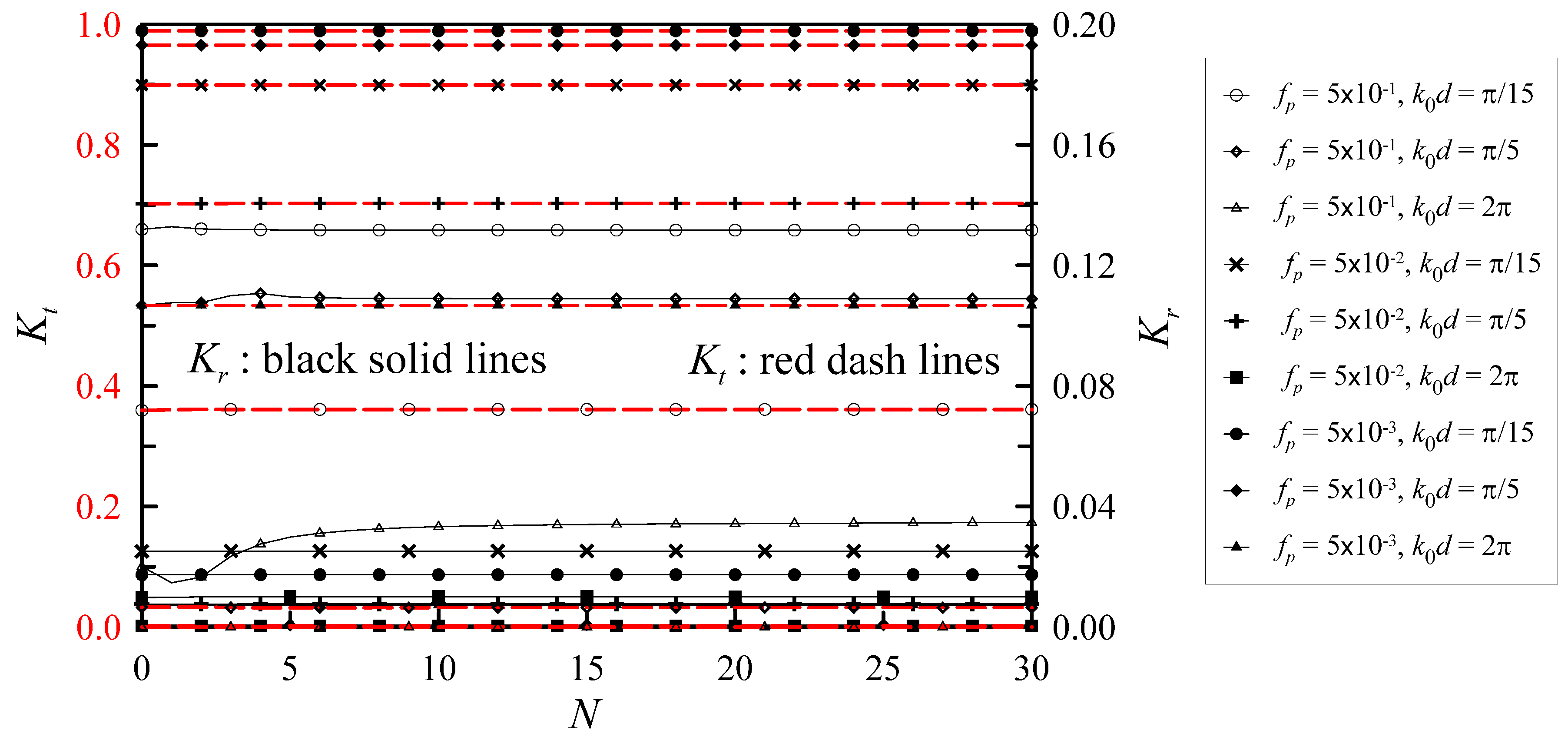
The analytical solutions of water waves comprise evanescent wave sequences and need to determine the number of evanescent modes in the computation. Figure 1 illustrates the computed coefficients of wave reflection and transmission versus the number of evanescent modes used in the study. The computational conditions are listed in

Table 1. Computational conditions for the verification of the number of adopted evanescent modes of the proposed solution.

Computational Conditions		Computational Conditions
$k_{0}d$	π/15 π/5 2π	$f_p$	5 × 10−1 5 × 10−2 5 × 10−3
$H_i/d$	0.01	$b_v$(m)	0.012
$b/d$	1	$N_v$(steams/m2)	194
$h/d$	1.0285	$S$	1
${\rho }_w$ (kg/m3)	1000	${\rho }_s$(kg/m3)	32
$\nu$ (m2/s)	1.12 × 10−6	$n’$	0.98
$\beta$ (m2/N)	4.35 × 10−10	$\mu$	0.333
$G$ (N/m2)	1.29 × 105

. Nine sets of conditions are used in the computation, including combinations of three wave conditions and three linear vegetation friction factors: $k_{0}d=$π/15, π/5, and 2π, and $f_p=$$5\times {10}^{-1}$, $5\times {10}^{-2}$, and $5\times {10}^{-3}$. The results show that the coefficients of wave reflection and transmission can achieve good convergence below ten evanescent modes. In this study, N = 20 is used for subsequent calculations and analysis.

4.2. Modification Factor for Vegetation Friction

The linear vegetation friction factor, $f_p$, is usually determined by experimental calibration or other related energy dissipation formulae. Dalrymple et al. [43] and Mendez and Losada [22] respectively proposed regular and random wave energy attenuation for vegetation as follows:

$${\epsilon }_v=\frac{2}{3\pi }{\rho }_w{C}_D{b}_v{N}_v{\left(\frac{g{k}_0}{2\omega }\right)}^3\frac{{\sinh }^3{k}_{0}d+3\sinh k_{0}d}{3k_0{\cosh }^3{k}_{0}d}{H}^3,$$

(31)

$${\epsilon }_v=\frac{1}{2\sqrt{\pi }}{\rho }_w{C}_D{b}_v{N}_v{\left(\frac{g{k}_0}{2\omega }\right)}^3\frac{{\sinh }^3{k}_{0}d+3\sinh k_{0}d}{3k_0{\cosh }^3{k}_{0}d}{H}_{rms}^3,$$

(32)

where $H$ is the wave height of a regular wave and $H_{rms}$ is the root mean square wave height for a random wave. To evaluate $f_p$ from the energy attenuation formulae of Equations (31) and (32), the modification factor $\hspace{0.17em}{\kappa }_p$ in Equation (9) needs to be estimated, which is related to the characteristic velocity of the wave (the Keulegan–Carpenter number and the ratio of the group wave velocity to the wave velocity $\hspace{0.17em}1/2+k_{0}d/\sinh 2k_{0}d$) and the vegetation parameters ($b$, $b_v$, and $N_v$), as shown in Equation (33)

$${\kappa }_p={\left[{\left(c_0\right)}^{{\lambda }_0}\left(\frac{1}{2}+\frac{k_{0}d}{\sinh 2k_{0}d}\right)\frac{1}{(\mathrm{KC})}\right]}^{{\lambda }_1}{\left(b_v{N}_{v}b\right)}^{{\lambda }_2},$$

(33)

where (KC) is the Keulegan–Carpenter number. $c_0$, ${\lambda }_0$, ${\lambda }_1$, and ${\lambda }_2$ are undetermined coefficients that can be obtained by the double best-fit method according to a large number of case analysis results on the transmission coefficients of the theoretical models of Dalrymple et al. [43] and Mendez and Losada [22], respectively. First, a set of $f_p$ values for each computing case are chosen based on a best fit between the estimation of the present analytical solution and the past theoretical model (Dalrymple et al. [43] or Mendez and Losada [22]). By substituting Equation (33) into Equation (9) and using the best-fit method again, the coefficients in Equation (33) can be obtained; then, the modification factor $\hspace{0.17em}{\kappa }_p$ can be finally expressed as

$${\kappa }_p={\left[{\left(40\right)}^{7/40}\left(\frac{1}{2}+\frac{k_{0}d}{\sinh 2k_{0}d}\right)\frac{1}{(\mathrm{KC})}\right]}^{\frac{1}{3.5}}{\left(b_v{N}_{v}b\right)}^{-1/4}$$

(34)

for regular waves, and

$${\kappa }_p={\left[\frac{3\sqrt{\pi }}{4}{\left(40\right)}^{116/300}\left(\frac{1}{2}+\frac{k_{0}d}{\sinh 2k_{0}d}\right)\frac{1}{(\mathrm{KC})}\right]}^{\frac{1}{2.9}}{\left(b_v{N}_{v}b\right)}^{-1/3}$$

(35)

for random waves ($H_{rms}$).

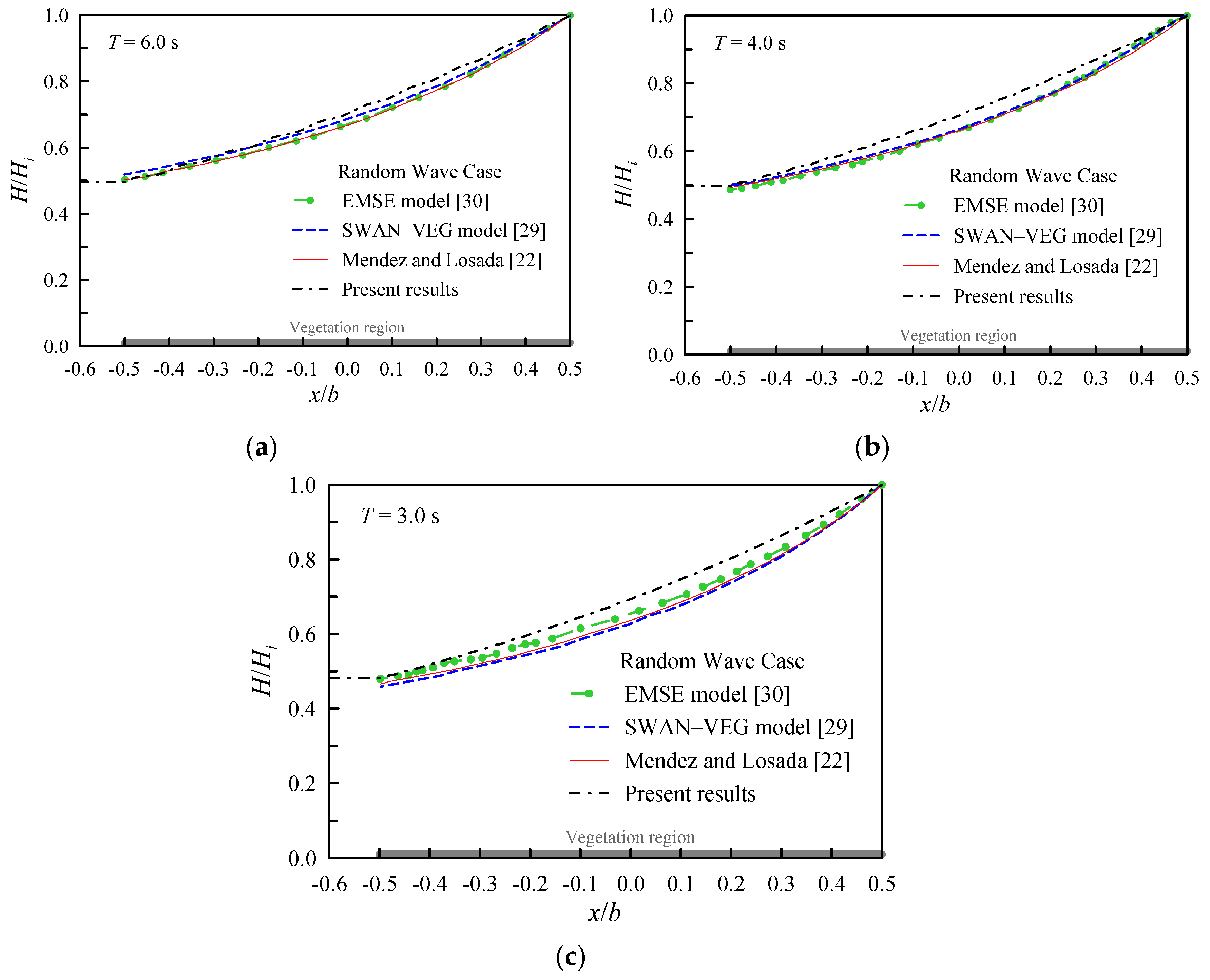
The comparisons of $H/H_i$ between the random waves among the present solution with two numerical models [29,30] and a random wave transformation model [22] are shown in Figure 2 and Figure 3. Both the root mean square error (RMSE) and correlation coefficient (COR) of $K_t$ ($K_t$ is the $H/H_i$ value at the lee side of vegetation) for the proposed solution, based on Mendez and Losada’s theory [22], are computed for comparison, as listed in

Table 2. Root mean square error (RMSE) and correlation coefficient (COR) of $K_t$ for the proposed solution (based on the $K_t$ values obtained by Mendez and Losada [22] shown in Figure 2 and Figure 3).

Statistical Coefficients	Proposed Solution
RMSE of Kt	9.90 × 10−3
COR of Kt	0.996

. The theoretical results of this study are consistent with the wave height in front of and behind the vegetation. It is worth noting that the trend of wave attenuation in the vegetation field calculated from the proposed analytical solution is slightly different from that of Mendez and Losada [22], Suzuki et al. [29], and Cao et al. [30]. The linearization of the Darcy–Weisbach type of vegetation frictional resistance by Lorentz’s hypothesis leads to the non-quadratic dissipation mechanism of wave energy in vegetation fields [45].

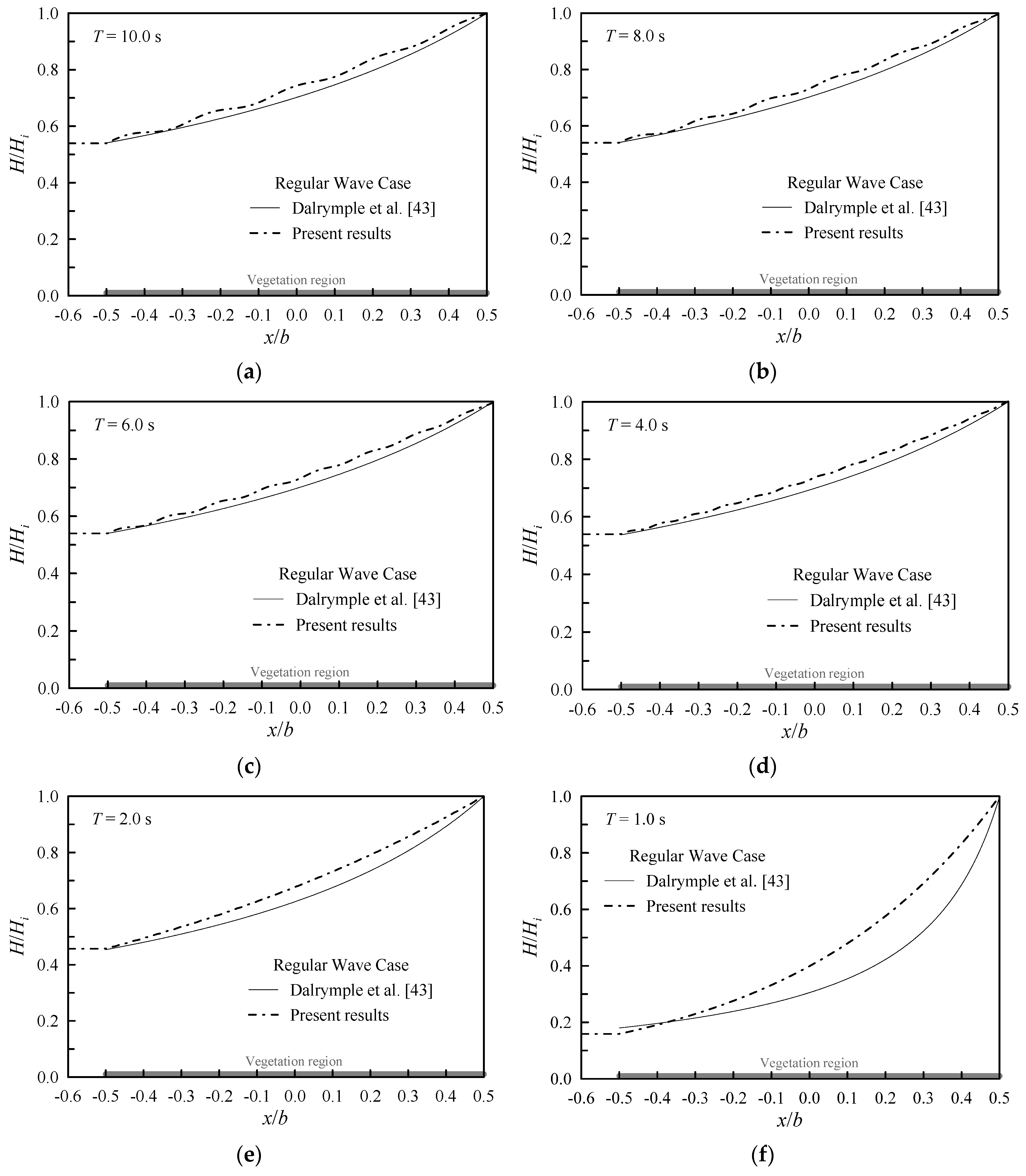
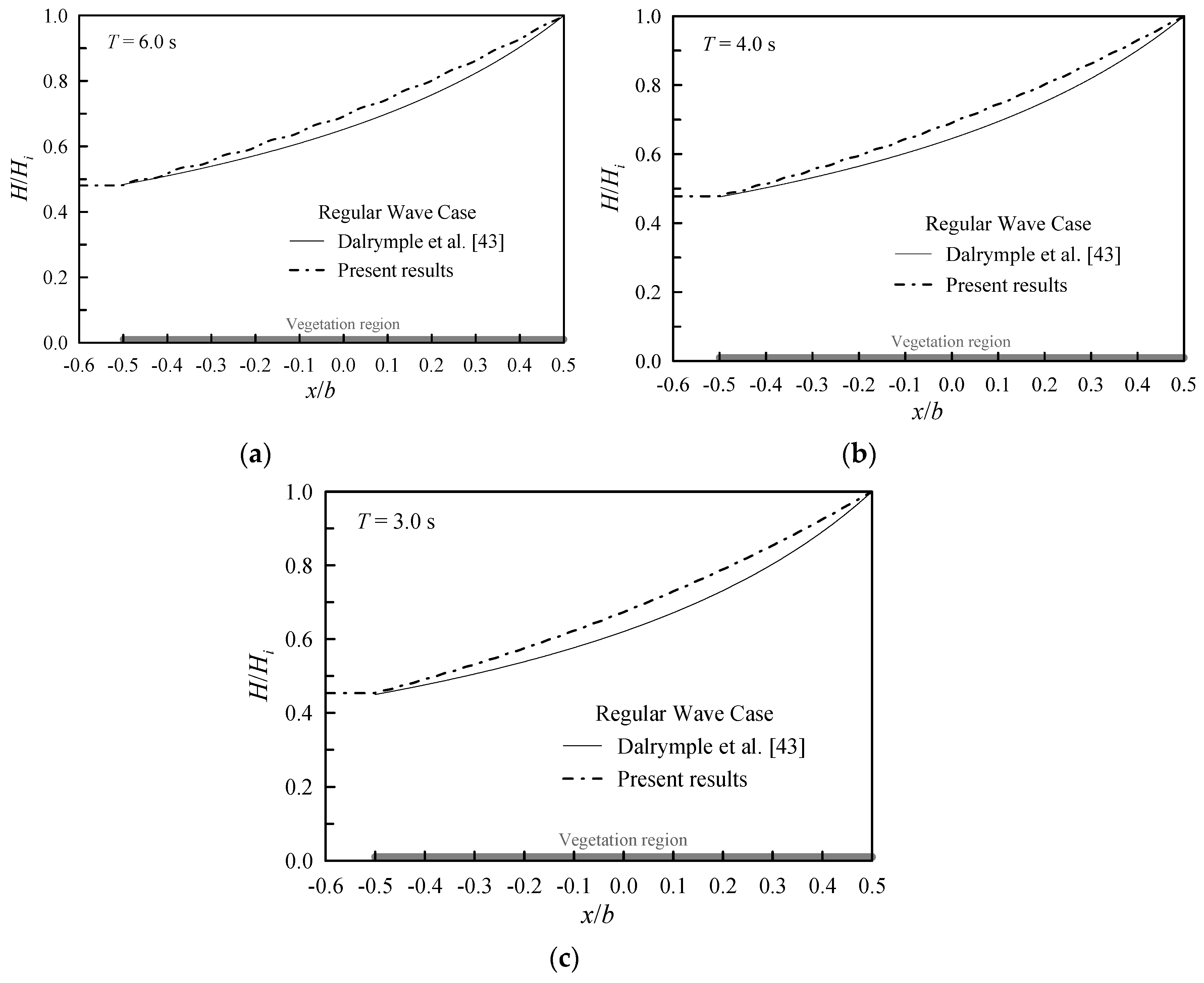
For the regular waves, Figure 4 and Figure 5 show the comparisons of $H/H_i$ between the analytical solution and the regular wave transformation model of Dalrymple et al. [43]. The RMSE and COR coefficients of $K_t$ for the proposed solution are listed in

Table 3. RMSE and COR of $K_t$ for the proposed solution (based on the $K_t$ values obtained by Dalrymple et al. [43] shown in Figure 4 and Figure 5).

Statistical Coefficients	Proposed Solution
RMSE of Kt	7.35 × 10−3
COR of Kt	0.999

. The theoretical results of this study are also consistent with the wave heights in front of and behind vegetation fields.

4.3. Effect of the Drag Coefficient of Vegetation

The drag coefficient, $C_D$, owing to the effect of emergent vegetation, is generally related to the characteristics of the plant (geometry, stem density, spatial coverage, buoyancy, stiffness, etc.) and the hydrodynamic conditions (water depth, wave period, wave height, etc.). To investigate the influence of the drag coefficient of the emergent vegetation, the set of input conditions of water waves and vegetation used for the computations were $H_i/d=$ 0.3; $d=$ 0.3 m; $b/d=$ 20; $h/d=$ 1.0285; $b_v=$ 0.012 m; $N_v=$ 194 steams/m²; $S=$ 1; $\mu =$ 0.333; $n’=$ 0.999; ${\rho }_s=$ 600 kg/m³; ${\rho }_w=$ 1000 kg/m³; $\nu =$ 1.12 × ${10}^{-6}$ m²/s; $\beta =$ 4.35 × ${10}^{-10}$ m²/N; $G=$ 1.29 × ${10}^5$ N/m²; and $C_D=$ 0.5, 1.0, 1.5, and 2.0. The variations in $K_r$ and $K_t$, and the energy dissipation, $E_f$, as a function of $k_{0}d$ for $C_D$, are revealed in Figure 6. The wave reflection is marginal, and the reflectance is only slightly increased when the wave condition, $k_{0}d$, is less than 1.5. This is mainly because the vegetation is highly permeable and most of the wave energy passes through the vegetation. As $k_{0}d$ decreases (towards shallow-water conditions), the wave transmission increases gradually and then tends to reach a certain value, and the wave energy dissipates gradually and then tends to reach a constant value. In addition, as the drag coefficient, $C_D$, increases, the wave energy dissipation, $E_f$, increases, and the wave transmission, $K_t$, decreases.

4.4. Effect of the Plant Stem Diameter of Vegetation

Figure 7 shows the reflection, transmission, and energy dissipation with the plant stem diameter, $b_v=$ 0.012, 0.024, 0.036, and 0.048 m, when the drag coefficient, $C_D$, is equal to 1. The remaining input conditions of the water waves and vegetation are the same as in Figure 6. It is shown that that even if the vegetation drag coefficient is constant, as the stem diameter increases, the wave is hindered by the plants and induces larger energy dissipation in the vegetation field, resulting in a decrease in the wave transmission.

4.5. Effect of the Stem Density of Vegetation

Figure 8 reveals the reflection, transmission and energy dissipation with the stem density $N_v=$ 48.5, 97, 194, and 388 steams/m². The drag coefficient, $C_D=1$, and the remaining input conditions of water waves and vegetation are the same as in Figure 6. The results show that as the stem density increases, the denser flora affect waves passing through the vegetation fields, causing more energy dissipation and resulting in a decrease in the wave transmission.

4.6. Effect of the Spatial Coverage of Vegetation

It is well-known that as the width of vegetation increases, the distance of the hindering wave propagation increases, causing more energy dissipation and resulting in a decrease in the wave transmission [22,43]. The larger the dimensionless width, the smaller the average energy dissipation per unit width. Figure 9 reveals the above result. The input conditions of dimensionless width in Figure 9 are $b/d=$ $20/3$, $40/3$, $20$, and $80/3$. The remaining input conditions are $H_i/d=$ 0.3, $d=$ 0.3 m, $h/d=$ 1.0285, $b_v=$ 0.012 m, $N_v=$ 194 steams/m², $S=$ 1, $\mu =$ 0.333, $n’=$ 0.999, ${\rho }_s=$ 600 kg/m³, ${\rho }_w=$ 1000 kg/m³, $\nu =$ 1.12 × ${10}^{-6}$ m²/s, $\beta =$ 4.35 × ${10}^{-10}$ m²/N, $G=$ 1.29 × ${10}^5$ N/m², and $C_D=1.0$.

4.7. Applicability of Different Vegetation Stiffness

Flexible plants have the ability to change shape to reduce drag by reducing the cross-sectional area perpendicular to the flow [18]. In general, the drag ($F_D$) of a plant is proportional to a power of the $Q_x$:

$$F_D=\frac{1}{2}{\rho }_w{C}_D{b}_v{N}_v{\left(Q_x\right)}^{\gamma },$$

(36)

with $\gamma =2$ for rigid plants (Darcy–Weisbach configuration), but $\gamma <2$ for flexible plants [18,46]. The proposed analytical solution is theoretically applicable to rigid vegetation (and has been proven in Section 4.2). However, it is necessary to discuss whether the analysis model can be practically applied to emergent vegetation cases with different stiffnesses.

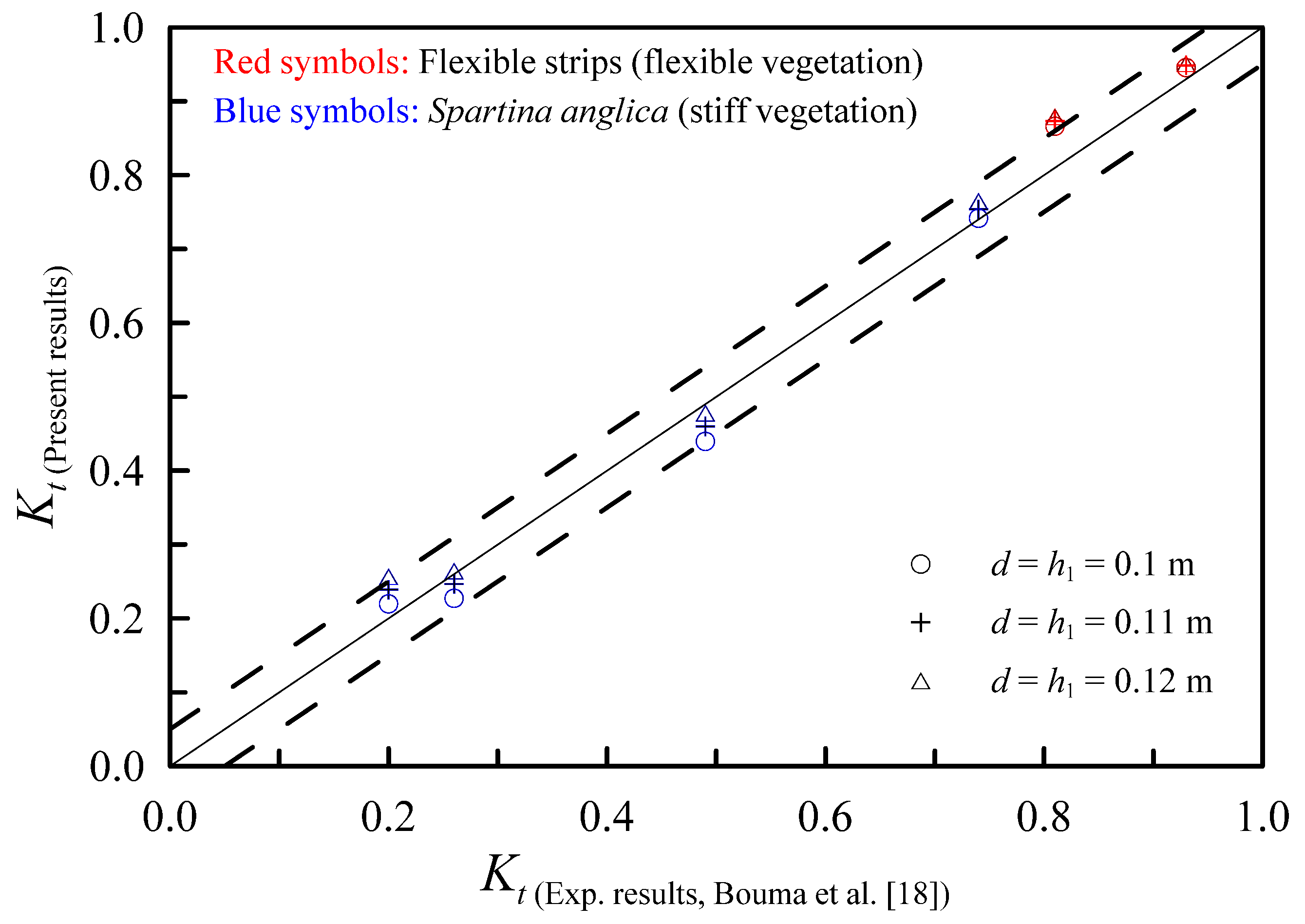
Figure 10 reveals a corresponding comparison of the transmission coefficient $K_t$ obtained in the experimental results of Bouma et al. [18] and the present computations. The physical properties of plant characteristics and wave data for experimentation are listed in

Table 4. Physical properties of plant characteristics and wave data for experimentation.

Vegetation Type	tv(m) †	bv(m)	CD ‡	Nv (Stems/m2)	b(m)	d(m)	Incident Wave Data		Kt
							Hrms(m)	T(s)
Flexible
Flexible strips	0.1	0.04	4.244 × 10−2	450	2	0.12	0.032	1.0	0.93
Flexible strips	0.1	0.04	4.244 × 10−2	1850	2	0.12	0.032	1.0	0.81
Stiff
Spartina anglica	0.1	0.192	1.3794 × 10−1	225	2	0.12	0.028	1.0	0.74
Spartina anglica	0.1	0.192	1.3794 × 10−1	900	2	0.12	0.032	1.0	0.49
Spartina anglica	0.1	0.192	1.3794 × 10−1	2400	2	0.12	0.029	1.0	0.26
Spartina anglica	0.1	0.192	1.3794 × 10−1	2400	2	0.12	0.030	1.0	0.20

† t_v is the height of vegetation. ‡ The C_D values are unit-corrected values from Table 2 of Bouma et al. [18].

. The experiment of Bouma et al. belongs to the wave attenuation experiment on near-emergent vegetation (because the vegetation height is slightly lower than the water depth in the experimental observation section). The vegetation height must be equal to the water depth for the present analytical solution, so three scenarios ($d=h_1=$ 0.1, 0.11, and 0.12 m) were computed for comparison. The horizontal and vertical coordinate components of the points in Figure 10 respectively represent the wave transmission coefficient of experimentation (K_{t (Exp. Results, Boumaet al. [18])}) and that of the present computation (K_{t (Present results)}). The points would coincide with the solid oblique line in Figure 10 when K_{t (Present results)} = K_{t (Exp. Results, Boumaet al. [18])}. The range of dashed lines indicates that the calculation error of K_t is within 5%, which is generally the allowable range in practical applications. Figure 10 shows reasonable comparison results, indicating that the proposed analytical solution can be applied to the analysis of practical cases, including the condition of flexible vegetation.

5. Conclusions

In this paper, an analytical solution for waves propagating through an emergent vegetation medium is presented. A vegetation theory based on Lan–Lee’s poro-elastomer theory and a linearized Darcy–Weisbach type of friction resistance is proposed and developed. The interactions between the waves and the emergent vegetation medium are considered using continuities of flow flux and pressure on the interfacial boundaries. The free surface boundary conditions in the field of emergent vegetation medium are also considered in the study. According to the wave energy dissipation by Dalrymple et al. [43] and Mendez and Losada [22], a parameter estimation formula for the linear vegetation friction factor can be determined through a best-fit process. The results compared reasonably with the computing cases of Suzuki et al. [29] and Cao et al. [30] for random waves and with the wave transformation model of Mendez and Losada [22] for regular wave cases. Wave reflection, transmission, and attenuation induced from the emergent vegetation were studied, including the effects of the drag coefficient, plant stem diameter, stem density, and spatial coverage. The results show that when the other influencing factors are fixed, an increase in the drag coefficient, stem diameter, stem density, or spatial coverage results in the emergency vegetation increasing the wave energy dissipation and reducing the wave transmission. As the incident waves move to shallow-water conditions, the wave transmission gradually increases and then tends to reach a certain value, and the wave dissipation shows the opposite trend. Vegetation stiffness is an essential factor affecting the drag coefficient. Study of the empirical formula for the drag coefficient needs to take the vegetation stiffness into account.

The present theory and solution provide an economic and general way to pre-investigate problems of wave transformation through emergent vegetation (including flexible plants), under the precondition that the linear vegetation friction factor has been determined. The applications include a system study of the waves passing through a group of vegetation, as well as the development of a wave absorber based on a combination of hydraulic/ocean engineering and biology.

References

- Koch, E.W.; Sanford, L.P.; Chen, S.-N.; Shafer, D.J.; McKee, S.J. Waves in Seagrass Systems: Review and Technical Recommendations; U.S. Army Corps of Engineers: Washington, DC, USA, 2006.
- Neumeier, U.; Ciavola, P. Flow Resistance and Associated Sedimentary Processes in a Spartina maritima Salt-Marsh. J. Coast. Res. 2004, 202, 435–447. [Google Scholar] [CrossRef]
- Choi, S.-U.; Kang, H. Reynolds stress modeling of vegetated open-channel flows. J. Hydraul. Res. 2004, 42, 3–11. [Google Scholar] [CrossRef]
- Li, C.; Yan, K. Numerical Investigation of Wave–Current–Vegetation Interaction. J. Hydraul. Eng. 2007, 133, 794–803. [Google Scholar] [CrossRef]
- Dimitris, S.; Prinos, P. Macroscopic Turbulence Models and Their Application in Turbulent Vegetated Flows. J. Hydraul. Eng. 2011, 137, 315–332. [Google Scholar] [CrossRef]
- Ghisalberti, M. Mixing layers and coherent structures in vegetated aquatic flows. J. Geophys. Res. Space Phys. 2002, 107, 3011. [Google Scholar] [CrossRef]
- Poggi, D.; Porporato, A.; Ridolfi, L.; Albertson, J.; Katul, G.G. The Effect of Vegetation Density on Canopy Sub-Layer Turbulence. Bound. Layer Meteorol. 2004, 111, 565–587. [Google Scholar] [CrossRef]
- Folkard, A. Hydrodynamics of model Posidonia oceanica patches in shallow water. Limnol. Oceanogr. 2005, 50, 1592–1600. [Google Scholar] [CrossRef]
- Ciraolo, G.; Ferreri, G.B.; La Loggia, G. Flow resistance of Posidonia oceanica in shallow water. J. Hydraul. Res. 2006, 44, 189–202. [Google Scholar] [CrossRef]
- Luhar, M.; Rominger, J.; Nepf, H. Interaction between flow, transport and vegetation spatial structure. Environ. Fluid Mech. 2008, 8, 423–439. [Google Scholar] [CrossRef]
- Ghisalberti, M.; Nepf, H. Shallow Flows Over a Permeable Medium: The Hydrodynamics of Submerged Aquatic Canopies. Transp. Porous Media 2009, 78, 385–402. [Google Scholar] [CrossRef]
- Suzuki, T.; Arikawa, T. Numerical Analysis of bulk drag coefficient in dense vegetation by immersed boundary method. In Proceedings of the 32nd Conference on Coastal Engineering, Shanghai, China, 30 June–5 July 2011. [Google Scholar] [CrossRef]
- Stratigaki, V.; Manca, E.; Prinos, P.; Losada, I.; Lara, J.; Sclavo, M.; Amos, C.L.; Cáceres, I.; Sánchez-Arcilla, A. Large-scale experiments on wave propagation over Posidonia oceanica. J. Hydraul. Res. 2011, 49, 31–43. [Google Scholar] [CrossRef]
- Asano, T.; Deguchi, H.; Kobayashi, N. Interaction between Water Waves and Vegetation. Coast. Eng. 1993, 3, 2709–2723. [Google Scholar]
- Möller, I.; Spencer, T.; French, J.; Leggett, D.; Dixon, M. Wave Transformation Over Salt Marshes: A Field and Numerical Modelling Study from North Norfolk, England. Estuar. Coast. Shelf Sci. 1999, 49, 411–426. [Google Scholar] [CrossRef]
- Fonseca, M.S.; Cahalan, J.A. A preliminary evaluation of wave attenuation by four species of seagrass. Estuar. Coast. Shelf Sci. 1992, 35, 565–576. [Google Scholar] [CrossRef]
- Ota, T.; Kobayashi, N.; Kirby, J.T.; Smith, J.M. Wave and current interactions with vegetation. In Coastal Engineering; World Scientific Pub Co Pte Ltd.: Singapore, 2005; pp. 508–520. [Google Scholar]
- Bouma, T.; De Vries, M.B.; Low, E.; Peralta, G.; Tanczos, I.C.; Van De Koppel, J.; Herman, P.M.J. Trade-OFFS Related to ecosystem engineering: A case study on stiffness of emerging macrophytes. Ecology 2005, 86, 2187–2199. [Google Scholar] [CrossRef] [Green Version]
- Lima, S.F.; Neves, C.F.; Rosauro, N.M.L.; Smith, J.M. Damping of gravity waves by fields of flexible vegetation. Coast. Eng. 2007, 1, 491–503. [Google Scholar]
- John, B.M.; Shirlal, K.G.; Rao, S. Effect of artificial vegetation on wave attenuation-An experimental investigation. Procedia Eng. 2015, 116, 600–606. [Google Scholar] [CrossRef] [Green Version]
- Anderson, M.E.; Smith, J.M.; McKay, S.K. Wave Dissipation by Vegetation; Coastal and Hydraulics Engineering Technical Note ERDC/CHL CHETN–I–82, US Army Engineer Research and Development Center Coastal and Hydraulics Laboratory Vicksburg United States: Vicksburg, MS, USA, 2011. [Google Scholar]
- Mendez, F.J.; Losada, I. An empirical model to estimate the propagation of random breaking and nonbreaking waves over vegetation fields. Coast. Eng. 2004, 51, 103–118. [Google Scholar] [CrossRef]
- Suzuki, T.; Dijkstra, J. Wave propagation over strongly varying topography: Cliffs and vegetation. In Proceedings of the 32nd International Association for Hydraulic Research-The Congress, Venice, Italy, 1–6 July 2007. [Google Scholar]
- Dubi, A. Damping of Water Waves by Submerged Vegetation: A Case Study on Laminaria Hyperborea. Ph.D. Thesis, University of Trondheim, Trondheim, Norway, 1995. [Google Scholar]
- Løvås, S.M.; Tørum, A. Effect of the kelp Laminaria hyperborea upon sand dune erosion and water particle velocities. Coast. Eng. 2001, 44, 37–63. [Google Scholar] [CrossRef]
- Lopez, F.; Garcia, M. Open Channel Flow through Simulated Vegetation: Turbulence Modelling and Sediment Transport; WRP-CP 10; US Army Engineer Waterways Experiment Station: Vicksburg, MI, USA, 1997. [Google Scholar]
- Asano, T.; Tsutsui, S.; Sakai, T. Wave damping characteristics due to seaweed. In Proceedings of the 35th Coastal Engineering Conference; Japan Society of Civil Engineers: Tokyo, Japan, 1988; pp. 138–142. [Google Scholar]
- Dean, R.G.; Bender, C.J. Static wave setup with emphasis on damping effects by vegetation and bottom friction. Coast. Eng. 2006, 53, 149–156. [Google Scholar] [CrossRef]
- Suzuki, T.; Zijlema, M.; Burger, B.; Meijer, M.C.; Narayan, S. Wave dissipation by vegetation with layer schematization in SWAN. Coast. Eng. 2012, 59, 64–71. [Google Scholar] [CrossRef]
- Cao, H.; Feng, W.; Hu, Z.; Suzuki, T.; Stive, M.J.F. Numerical modeling of vegetation-induced dissipation using an extended mild-slope equation. Ocean Eng. 2015, 110, 258–269. [Google Scholar] [CrossRef]
- Yamamoto, T. On the response of a Coulomb-damped poroelastic bed to water waves. Mar. Geotechnol. 1983, 5, 93–130. [Google Scholar] [CrossRef]
- Huang, L.H.; Song, C.H. Dynamic Response of Poroelastic Bed to Water Waves. J. Hydraul. Eng. 1993, 119, 1003–1020. [Google Scholar] [CrossRef]
- Hsieh, P.C.; Huang, L.H.; Wang, T.W. Dynamic response of soft poroelastic bed to nonlinear water wave—Boundary layer correction approach. J. Eng. Mech. 2000, 126, 1064–1073. [Google Scholar] [CrossRef]
- Lin, M.; Jeng, D. Comparison of existing poroelastic models for wave damping in a porous seabed. Ocean Eng. 2003, 30, 1335–1352. [Google Scholar] [CrossRef] [Green Version]
- Lan, Y.-J.; Lee, J.-F. On waves propagating over a submerged poro-elastic structure. Ocean Eng. 2010, 37, 705–717. [Google Scholar] [CrossRef]
- Lan, Y.; Hsu, T.-W.; Lai, J.; Chang, C.; Ting, C. Bragg scattering of waves propagating over a series of poro-elastic submerged breakwaters. Wave Motion 2011, 48, 1–12. [Google Scholar] [CrossRef]
- Lan, Y.J.; Hsu, T.W.; Liu, Y.R. Analysis of wave interaction with an adjoining–type of composite poro–elastic submerged breakwater. In Proceedings of the 23rd International Offshore and Polar Engineering Conference, Anchorage, AK, USA, 30 June–4 July 2013; pp. 1152–1159. [Google Scholar]
- Lan, Y.; Hsu, T.; Liu, Y. Mathematical study on wave interaction with a composite poroelastic submerged breakwater. Wave Motion 2014, 51, 1055–1070. [Google Scholar] [CrossRef]
- Lan, Y.-J.; Hsu, T.-W.; Gan, F.-X.; Li, C.-Y. Mathematical study of wave interaction with a mound type of composite poroelastic submerged breakwater. Ocean Eng. 2016, 124, 1–12. [Google Scholar] [CrossRef]
- Biot, M.A. Theory of propagation elastic waves in a fluid saturated porous solid. I. low–frequency range. J. Acoust. Soc. Am. 1956, 28, 168–178. [Google Scholar] [CrossRef]
- Sollitt, C.K.; Cross, R.H. Wave transmission through permeable breakwaters. In Proceedings of the 13th International Conference on Coastal Engineering, Vancouver, BC, Canada, 10–14 July 1972; p. 99. [Google Scholar] [CrossRef]
- Lan, Y.J. On waves propagating through an emergent poroelastic medium. J. Mar. Sci. Technol. 2019, 27, 377–391. [Google Scholar]
- Dalrymple, R.; Kirby, J.T.; Hwang, P. Wave Diffraction Due to Areas of Energy Dissipation. J. Waterw. Port Coast. Ocean Eng. 1984, 110, 67–79. [Google Scholar] [CrossRef]
- Nepf, H.M. Drag, turbulence, and diffusion in flow through emergent vegetation. Water Resour. Res. 1999, 35, 479–489. [Google Scholar] [CrossRef]
- Lan, Y.J. Analytical solution of wave damping by flexible emergent vegetation. In Proceedings of the 9th Chinese-German Joint Symposium on Hydraulic and Ocean Engineering (CGJOINT 2018), Tainan, Taiwan, 11–17 November 2018; pp. 155–165. [Google Scholar]
- Sand-Jensen, K. Drag and reconfiguration of freshwater macrophytes. Freshw. Biol. 2003, 48, 271–283. [Google Scholar] [CrossRef]
Figure 1.
Comparison of the reflection and transmission coefficients versus the number of adopted evanescent wave modes.
Figure 2.
Comparison of evolution in the vegetation region for the present analytical solution, SWAN–VEG numerical model [29], and random wave transformation model of Mendez and Losada [22] ( 0.4 m, 2 m, 100 m, 0.04 m, 10 steams/m2, 1, 1, 0.333, 0.999, 681.43 kg/m3, 1000 kg/m3, 1.12 × m2/s, 4.35 × m2/N, and 1.29 × N/m2). (a) T = 10 s; (b) T = 8 s; (c) T = 6 s; (d) T = 4 s; (e) T = 2 s; (f) T = 1 s.
Figure 3.
Comparison of evolution in the vegetation region for the present analytical solution, numerical wave models [29,30], and random wave transformation model [22] ( 0.2 m, 3 m, 150 m, 1 m, 1 steam/m2, 1, 1, 0.333, 0.999, 681.43 kg/m3, 1000 kg/m3, 1.12 × m2/s, 4.35 × m2/N, and 1.29 × N/m2). (a) T = 6 s; (b) T = 4 s; (c) T = 3 s.
Figure 4.
Comparison of evolution in the vegetation region for the present analytical solution and regular wave transformation model of Dalrymple et al. [43] ( 0.4 m, 2 m, 100 m, 0.04 m, 10 steams/m2, 1, 1, 0.333, 0.999, 681.43 kg/m3, 1000 kg/m3, 1.12 × m2/s, 4.35 × m2/N, and 1.29 × N/m2). (a) T = 10 s; (b) T = 8 s; (c) T = 6 s; (d) T = 4 s; (e) T = 2 s; (f) T = 1 s.
Figure 5.
Comparison of evolution in the vegetation region for the present analytical solution and regular wave transformation model of Dalrymple et al. [43] ( 0.2 m, 3 m, 150 m, 1 m, 1 steam/m2, 1, 1, 0.333, 0.999, 681.43 kg/m3, 1000 kg/m3, 1.12 × m2/s, 4.35 × m2/N, and 1.29 × N/m2). (a) T = 6 s; (b) T = 4 s; (c) T = 3 s.
Figure 6.
Effect of the drag coefficient of vegetation on , , and ( 0.3, 0.3 m, 20, 1.0285, 0.012 m, 194 steams/m2, 1, 0.333, 0.999, 600 kg/m3, 1000 kg/m3, 1.12 × m2/s, 4.35 × m2/N, and 1.29 × N/m2).