Predicting the Trend of Dissolved Oxygen Based on the kPCA-RNN Model


1
Agriculture & Food, CSIRO, Brisbane, QLD 4067, Australia
2
Land & Water, CSIRO, Canberra, ACT 2601, Australia
*
Author to whom correspondence should be addressed.
Water 2020, 12(2), 585; https://doi.org/10.3390/w12020585
Submission received: 19 December 2019
/
Revised: 10 February 2020
/
Accepted: 14 February 2020
/
Published: 20 February 2020
(This article belongs to the Special Issue Land Use and Water Quality)
Abstract
:Water quality forecasting is increasingly significant for agricultural management and environmental protection. Enormous amounts of water quality data are collected by advanced sensors, which leads to an interest in using data-driven models for predicting trends in water quality. However, the unpredictable background noises introduced during water quality monitoring seriously degrade the performance of those models. Meanwhile, artificial neural networks (ANN) with feed-forward architecture lack the capability of maintaining and utilizing the accumulated temporal information, which leads to biased predictions in processing time series data. Hence, we propose a water quality predictive model based on a combination of Kernal Principal Component Analysis (kPCA) and Recurrent Neural Network (RNN) to forecast the trend of dissolved oxygen. Water quality variables are reconstructed based on the kPCA method, which aims to reduce the noise from the raw sensory data and preserve actionable information. With the RNN’s recurrent connections, our model can make use of the previous information in predicting the trend in the future. Data collected from Burnett River, Australia was applied to evaluate our kPCA-RNN model. The kPCA-RNN model achieved scores up to 0.908, 0.823, and 0.671 for predicting the concentration of dissolved oxygen in the upcoming 1, 2 and 3 hours, respectively. Compared to current data-driven methods like Feed-forward neural network (FFNN), support vector regression (SVR) and general regression neural network (GRNN), the predictive accuracy of the kPCA-RNN model was at least 8%, 17% and 12% better than the comparative models in these three cases. The study demonstrates the effectiveness of the kPAC-RNN modeling technique in predicting water quality variables with noisy sensory data.
1. Introduction
Surface water quality has a strong dependence on the nature and extent of agricultural, industrial and other anthropogenic activities within a region’s catchments [1]. The reliable prediction of water quality is crucial in order for decision-makers to improve water quality management and protection activities [2]. However, forecasting the temporal variation of water quality parameters for surface river system can be a significantly challenging task owing to rapidly changing environmental conditions and insufficiently historical data records [3].
Dissolved oxygen (DO) content is one of the most vital water quality variables as it directly indicates the status of the aquatic ecosystem and its ability to sustain aquatic life [4]. Rapid decomposition of organic materials, including manure or wastewater sources, can quickly take the DO out of water in few hours, resulting in deficient DO levels that can lead to stress and death of aquatic fauna [5]. For example, DO levels that remain below 1–2 mg/L for a few hours can result in large fish kills. In pond management, an aeration system can quickly increase dissolved oxygen levels if the decreasing of dissolved oxygen in the water can be predicted. Hence, short-term predictions of DO are critical in delivering good water quality management [6].
Various mechanism models have been applied for predicting the concentration of DO [7]. The mechanism model considers many factors such as physical, chemical, and biological factors affecting the change of water quality. The common mechanism models include the BASINS model system [8], the MIKE model system [9], and the QUAL2K model system [10]. However, it is often challenging to simulate the target water quality systems when lacking adequate monitoring data or background information [11]. Consequently, those models are not likely to be able to be generalized without significant parameter adjustment [12].
Data-driven models have received increasing attention in predicting the concentration of DO based on the sensory data. For example, in the study proposed by Zhang [13], a multi-layer feedforward neural network (FFNN) is designed for predicting the trend of dissolved oxygen of the Baffle Creek in Australia. In their approach, a mutual information-based feature selection strategy is introduced to pick up the relevant water quality variables for DO forecasting. Antanasijević et al. [14] tested the effectiveness of applying general regression neural network (GRNN) models for the forecasting of DO in the Danube River, Europe. In their experiments, 19 water quality parameters, five different data normalization methods, and three input selection techniques were tested to find the best combination. In addition, Li et al. [15] evaluated the performance of support vector regression (SVR) for the prediction of DO concentration based on multiple water quality parameters. The SVR was optimized by the particle swarm optimization algorithm and achieved superior performance than linear regression models. Though various data-driven models have been tested in predicting the trend of DO, most existing models lack the mechanisms in processing temporal data. Under these circumstances, seasonal or diurnal patterns within the water quality data are hard to be captured [16].
Apart from model architectures, the quality of input data also has an enormous influence on the data-driven model’s performance [17]. The high-frequency data collected by sensors are prevalent in building water quality forecasting models. However, random errors generated by the environment, instruments or network transmission are unavoidable when monitoring water quality variables [18,19]. Though techniques such as z-score and min-max are used in preprocessing input data for data-driven models [14], those techniques aim to rescale the numeric range of water quality variables instead of reducing sensor noise. Accordingly, the unwanted noise would be accepted by the data-driven models, which increases the challenges for generating accurate predictions for water quality variables.
In this paper, we propose a water quality predictive model based on Kernel Principal Component Analysis (kPCA) and Recurrent Neural Network (RNN) to solve the above issues. Our work differs from other comparative approaches in the following two aspects:
- Kernel Principal Component Analysis (kPCA) is implemented to reconstruct the input water quality data. Instead of feeding the water quality sensor data into the data-driven models directly, we pick up the top-ranked principal components as the new inputs. Meanwhile, the dropped principal components are expected to contain background noise. In this way, the reconstructed inputs only have useful information included.
- A recurrent neural network (RNN) is designed to capture the temporal variations within water quality variables and utilize the historical changing patterns as a guide for predicting water quality in the future.
This study aims to evaluate the predictive accuracy of the kPCA-RNN model by comparing it with three data-driven methods discussed above. The evaluation is undertaken on a case study of DO concentrations in Burnett River, Australia.
2. Material and Methods
2.1. Study Area and Monitoring Data
2.1.1. Overview
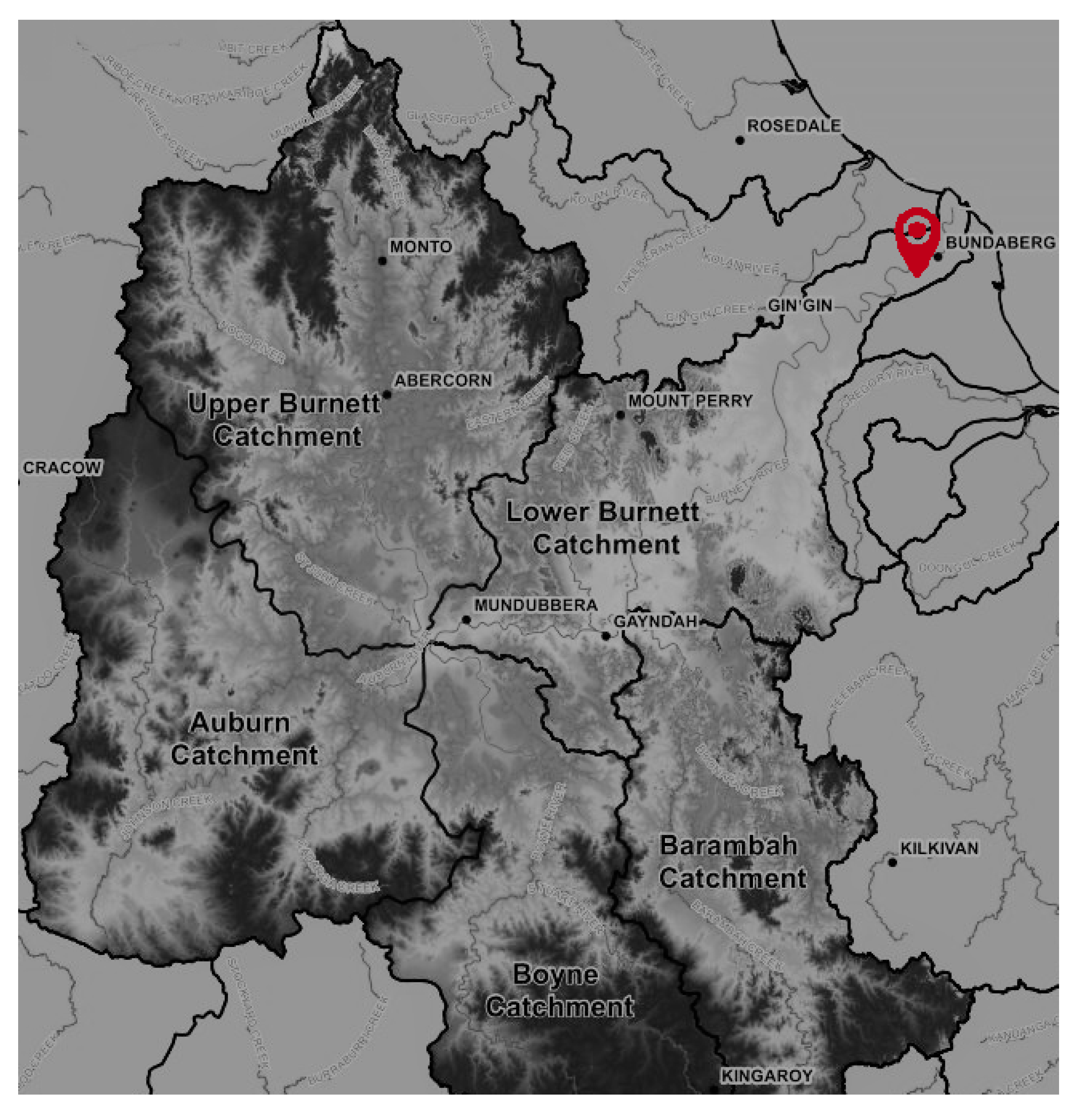
The Burnett River is located on the southern Queensland coast and flows into the coral sea of the South Pacific Ocean. Cultivation of sugar cane and small crops are important land uses in this region. The total area of the catchment is about 33,000 km2. Figure 1 illustrates the location and extent of the catchment. Time series physiochemical water quality variables analysed in this study were obtained by a YSI 6 Series sonde sensor near the Bundaberg Co-op Wharf (Figure 1) [20]. Water quality variables such as temperature, electric conductivity (EC), pH, dissolved oxygen (DO), turbidity, and chlorophyll-a (Chl-a) are recorded with 1 h time interval for 5 months in 2015 (Table 1).
2.1.2. Water Quality Statistical Analysis
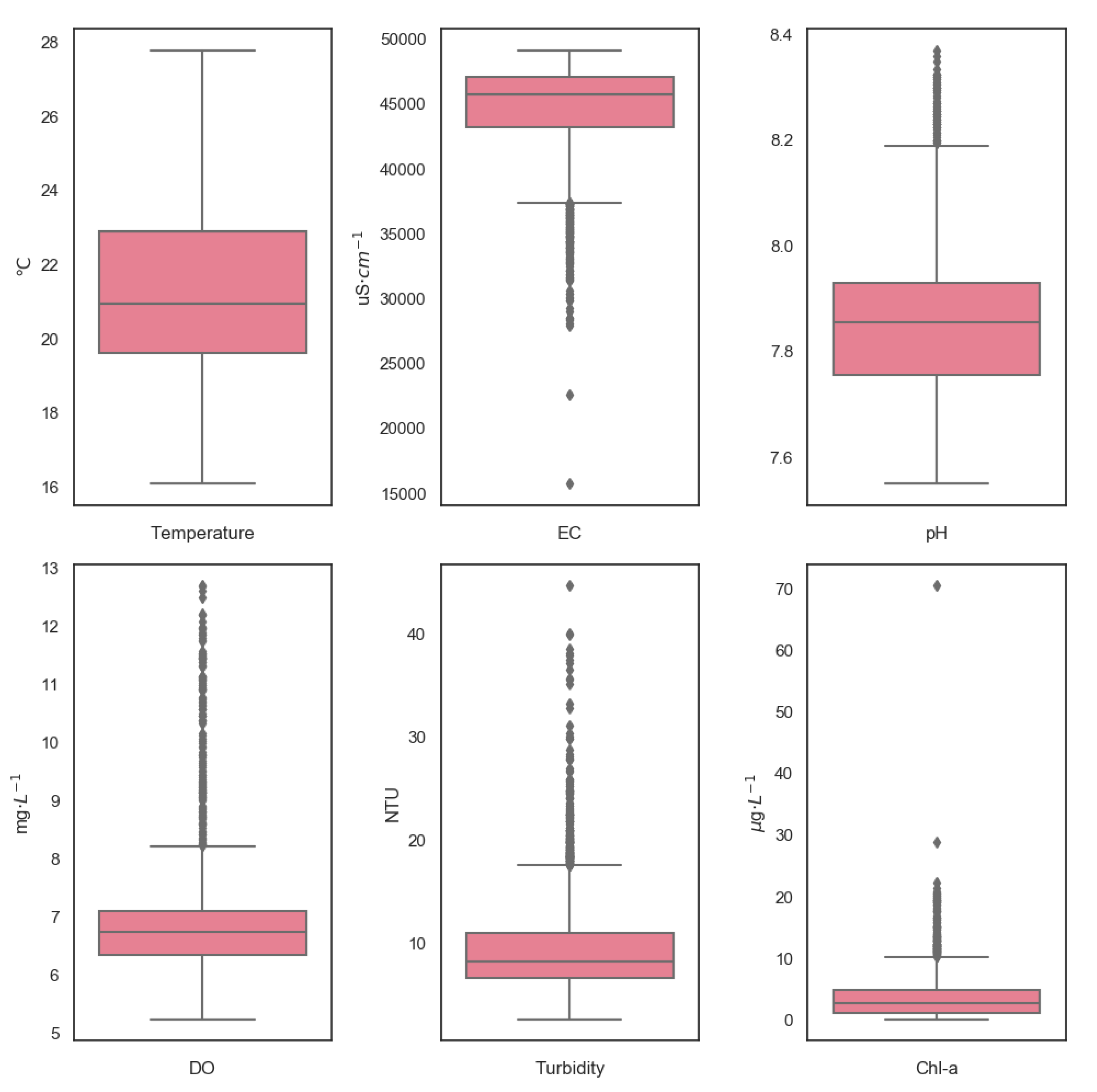
As demonstrated in Table 1, Chl-a and turbidity have larger variability than other water quality variables (CV ). In the case of turbidity, this is due to extreme weather events [22]. The variability of Chl-a concentration can be affected by the discharge of river, temperature, and salinity variation. The high variability in turbidity and Chl-a are caused by a small number of observations with high values (Figure 2). Additionally, outliers of EC tend to have lower measurement values. These outliers can be caused by variations in river flow of other characteristics of the catchment. Ignoring those variations may cause serious information loss.
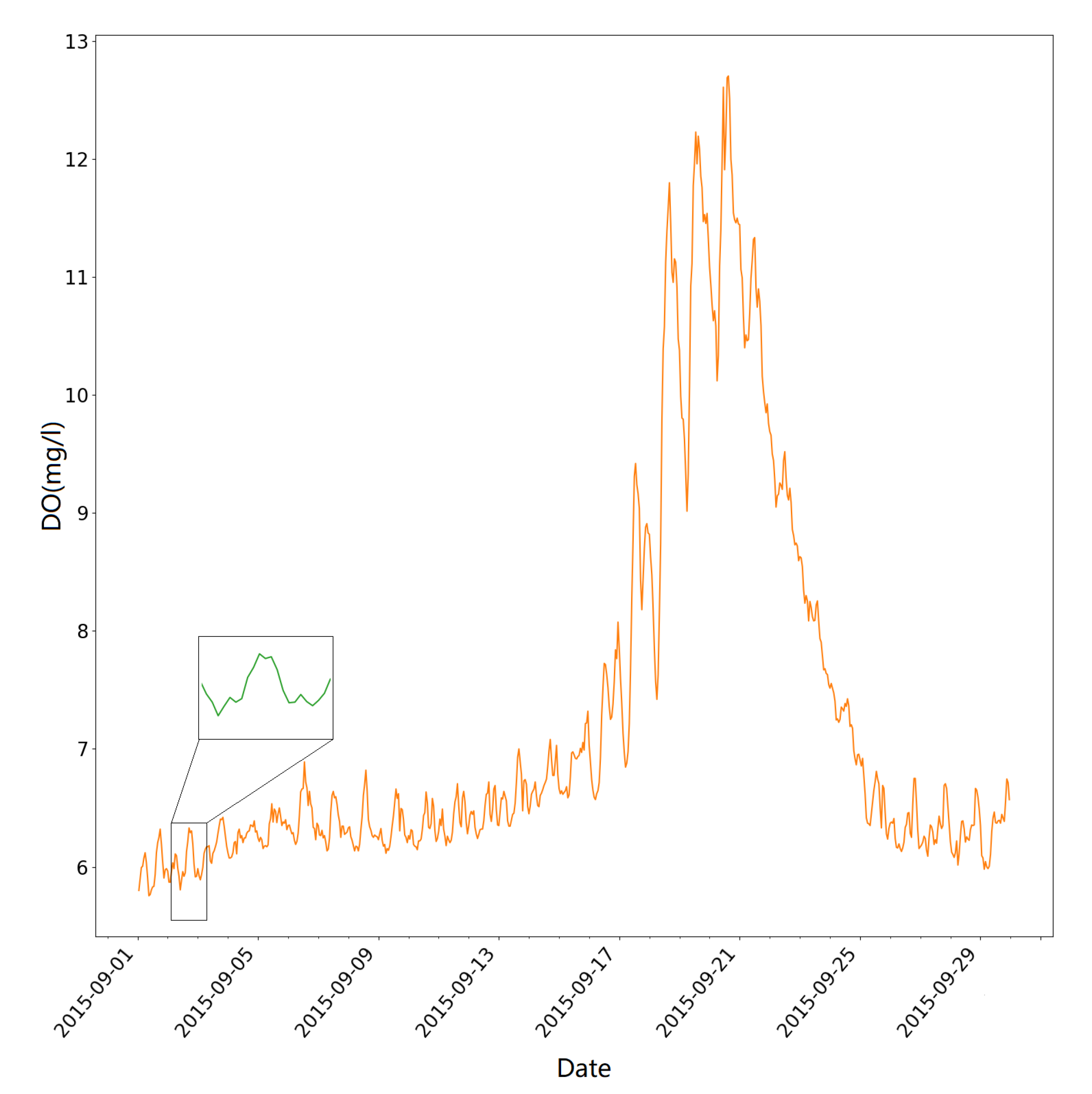
Figure 3 illustrates the changing patterns of DO both within a day and over a consecutive number of days. It is obvious that the concentration of DO follows a similar daily pattern, which makes it possible to predict the changing of DO. However, when tracking the concentration of DO in a larger time scale, it is plain to see that the mean value of the concentration of DO is increasing incrementally in the first half of the month and reach the peak value around 21 September. After keeping the high-level concentration for a few days, the DO level decreases gradually till the end of the month. This situation happens when unexpected activities are happening, such as heavy rainfall, excessive algae, and phytoplankton growth. In these circumstances, the predictive models should capture the daily temporal pattern when forecasting future DO concentration. Moreover, the model should be robust so it can have stable prediction performance at different time steps.
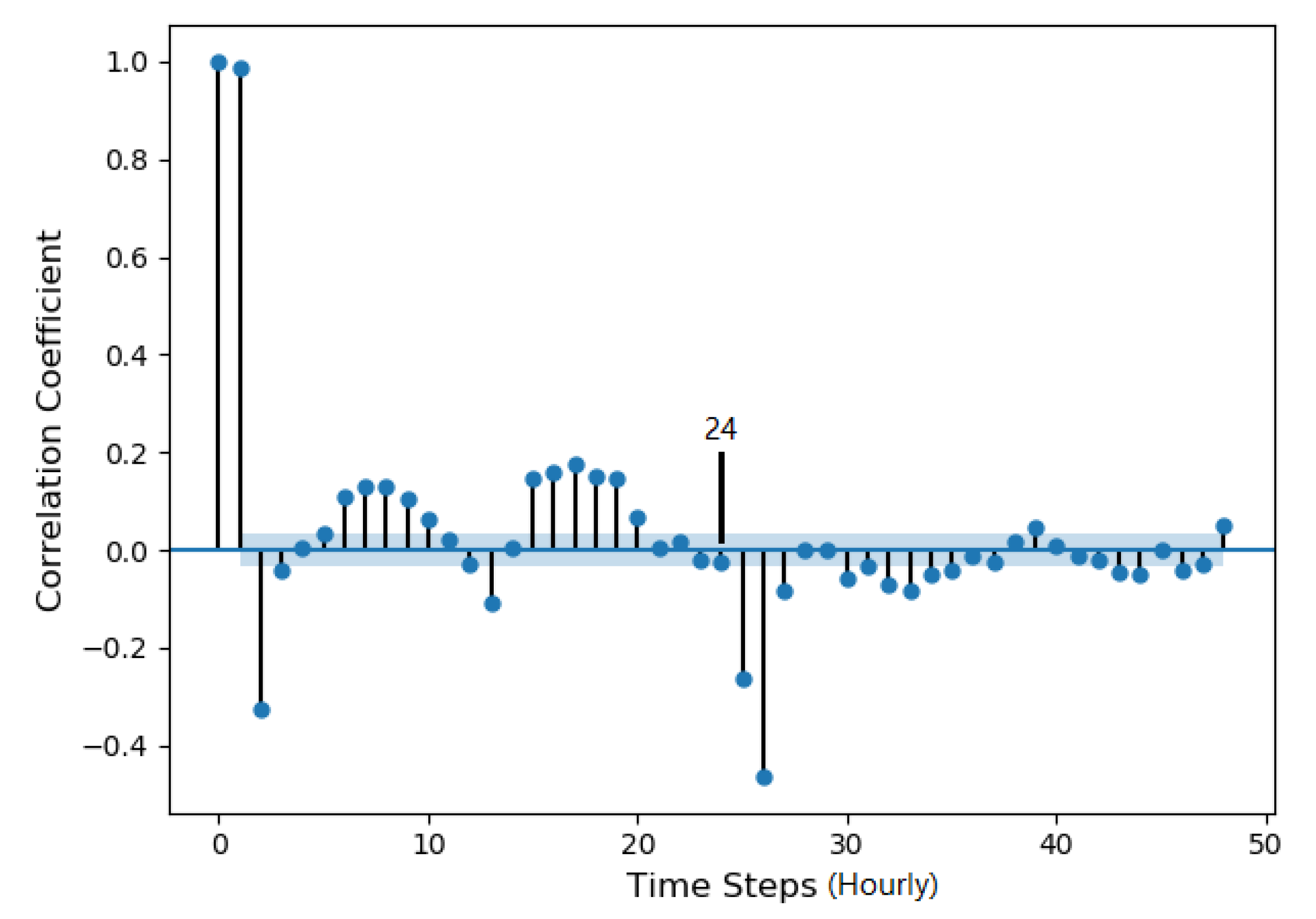
Figure 4 depicts the autocorrelation of DO for 48 hourly time steps over two days. The plot shows the correlation after the 26th lag is not statistical significance. It means that, in order to predict the trend of DO concentration, the information in the previous 26 h is the most important. This result is also supported by the fact that the concentration of DO follows a daily pattern (Figure 3).
Hence, by both considering the partial autocorrelation results and the trends of DO under different time scales, we choose to use the data from 24 historical time steps as the input for our predictive model. In this way, the input can cover the information from the previous 24 h, which indicates the complete daily pattern of the DO concentration.
2.2. kPCA-RNN Model Description
2.2.1. Kernel PCA Based Input Abstraction
Principal component analysis (PCA) is routinely applied for linear dimensionality reduction and feature abstraction [23]. The diagonal of the correlation matrix transforms the original principal correlated variables into principal uncorrelated (orthogonal) variables called principal components (PCs), which are weighed as linear combinations of the original variables. The eigenvalues of the PCs are a measure of associated variances, and the sum of the eigenvalues coincides with the total number of variables.
The standard PCA only allows linear dimensionality reduction. However, the multivariate water quality data have a more complicated structure which cannot be easily represented in a linear subspace. In this paper, kernel PCA (kPCA) [24] is chosen as a nonlinear extension of PCA to implement nonlinear dimensionality reduction for water quality variables. The kernel represents an implicit mapping of the data to a higher dimensional space where linear PCA is performed.
The PCA problem in feature space can be formulated as the diagonalization of an l-sample estimate of the covariance matrix [25], which can be defined as Equation (1):
where are centred nonlinear mappings of input variables . Then, we need to solve the following eigenvalue problem:
Note that all the solutions with lie in the span of . An equivalently problem is defined below:
where denotes the column vector such that , and K is a kernel matrix which satisfies the following conditions:
where Then, we can compute the kth nonlinear principal component of x as the projection of onto the eigenvector :
Then, the first nonlinear components are chosen, which have the desired percentage of data variance. By doing this, the complexity of the original data series can be greatly reduced.
2.2.2. Recurrent Neural Network
Recurrent Neural Networks (RNN) have gained tremendous popularity over the last few years because of their capability in handling unstructured sequential data. In contradistinction to the feed-forward neural network, RNN has the information travelling in both directions. Computations derived from the earlier input are fed back into the network, which is critical in learning the nonlinear relationships between multiple water quality variables.
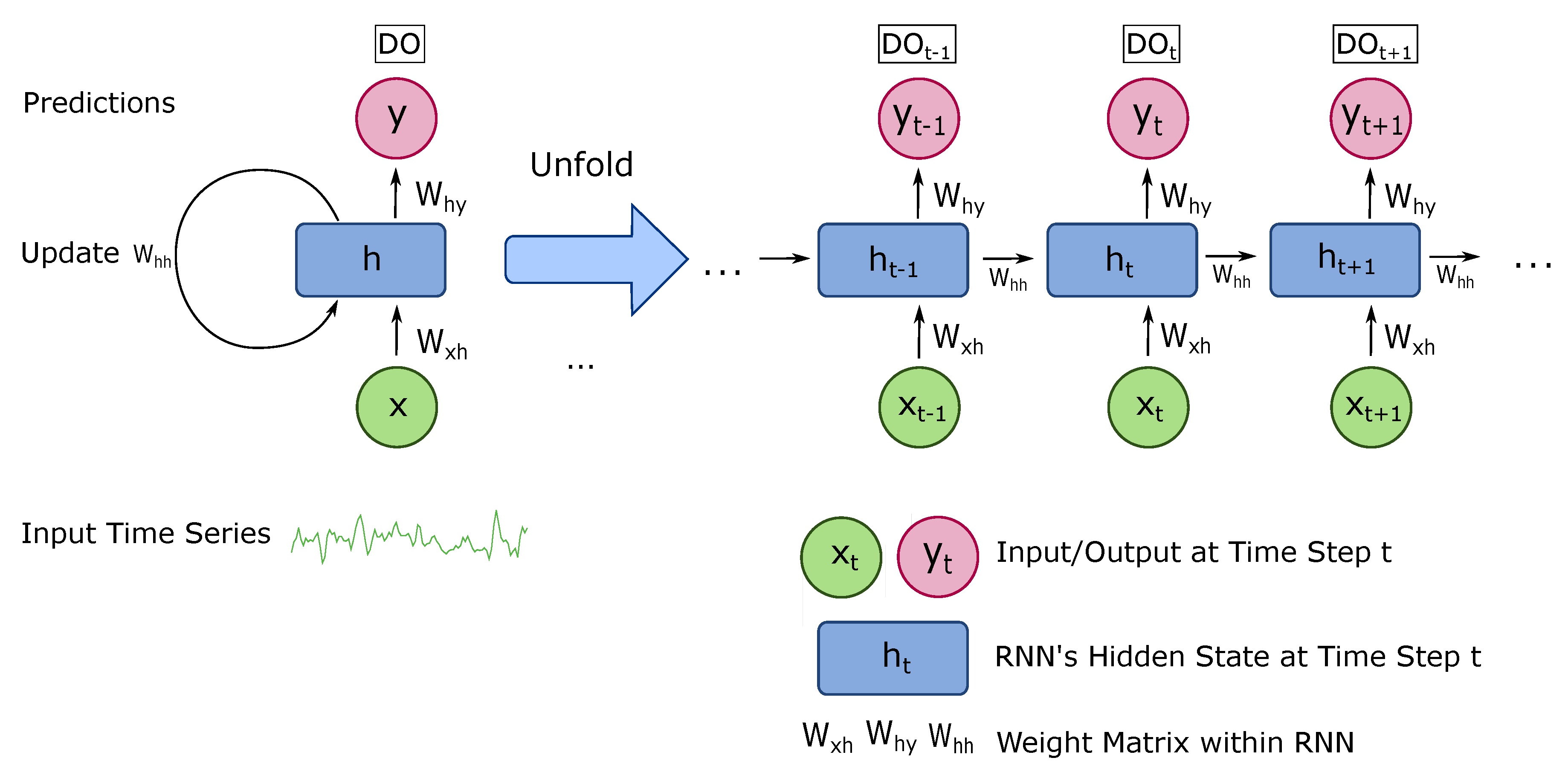
The general input to an RNN model is a variable-length sequence where and d represents the dimention of . At each time step, RNN maintains its internal hidden state h, which results in a hidden sequence of . The operation of an RNN at time step t can be formulated as:
where is an activation function, is the matrix of conventional weights between an input layer x and a hidden layer h, and is the matrix between a hidden layer h and itself at adjacent time steps.
The output of RNN is computed by:
where is the matrix of weights between the hidden layer h and output y.
As exhibited in Figure 5, the structure of the RNN model across time can be expressed as a deep neural network with one layer per time step. Because this feedback loop occurs at every time step in the series, each hidden state contains traces not only of the previously hidden state, but also of all those that preceded for as long as memory can persist.
Compared to the transitional feed-forward neural network, the recurrent structure in RNN can preserve the sequential information in its hidden state. In this approach, the input information can be spanned many time steps as it cascades forward to affect the processing of each new example. The features of RNN networks are especially suitable for processing time series water quality data because of the following reasons: Firstly, water quality data are periodically collected from different sensors and the previous values have strong relationship with the following changing. Secondly, the pattern of many water quality variables can only be recognized when enough historical data are involved and analysed.
In the proposed water quality predictive model, we apply the RNN structure with the LSTM cell [26]. To predict the concentration of DO at time step , the input time series include data in previous m time steps. Additionally, each time step has n water quality variables. Consequently, each input of the RNN model can be interpreted as a matrix. The explicit hyperparameters of our RNN model will be outlined in the following Section 3.2.
2.3. Model Evaluation
We compared the kPCA-RNN model with the following three machine learning methods:
- Feed-forward neural network (FFNN). FFNN has been broadly adopted for water quality analysis due to its capability in capturing nonlinear relationships within the short-term period [13].
- Support vector regression (SVR). SVR is a classic machine learning technique which can map inputs into higher dimensional space and interpret the problem as a linear regression [29].
The following performance indicators were applied to evaluate the predictive results. Those are the mean absolute error (MAE), the coefficient of determination (), the root mean square error (RMSE), and the percent of prediction within a factor of 1.1 (FA1.1) [30]:
where , , n, and m represent the observed value, the predicted value, the number of observations, and the number of predictions within a factor of 1.1 of the observed values, respectively. Additionally, .
2.4. Workflow of Predicting DO
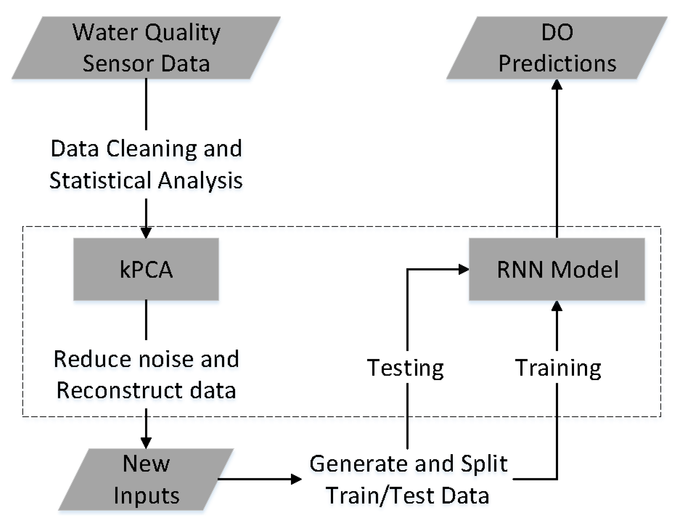
Figure 6 depicts the workflow of predicting the concentration of DO by using the kPCA-RNN model. There are two key steps in this workflow: applying the kPCA to denoise and reconstruct input data and implementing the RNN model to forecast the trend of dissolved oxygen in future time steps.
Firstly, the kPCA method is implemented on the tabulated water quality data (Table 1) to create corresponding principal components. The principal components with less importance are dropped to reduce the background noise in the original water quality dataset. Consequently, the remaining principal components are selected as new inputs for the predictive model.
Next, the input data are formed to matrix as we explained in Section 2.2.2. After training and testing the RNN model, the concentration of DO in the upcoming time steps can be estimated.
The kPCA-RNN model described in Figure 6 differs from most existing DO forecasting models in the following aspects:
- Instead of using the sensor data directly, the kPCA method is implemented to the water quality sensor data to construct new inputs based on principal components. This step can help reduce the background noise and keep the most useful information for DO forecasting tasks.
- The recurrent neural network is applied to process the time series water quality data. The recurrent structure offers a powerful way of capturing the temporal patterns across a period of time, which is critical in forecasting the changing of DO concentration in the future.
3. Model Application
3.1. Applying kPCA on the Water Quality Data
We applied the kPCA method to the water quality dataset (Table 1) and obtained five principal components (Table 2).
Five principal components (Table 2) are ordered by their corresponded eigenvalue. The first principal component is the linear combination of all the variables that have a maximum variance, so it accounts for as much variation in the data as possible. After that, each succeeding component, in turn, has the highest variance possible under the constraint that it is orthogonal to the preceding components. The cumulative variance proportion of the first four principal components is 94.8%. This indicates that, retaining only the first four principal components, one can explain 94.8% of the full variance.
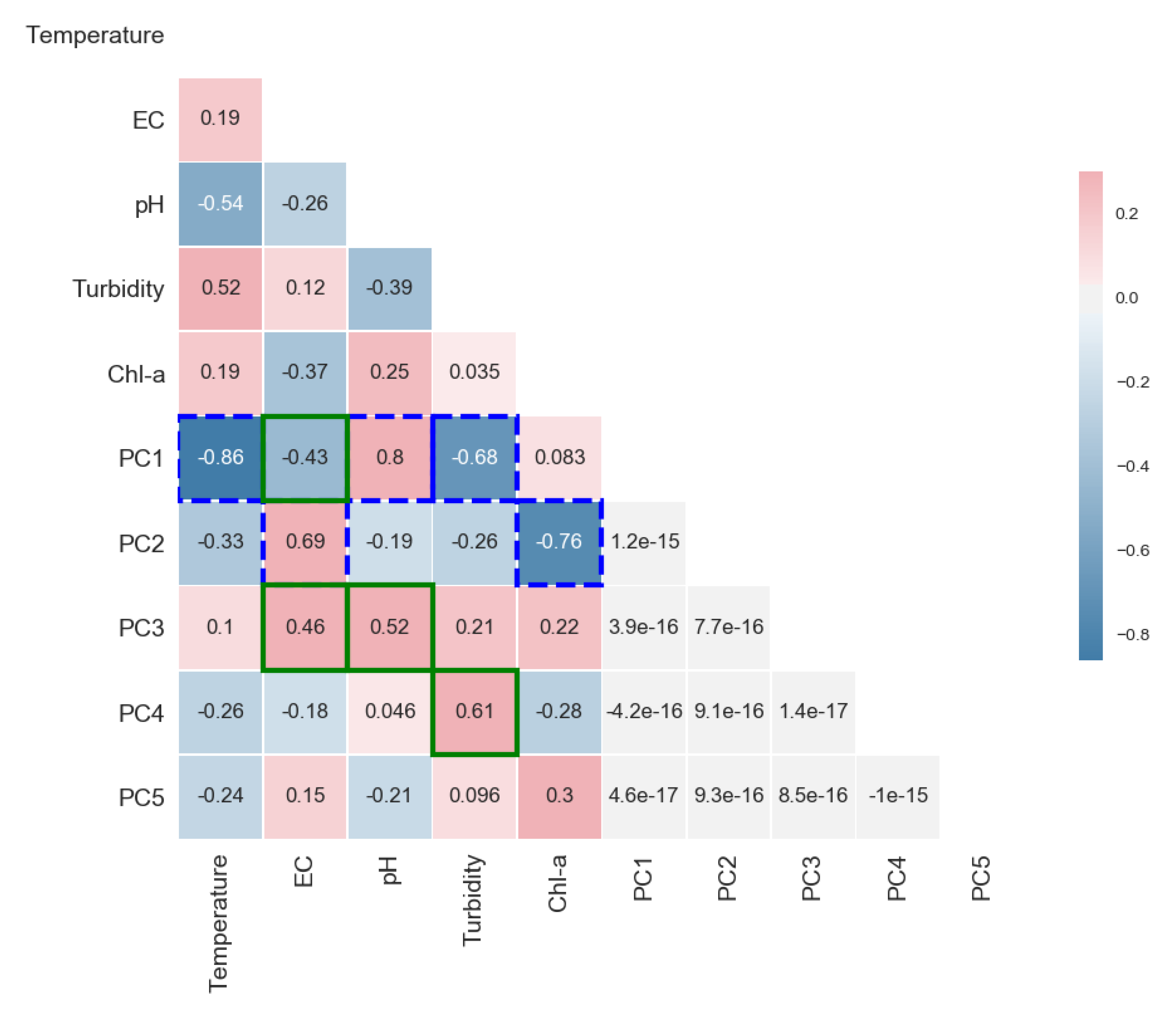
Figure 7 demonstrates the correlation scores between each water quality variable and a principal component (PC). The value at each cross point represents the correlation between two different items which are named on the left and bottom of the figure. This figure shows how each water quality variable contributes to each PC and also gives one the insight into how each PC can represent the information contained in different water quality variables.
As has been pointed out, the first principal component (PC1) has the highest correlation (dotted box, Figure 7) with variables like temperature, pH and turbidity. The three dotted boxes in line 5 (PC1) highlight the highest correlation scores one got from the corresponding water quality variables (listed in the bottom axis). Furthermore, the second principal component (PC2) has the highest correlation (dotted box in line 6) with the remaining variables EC and Chl-a. This indicates that, by utilizing only principal components PC1 and PC2, most information involved in those five water quality variables can be presented. Furthermore, PC3 and PC4 also have a strong correlation with EC, pH, and Turbidity (solid box). On the contrary, PC5 has a low value of correlation coefficient to all water quality variables, which means it carries much noise information [31]. Accordingly, we accept the first four principal components as new inputs. The kPCA method can reduce the input size by 20% while still keeping the most valuable information.
3.2. RNN Hyperparameters Settings
One challenge of building a neural network model is optimizing the hyperparameters for predictive accuracy [32]. Generally, different neural network settings are required to achieve the promising results for different forecasting tasks. Hence, we need to choose proper neural network parameters for forecasting DO concentration in three different predictive horizons.
Three RNN models were designed to predict the next one, two, and three hours of DO concentration independently. Each RNN model has various parameters and they all accept four months of data (2928 samples) for training and one month of data (744 samples) for testing. Based on the partial autocorrelation analysis in Section 2.1.2, data from the previous 24 time steps were accepted as the model’s input when predicting the concentration of DO in each future step.
The hyperparameters of the three RNN models were defined in Table 3.
3.3. Results and Discussion
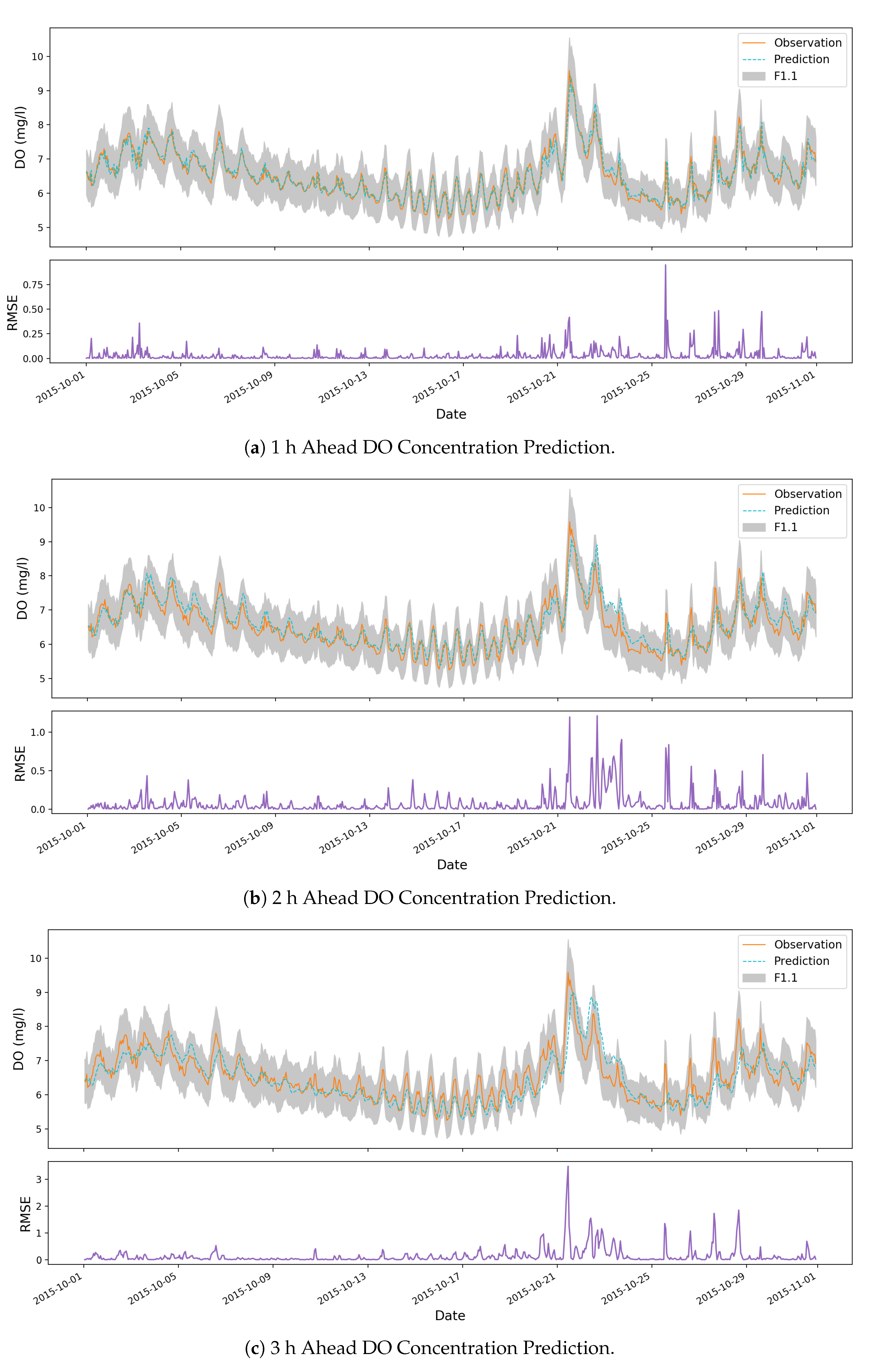
Figure 8 illustrates the forecasting of DO concentration during October 2015 under three different predictive horizons. The upper part of each subfigure compares the actual measurements and predictions of the DO concentration at each time index. In all the three subfigures, over 90% of the predictions are located in the F1.1 range. This means that the proposed kPCA-RNN model can capture the moving average of the DO concentration. By learning information from the previous 24 time steps, the model can avoid most of the severe bias estimations.
The model yields predictions with value of 0.908 for 1 h ahead forecasting in Figure 8. For 1 h ahead prediction, there is no time gap between the model’s inputs and the prediction. In order to predict DO concentration at a specific time step, the model can learn all the historical measurements until the previous hour. Thus, the proposed kPCA-RNN reaches the highest accuracy for 1 h ahead forecasting.
Similarly, our proposed model achieves value of 0.823 for 2 h ahead forecasting in Figure 8. When increasing the predictive horizon, the model does not predict what will happen after the last true measurement. Instead, the model needs to take a further step to generate the prediction. This usually happens when the model acts as an early warning system so there can be enough time for delivering management activities based on the forecasting results. In this circumstance, the model can only utilize what has been measured already to make the prediction. Hence, the prediction accuracy decreases slightly in this case.
In Figure 8, the model obtains value of 0.671 for 3 h ahead forecasting. As we discussed above, it becomes more challenging when one increases the predictive horizon, while, in this case, around 93% prediction results are still within ± 10% range of the original observations (FA1.1). This gives us confidence that the proposed kPCA-RNN model can still yield promising estimations. As we discussed in Section 1, the rapidly changing of DO concentration in a few hours can put aquatic life under high stress. Hence, the promising predictions in a few hours ahead are significant in early warning and changing management activities.
In addition, we also listed the RMSE value at each time step for all the three experimental cases (lower part of each subfigure in Figure 8). This offers us a detailed insight into the prediction performance of the proposed kPCA-RNN model. The RMSE figures clearly indicate that our model has a stable performance accuracy at most of the time steps. This is critical in applying the model in processing the real-world water quality sensor data.
As can be seen, most biased estimations happened between 21 October 2015 and 29 October 2015, where there was a strong fluctuation of DO concentration. In the water monitoring reports published by the Queensland Government, there was a large amount of discharge for total nutrients, dissolved and particulate nutrients during that period of time. On the contrary, the discharge in the previous months was low. It indicates that the trend of concentration of DO was changing more frequently and heavily in October. However, the kPCA-RNN model is trained based on the concentration of DO obtained from historical months with regular DO change. Consequently, there are some predictions below the high points of the observations; for example, the predictions around 22 October 2015. Hence, it is necessary to involve extra water quality data to cover a longer time period.
We additionally compared the performance of the kPCA-RNN model with three models stated in Section 2.3. The same data set described in Section 2.1.1 was applied in all cases. For FFNN, we set the same neural network size as in the kPCA-RNN model. For GRNN, the standard deviation is set to 10 for the high dimensional inputs. For SVR, the Radial Basis Function kernel (RBF) is taken as the nonlinear kernel. The corresponding results are listed in Table 4.
The kPCA-RNN models offer the best performance in all three of the prediction cases (Table 4). For example, in the 1 h ahead prediction, 99.5% of the predictions are within the FA1.1 range, which demonstrates that the model has a stable accuracy for most predictions.
Specifically, the kPCA-RNN model has 8%, 17% and 40% improved performance on the RMSE than the FFNN in all three of the cases, respectively. Similarly, the kPCA-RNN model achieves 43%, 52% and 21% improved performance on the RMSE over the SVR. Compared to GRNN, our proposed model gains 41%, 29% and 12% performance improvement on the RMSE scores. The FFNN, SVR and GRNN are ineffective in predicting the changing of DO concentration with 2 or 3 h predictive horizon because their model structures are not designed to handle time series data and the temporal pattern cannot be efficiently captured.
Hence, the kPCA-RNN model can perform as an early warning predictor for DO in application areas such as aquaculture ponds. By providing the DO significant changing alarm, farmers can consider appropriate actions to maintain the DO on a suitable level for the health of the aquatic ecosystem.
4. Conclusions
To summarize, the kPCA-RNN model was able to successfully predict the trend of DO in the following 1 to 3 h. We evaluated our model based on water quality data from Burnett River, Australia and compared it with the FFNN, SVR and GRNN methods. The results demonstrate that our method is more accurate and stable to the alternative methods, especially when the predictive horizon is increasing. Furthermore, as a data-driven modeling method, the kPCA-RNN model is not limited to a specific hydrological area and can be extended to predict various water quality variables.
For future work, inputs can be improved to include extra information such as rail fall and cover more extended periods of time. In addition, the water quality predictive model can be extended to support predicting multiple water variables simultaneously.
Author Contributions
Methodology, writing—original draft preparation, Y.-F.Z.; writing—review and editing, P.F.; project administration, writing—review and editing, P.J.T. All authors have read and agreed to the published version of the manuscript.
Funding
This research received no external funding.
Acknowledgments
This work was conducted within the CSIRO Digiscape Future Science Platform.
Conflicts of Interest
The authors declare no conflict of interest.
References
- Barzegar, R.; Adamowski, J.; Moghaddam, A.A. Application of wavelet-artificial intelligence hybrid models for water quality prediction: A case study in Aji-Chay River, Iran. Stoch. Environ. Res. Risk Assess. 2016, 30, 1797–1819. [Google Scholar] [CrossRef]
- Hrachowitz, M.; Benettin, P.; van Breukelen, B.M.; Fovet, O.; Howden, N.J.; Ruiz, L.; van der Velde, Y.; Wade, A.J. Transit times-the link between hydrology and water quality at the catchment scale. Wiley Interdiscip. Rev. Water 2016, 3, 629–657. [Google Scholar] [CrossRef] [Green Version]
- Jin, T.; Cai, S.; Jiang, D.; Liu, J. A data-driven model for real-time water quality prediction and early warning by an integration method. Environ. Sci. Pollut. Res. 2019, 26, 30374–30385. [Google Scholar] [CrossRef] [PubMed]
- Tomić, A.Š.; Antanasijević, D.; Ristić, M.; Perić-Grujić, A.; Pocajt, V. A linear and nonlinear polynomial neural network modeling of dissolved oxygen content in surface water: Inter- and extrapolation performance with inputs’ significance analysis. Sci. Total. Environ. 2018, 610–611, 1038–1046. [Google Scholar] [CrossRef]
- King, A.J.; Tonkin, Z.; Lieshcke, J. Short-term effects of a prolonged blackwater event on aquatic fauna in the Murray River, Australia: Considerations for future events. Mar. Freshw. Res. 2012, 63, 576–586. [Google Scholar] [CrossRef]
- Zhang, Y.; Thorburn, P.J.; Fitch, P. Multi-Task Temporal Convolutional Network for Predicting Water Quality Sensor Data. In Proceedings of the 26th International Conference on Neural Information Processing (ICONIP2019), Sydney, Australia, 12–15 December 2019; Volume 1142, pp. 122–130. [Google Scholar]
- Hawkins, C.P.; Olson, J.R.; Hill, R.A. The reference condition: Predicting benchmarks for ecological and water-quality assessments. J. North Am. Benthol. Soc. 2010, 29, 312–343. [Google Scholar] [CrossRef] [Green Version]
- Marcomini, A.; Suter II, G.W.; Critto, A. Decision Support Systems for Risk-Based Management of Contaminated Sites; Springer Science & Business Media: New York, NY, USA, 2008; Volume 763. [Google Scholar]
- Chubarenko, I.; Tchepikova, I. Modelling of man-made contribution to salinity increase into the Vistula Lagoon (Baltic Sea). Ecol. Model. 2001, 138, 87–100. [Google Scholar] [CrossRef]
- Chapra, S.; Pelletier, G.; Tao, H. QUAL2K: A Modeling Framework for Simulating River and Stream Water Quality; Documentation and user manual; Tufts University: Medford, MA, USA, 2003. [Google Scholar]
- Ay, M.; Özgür, K. Estimation of dissolved oxygen by using neural networks and neuro fuzzy computing techniques. KSCE J. Civ. Eng. 2016, 21, 1631–1639. [Google Scholar] [CrossRef]
- Zhang, Y.; Thorburn, P.J.; Wei, X.; Fitch, P. SSIM -A Deep Learning Approach for Recovering Missing Time Series Sensor Data. IEEE Internet Things J. 2019, 6, 6618–6628. [Google Scholar] [CrossRef]
- Zhang, Y.; Fitch, P.; Vilas, M.P.; Thorburn, P.J. Applying Multi-Layer Artificial Neural Network and Mutual Information to the Prediction of Trends in Dissolved Oxygen. Front. Environ. Sci. 2019, 7, 46. [Google Scholar] [CrossRef]
- Antanasijević, D.; Pocajt, V.; Perić-Grujić, A.; Ristić, M. Modelling of dissolved oxygen in the Danube River using artificial neural networks and Monte Carlo Simulation uncertainty analysis. J. Hydrol. 2014, 519, 1895–1907. [Google Scholar] [CrossRef]
- Li, X.; Sha, J.; Wang, Z.l. A comparative study of multiple linear regression, artificial neural network and support vector machine for the prediction of dissolved oxygen. Hydrol. Res. 2017, 48, 1214–1225. [Google Scholar] [CrossRef]
- Sundermeyer, M.; Oparin, I.; Gauvain, J.L.; Freiberg, B.; Schlüter, R.; Ney, H. Comparison of feedforward and recurrent neural network language models. In Proceedings of the 2013 IEEE International Conference on Acoustics, Speech and Signal Processing, Vancouver, BC, Canada, 26–31 May 2013; pp. 8430–8434. [Google Scholar]
- Karami, J.; Alimohammadi, A.; Seifouri, T. Water quality analysis using a variable consistency dominance-based rough set approach. Comput. Environ. Urban Syst. 2014, 43, 25–33. [Google Scholar] [CrossRef]
- Liu, S.; Che, H.; Smith, K.; Chang, T. A real time method of contaminant classification using conventional water quality sensors. J. Environ. Manag. 2015, 154, 13–21. [Google Scholar] [CrossRef]
- Chuan Wang, W.; wing Chau, K.; Qiu, L.; bo Chen, Y. Improving forecasting accuracy of medium and long-term runoff using artificial neural network based on EEMD decomposition. Environ. Res. 2015, 139, 46–54. [Google Scholar] [CrossRef]
- Ambient Estuarine Water Quality Monitoring Data. Available online: https://data.qld.gov.au/dataset (accessed on 20 November 2017).
- Great Barrier Reef Catchment Loads Monitoring Program. Available online: https://www.reefplan.qld.gov.au/measuring-success/paddock-to-reef/catchment-loads/ (accessed on 1 June 2018).
- Macdonald, R.K.; Ridd, P.V.; Whinney, J.C.; Larcombe, P.; Neil, D.T. Towards environmental management of water turbidity within open coastal waters of the Great Barrier Reef. Mar. Pollut. Bull. 2013, 74, 82–94. [Google Scholar] [CrossRef]
- Wold, S.; Esbensen, K.; Geladi, P. Principal component analysis. Chemom. Intell. Lab. Syst. 1987, 2, 37–52. [Google Scholar] [CrossRef]
- Schölkopf, B.; Smola, A.; Müller, K.R. Kernel principal component analysis. In Proceeedings of the Artificial Neural Networks—ICANN’97: 7th International Conference; Lausanne, Switzerland, 8–10 October 1997, Springer Berlin Heidelberg: Berlin/Heidelberg, Germany, 1997; pp. 583–588. [Google Scholar]
- Ince, H.; Trafalis, T.B. Kernel principal component analysis and support vector machines for stock price prediction. IIE Trans. 2007, 39, 629–637. [Google Scholar] [CrossRef]
- Hochreiter, S.; Schmidhuber, J. Long short-term memory. Neural Comput. 1997, 9, 1735–1780. [Google Scholar] [CrossRef]
- Specht, D.F. A general regression neural network. IEEE Trans. Neural Netw. 1991, 2, 568–576. [Google Scholar] [CrossRef] [Green Version]
- Barzegar, R.; Moghaddam, A.A. Combining the advantages of neural networks using the concept of committee machine in the groundwater salinity prediction. Model. Earth Syst. Environ. 2016, 2, 26. [Google Scholar] [CrossRef] [Green Version]
- Granata, F.; Papirio, S.; Esposito, G.; Gargano, R.; de Marinis, G. Machine learning algorithms for the forecasting of wastewater quality indicators. Water 2017, 9, 105. [Google Scholar] [CrossRef] [Green Version]
- Roberts, W.; Williams, G.P.; Jackson, E.; Nelson, E.J.; Ames, D.P. Hydrostats: A Python package for characterizing errors between observed and predicted time series. Hydrology 2018, 5, 66. [Google Scholar] [CrossRef] [Green Version]
- Verbanck, M.; Josse, J.; Husson, F. Regularised PCA to denoise and visualise data. Stat. Comput. 2013, 25, 471–486. [Google Scholar] [CrossRef] [Green Version]
- Jaques, N.; Gu, S.; Turner, R.E.; Eck, D. Tuning recurrent neural networks with reinforcement learning. arXiv 2017, arXiv:1611.02796v3. [Google Scholar]
- Kingma, D.P.; Ba, J. Adam: A method for stochastic optimization. arXiv 2014, arXiv:1412.6980. [Google Scholar]
Figure 1.
Burnett River catchment area and the monitoring site. This monitoring site is part of the Queensland Government’s water quality monitoring network [21].Burnett River catchment area and the monitoring site.
Figure 1.
Burnett River catchment area and the monitoring site. This monitoring site is part of the Queensland Government’s water quality monitoring network [21].Burnett River catchment area and the monitoring site.

Figure 2.
Data distribution for six water quality variables.Data distribution for water quality variables.
Figure 2.
Data distribution for six water quality variables.Data distribution for water quality variables.

Figure 3.
The concentration of DO measured in October 2015. The orange line describes the overall trend of DO concentration in this month. The green shape is an example of the daily pattern of DO concentration.Temporal patterns of the DO concentration.
Figure 3.
The concentration of DO measured in October 2015. The orange line describes the overall trend of DO concentration in this month. The green shape is an example of the daily pattern of DO concentration.Temporal patterns of the DO concentration.

Figure 4.
Partial autocorrelation of DO. The concentration of DO is collected hourly.Partial autocorrelation of DO.
Figure 4.
Partial autocorrelation of DO. The concentration of DO is collected hourly.Partial autocorrelation of DO.

Figure 5.
Recurrent neural network for predicting DO.Recurrent neural network for predicting DO.

Figure 6.
Workflow for predicting DO by applying the kPCA-RNN model. The dotted box highlights the key components of this proposed workflow.Workflow for predicting DO by using the kPCA-RNN model.
Figure 6.
Workflow for predicting DO by applying the kPCA-RNN model. The dotted box highlights the key components of this proposed workflow.Workflow for predicting DO by using the kPCA-RNN model.

Figure 7.
Correlations between water quality variables and principal components.Correlations between water quality variables and principal Components.
Figure 7.
Correlations between water quality variables and principal components.Correlations between water quality variables and principal Components.

Figure 8.
1, 2 and 3 h ahead predicting for the concentration of DO. In the upper part of each subfigure, the grey shadow, solid line and dotted line represent the FA1.1 range, DO observations and predictions, respectively. The lower part of each subfigure describes the RMSE value at each time step.


Table 1.
Water quality data from 1 June 2015 to 31 October 2015.
| Variables | No. of Data | Unit | Min | Max | Median | Mean | SD 1 | CV 2 (%) |
|---|---|---|---|---|---|---|---|---|
| Temperature | 3672 | C | 16.1 | 27.9 | 21.0 | 21.4 | 2.3 | 11 |
| EC | 3672 | uS·cm | 613.0 | 49,150.0 | 45,750.0 | 44,712.1 | 3566.8 | 8 |
| pH | 3672 | 7.5 | 8.4 | 7.9 | 7.8 | 0.1 | 2 | |
| DO | 3672 | mg·L | 5.2 | 13.0 | 6.8 | 6.9 | 0.9 | 13 |
| Turbidity | 3672 | NTU | 2.6 | 63.0 | 8.2 | 9.5 | 4.7 | 50 |
| Chl-a | 3672 | g·L | 0.1 | 137.6 | 2.6 | 3.5 | 3.6 | 102 |
1 standard deviation; 2 coefficient of variation.
Table 2.
Descriptive statistics of five principal components.
| Principal Components | Eigenvalue | Cumulative Variance Proportion (%) |
|---|---|---|
| PC1 | 466.6 | 44.4 |
| PC2 | 285.3 | 71.5 |
| PC3 | 129.8 | 83.8 |
| PC4 | 114.8 | 94.8 |
| PC5 | 55.1 | 100.0 |
Table 3.
Experiments settings.
| Model Settings | Experimental Cases | ||
|---|---|---|---|
| 1 h Ahead | 2 h Ahead | 3 h Ahead | |
| No. of Hidden Layers | 1 | 2 | 3 |
| No. of Hidden Units | 40 | 30 | 20 |
| Recurrent Cell | LSTM 1 | LSTM 1 | LSTM 1 |
| Optimizer | Adam 2 | Adam 2 | Adam 2 |
| No. of Historical Time Steps | 24 | 24 | 24 |
| No. of Training Data | 2928 | 2928 | 2928 |
| No. of Testing Data | 744 | 744 | 744 |
Table 4.
Performance comparison with the FFNN, SVR and GRNN.
| Predictive Models | Evaluation Criteria | |||
|---|---|---|---|---|
| MAE | RMSE | FA1.1 | ||
| 1 h Ahead Prediction | ||||
| kPCA-RNN Model | 0.149 | 0.908 | 0.208 | 0.995 |
| FFNN | 0.175 | 0.893 | 0.224 | 0.989 |
| SVR | 0.219 | 0.810 | 0.299 | 0.962 |
| GRNN | 0.263 | 0.727 | 0.355 | 0.944 |
| 2 h Ahead Prediction | ||||
| kPCA-RNN Model | 0.211 | 0.823 | 0.288 | 0.973 |
| FFNN | 0.258 | 0.757 | 0.338 | 0.958 |
| SVR | 0.314 | 0.594 | 0.437 | 0.890 |
| GRNN | 0.295 | 0.648 | 0.403 | 0.926 |
| 3 h Ahead Prediction | ||||
| kPCA-RNN Model | 0.303 | 0.671 | 0.394 | 0.926 |
| FFNN | 0.455 | 0.358 | 0.550 | 0.756 |
| SVR | 0.358 | 0.515 | 0.478 | 0.858 |
| GRNN | 0.320 | 0.562 | 0.450 | 0.910 |
© 2020 by the authors. Licensee MDPI, Basel, Switzerland. This article is an open access article distributed under the terms and conditions of the Creative Commons Attribution (CC BY) license (http://creativecommons.org/licenses/by/4.0/).
Share and Cite
MDPI and ACS Style
Zhang, Y.-F.; Fitch, P.; Thorburn, P.J. Predicting the Trend of Dissolved Oxygen Based on the kPCA-RNN Model. Water 2020, 12, 585. https://doi.org/10.3390/w12020585
AMA Style
Zhang Y-F, Fitch P, Thorburn PJ. Predicting the Trend of Dissolved Oxygen Based on the kPCA-RNN Model. Water. 2020; 12(2):585. https://doi.org/10.3390/w12020585
Chicago/Turabian StyleZhang, Yi-Fan, Peter Fitch, and Peter J. Thorburn. 2020. "Predicting the Trend of Dissolved Oxygen Based on the kPCA-RNN Model" Water 12, no. 2: 585. https://doi.org/10.3390/w12020585
Note that from the first issue of 2016, this journal uses article numbers instead of page numbers. See further details here.