Assessment of Seasonal Changes in Water Chemistry of the Ridracoli Water Reservoir (Italy): Implications for Water Management

 , , , ,
Abstract
:1. Introduction
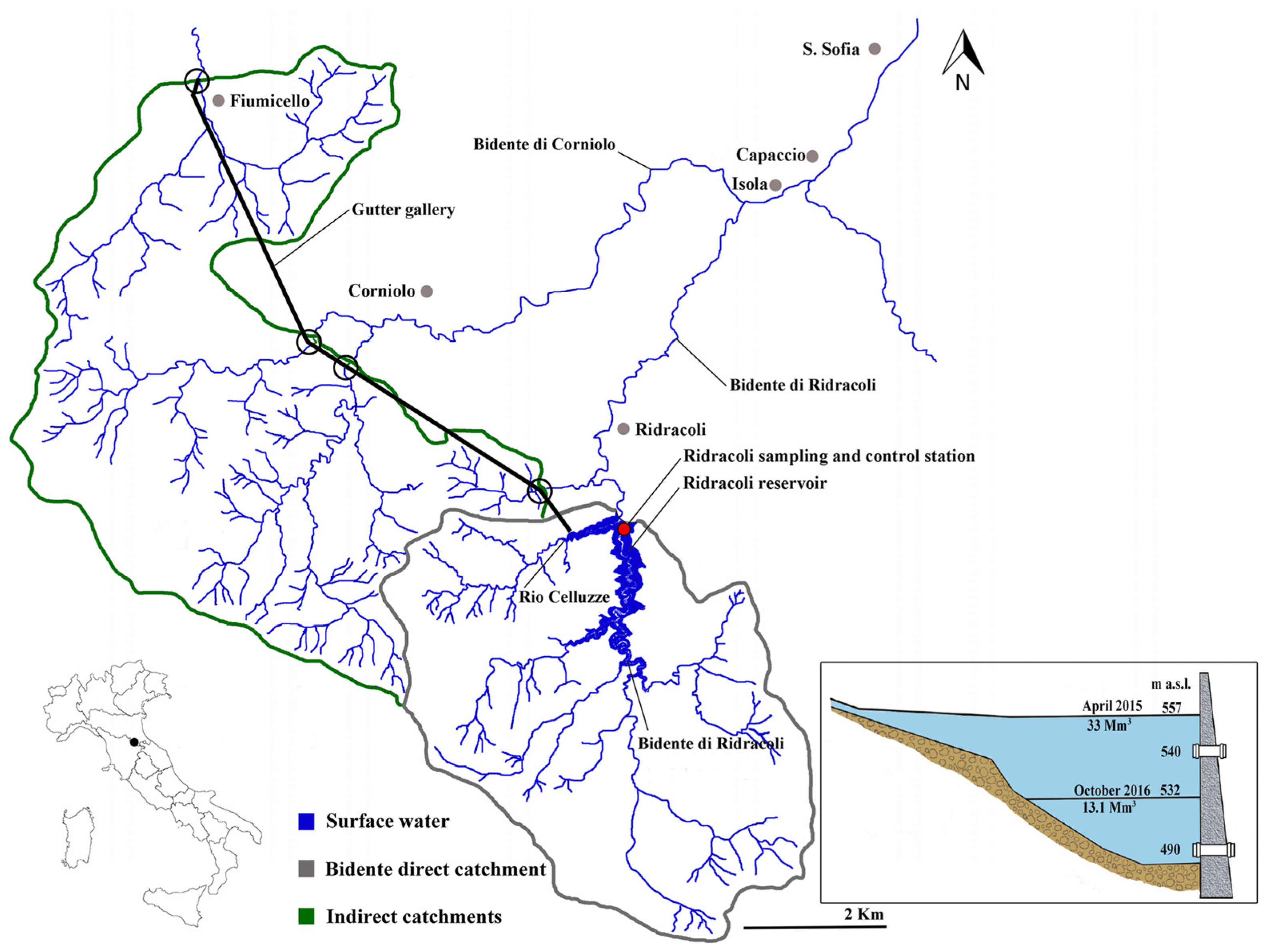
2. Study Area
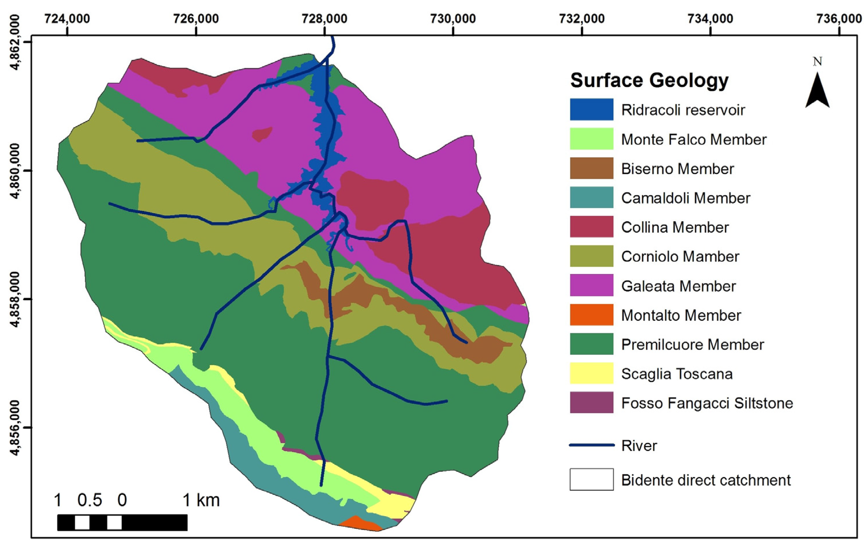
2.1. Geological Setting
2.2. Water Reservoir Management.
3. Methods
4. Results
4.1. Reservoir Volume and Water Level
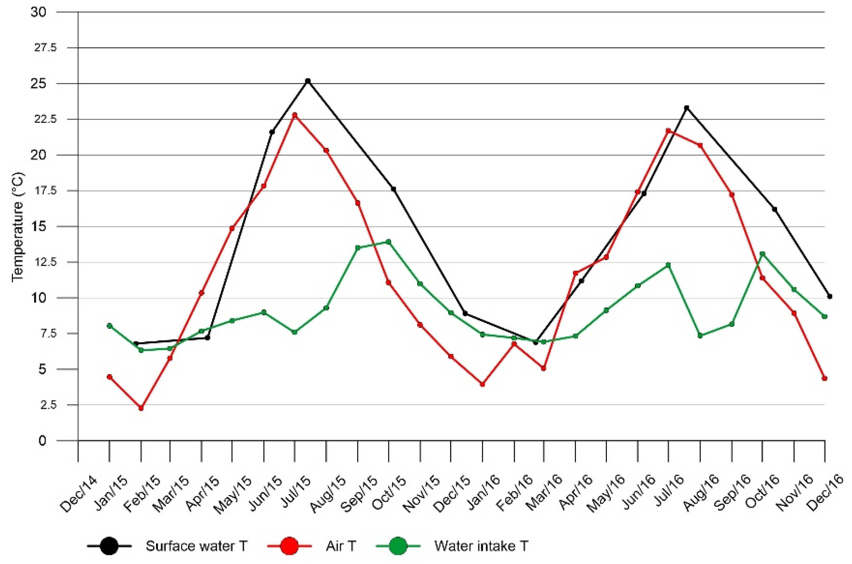
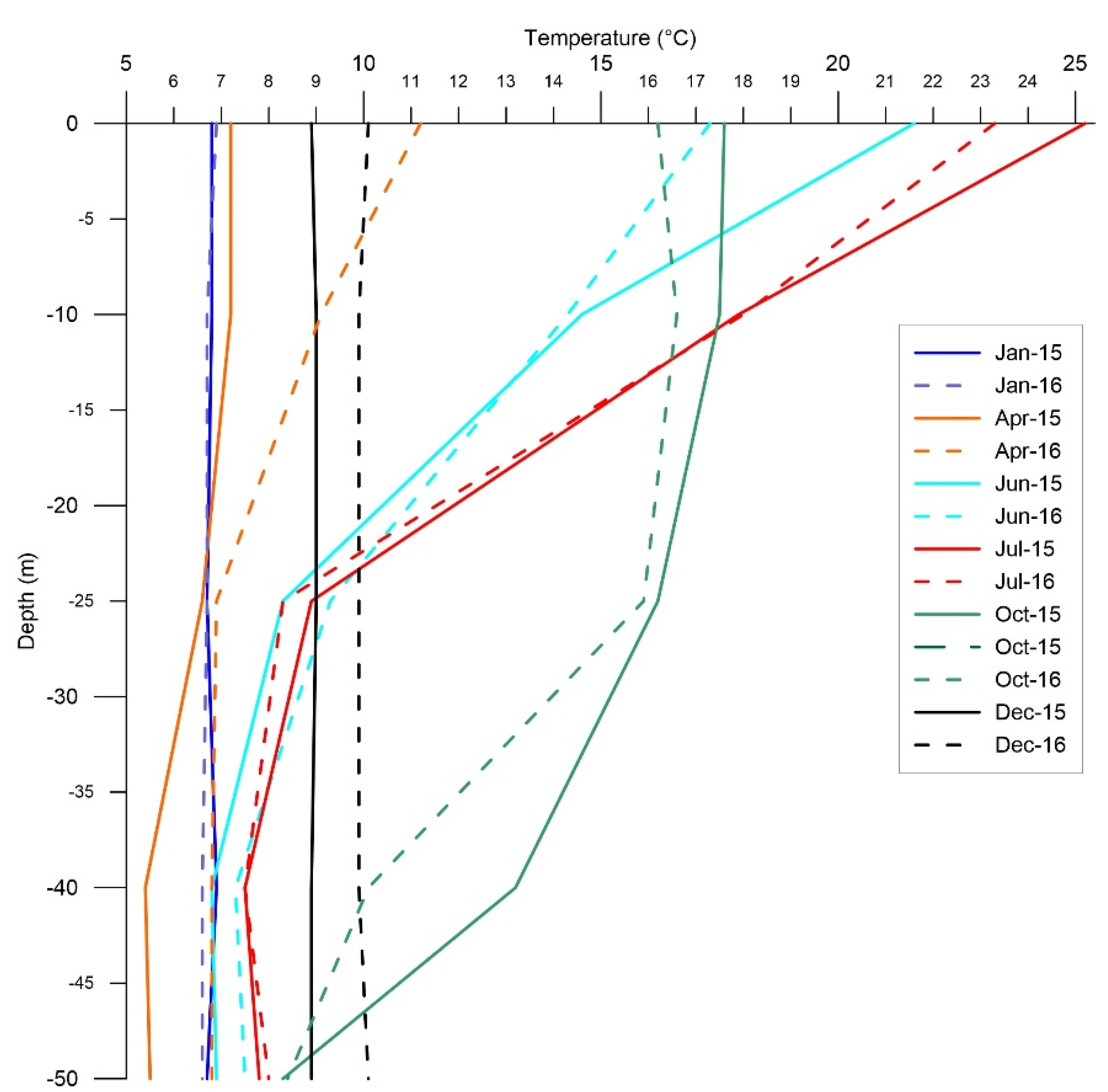
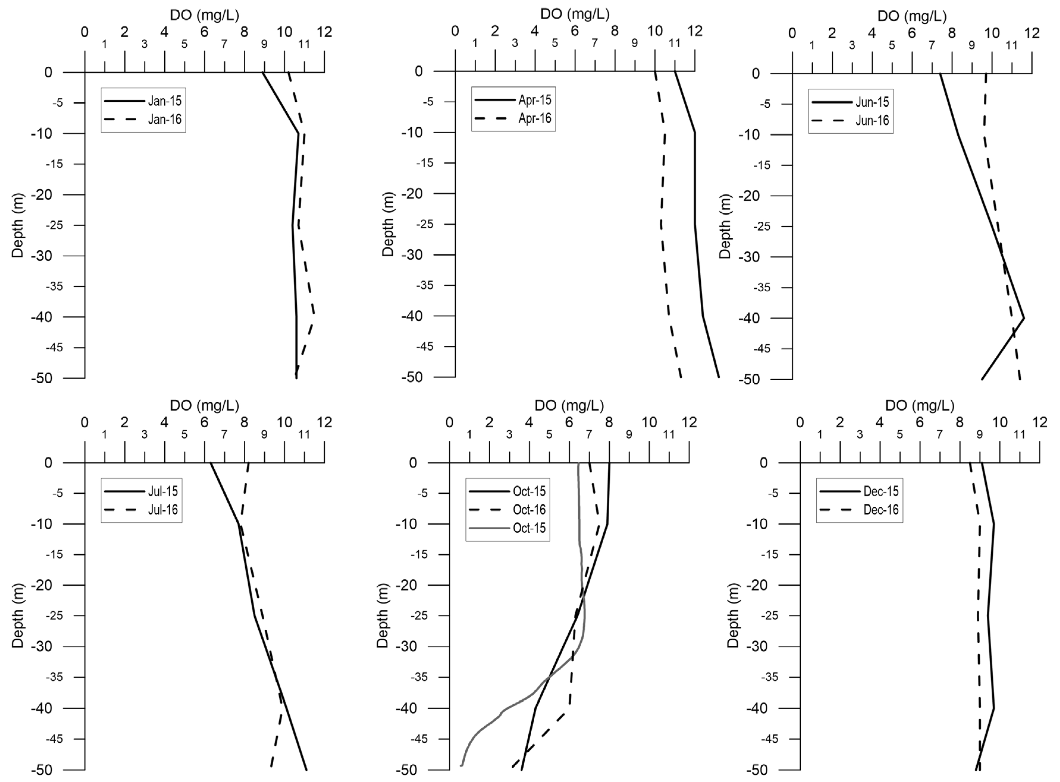
4.2. Physical Parameters
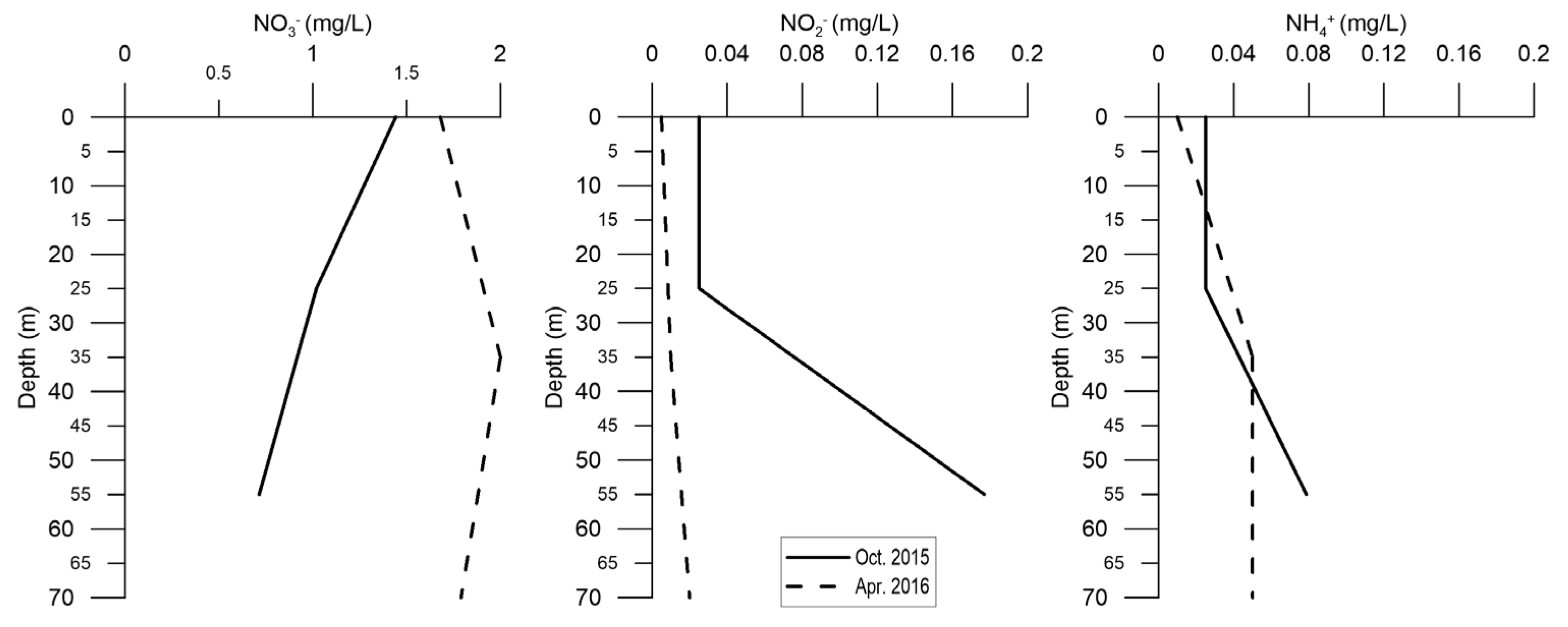
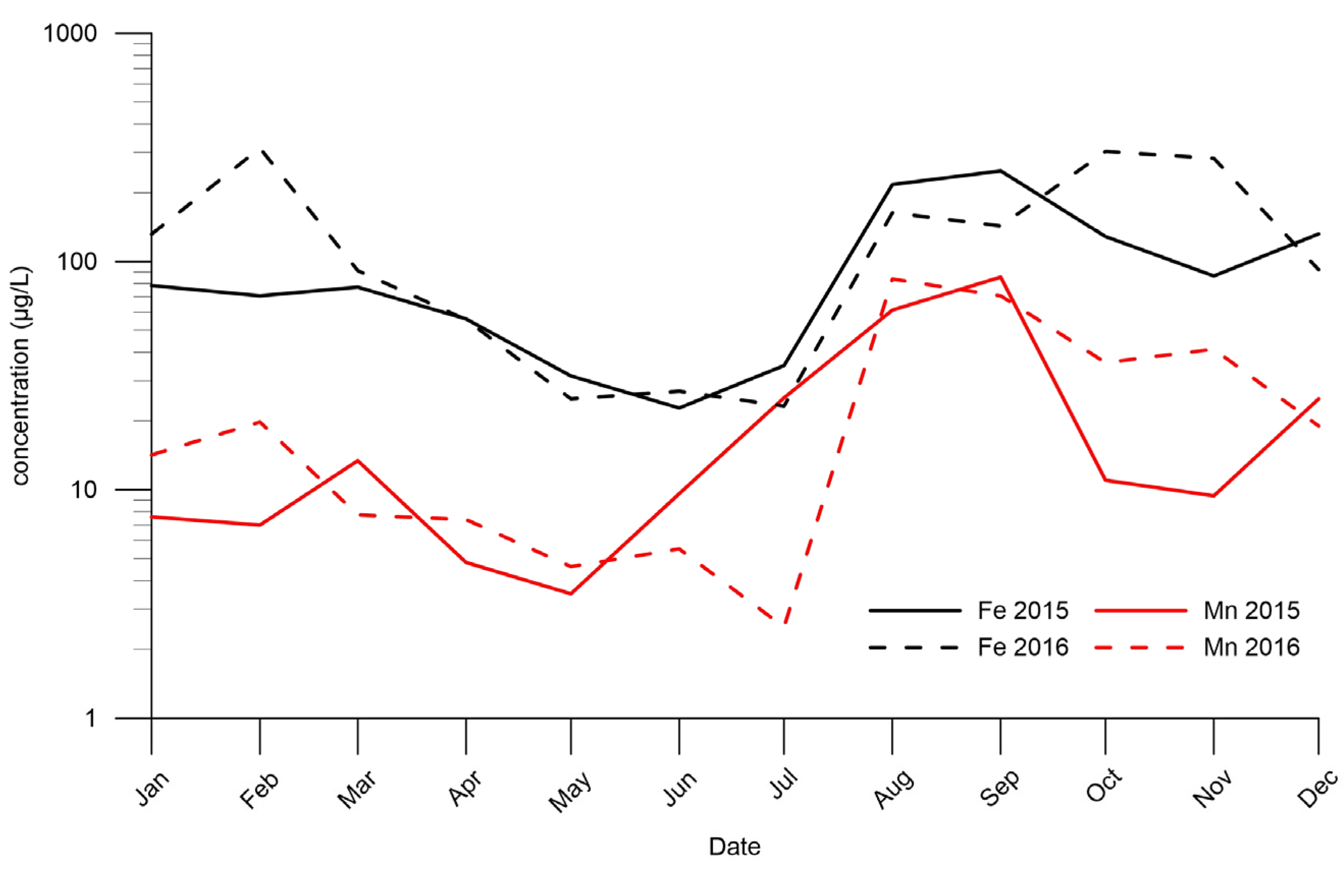
4.3. Chemical Parameters
5. Discussion
6. Conclusions
Supplementary Materials
Author Contributions
Funding
Acknowledgments
Conflicts of Interest
References
- Mailhot, A.; Talbot, G.; Ricard, S.; Turcotte, R.; Guinard, K. Assessing the potential impacts of dam operation on daily flow at ungauged river reaches. J. Hydrol. Regional Studies 2018, 18, 156–167. [Google Scholar] [CrossRef]
- Marcinkowski, P.; Grygoruk, M. Long-term downstream effects of a dam on a lowland river flow regime: Case study of the Upper Narew. Water 2017, 9, 783. [Google Scholar] [CrossRef] [Green Version]
- Magilligan, F.J.; Nislow, K.H. Changes in hydrologic regime by dams. Geomorphology 2005, 71, 61–78. [Google Scholar] [CrossRef]
- Schmutz, S.; Moog, O. Dams: Ecological impacts and management. In Riverine Ecosystem Management; Springer: Berlin/Heidelberg, Germany, 2018; pp. 111–127. [Google Scholar]
- Merritt, D.M.; Scott, M.L.; Poff, N.L.; Auble, G.T.; Lytle, D.A. Theory, methods and tools for determining environmental flows for riparian vegetation: Riparian vegetation-flow response guilds. Freshw. Biol. 2009, 55, 206–225. [Google Scholar] [CrossRef]
- Jansson, R. The effect of dams on biodiversity. In Dams under Debat; Johansson, B., Sellberg, B., Eds.; Swedish Research Council Formas: Stockholm, Sweden, 2006. [Google Scholar]
- Ampadu, B.; Akurugu, B.A.; Zango, M.S.; Abanyie, S.K. Assessing the impact of a dam on the livelihood of surrounding communities: A case study of Vea Dam in the Upper East Region of Ghana. J. Environ. Earth Sci. 2015, 5, 4. [Google Scholar]
- Pott, D.B. Dams and disease: Ecological design and health impacts on large dams, canals and irrigation systems. J. Hydraul. Eng. 2000, 126, 392. [Google Scholar] [CrossRef]
- Munyati, C. A spatial analysis of eutrophication in dam reservoir water on the Molopo River at Mafikeng, South Africa. Sustain. Water Qual. Ecol. 2015, 6, 31–39. [Google Scholar] [CrossRef]
- van Ginkel, C.E.; Silberbauer, M.J. Temporal trends in total phosphorus, temperature, oxygen, chlorophyll-a and phytoplankton populations in Hartbeespoort Dam and Roodeplaat Dam, South Africa, between 1980 and 2000. Afr. J. Aquat. Sci. 2007, 32, 63–70. [Google Scholar] [CrossRef]
- Ziaie, R.; Mohammadnezhad, B.; Taheriyoun, M.; Karimi, A.; Amiri, S. Evaluation of thermal stratification and eutrophication in Zayandeh Roud Dam Reservoir using two-dimensional CE-QUAL-W2 Model. J. Environ. Eng. 2019, 145, 05019001. [Google Scholar] [CrossRef]
- Mao, Y.; He, Q.; Li, H.; Su, X.; Ai, H. Thermal structure-induced biochemical parameterseters stratification in a subtropical dam reservoir. Water Environ. Res. 2018, 90, 2036–2048. [Google Scholar] [CrossRef]
- Hawkins, P.R. Thermal and chemical stratification and mixing in a small tropical reservoir, Solomon Dam, Australia. Freshw. Biol. 1985, 15, 493–503. [Google Scholar] [CrossRef]
- Lake, B.A.; Coolidge, K.M.; Norton, S.A.; Amirbahman, A. Factors contributing to the internal loading of phosphorus from anoxic sediments in six Maine, USA, lakes. Sci. Total Environ. 2007, 373, 534–541. [Google Scholar] [CrossRef] [PubMed]
- Chen, S.; Little, J.C.; Carey, C.C.; McClure, R.P.; Lofton, M.E.; Lei, C. Three-Dimensional effects of artificial mixing in a shallow drinking-water Resevoir. Water Environ. Res. 2018, 54, 425–441. [Google Scholar] [CrossRef]
- Munger, Z.W.; Carey, C.C.; Gerling, A.B.; Hamre, K.D.; Doubek, J.P.; Klepatzki, S.D.; McClure, R.P.; Schreiber, M.E. Effectiveness of hypolimnetic oxygenation for preventing accumulation of Fe and Mn in a drinking water reservoir. Water Res. 2016, 106, 1–14. [Google Scholar] [CrossRef] [PubMed]
- Morris, G.L.; Fan, J. Reservoir Sedimentation Handbook; McGraw-Hill Book Co.: New York, NY, USA, 1998. [Google Scholar]
- Arnason, J.G.; Fletcher, B.A. A 40+ year record of Cd, Hg, Pb, and U deposition in sediments of Patroon Reservoir, Albany Country, NY, USA. Environ. Pollut. 2003, 123, 383–391. [Google Scholar] [CrossRef]
- de Araújo, J.C.; Güntner, A.; Bronstert, A. Loss of reservoir volume by sediment deposition and its impact on water availability in semiarid Brazil. Hydrol. Sci. J. 2006, 51, 157–170. [Google Scholar] [CrossRef]
- Randle, T.J.; Bounty, J.A. Sediment Analysis Guidelines for Dam Removal; U.S. Department of the Interior, Bureau of Reclamation for the Federal Advisory Committee on Water Information, Subcommittee on Sedimentation: Denver, CO, USA, 2017.
- UNESCO Sediment Issues & Sediment Management in Large River Basins: Interim Case Study Synthesis Report; UNESCO Office in Beijing, International Research and Training Centre on Erosion and Sedimentation (China): Beijing, China, 2011; p. 82.
- Thompson, T.; Fawell, J.; Kunikane, S.; Jackson, D.; Appleyard, S.; Callan, P.; Bartram, J.; Kingston, P. Chemical Safety of Drinking-Water: Assessing Priorities for Risk Management; World Health Organization: Geneva, Switzerland, 2007; p. 160. [Google Scholar]
- Jørgensen, S.E.; Tundisi, J.G.; Tundisi, T.M. Handbook of Inland Aquatic Ecosystem Management; CRC Press: Boca Raton, FL, USA; Taylor & Francis Group: Abingdon-on-Thames, UK, 2013; p. 452. [Google Scholar]
- Calmano, W.; Hong, J.; Förstner, U. Binding and mobilization of heavy metals in contaminated sediments affected by pH and redox potential. Water Sci. 1993, 28, 223–235. [Google Scholar] [CrossRef] [Green Version]
- Buffi, G.; Manciola, P.; Grassi, S.; Barberini, M.; Gambi, A. Survey of the Ridracoli Dam, UAV-based photogrammetry and traditional topographic techniques in the inspection of vertical structures. Geomat. Nat. Hazards Risk 2017, 8, 1562–1579. [Google Scholar] [CrossRef] [Green Version]
- Buffi, G.; Manciola, P.; Grassi, S.; Barberini, M.; Gambi, A. Influence of Construction Joints in Arch-Gravity Dams Modelling: The Case of Ridracoli. In Proceedings of the 26th International Congress on Large Dams, Vienna, Austria, 4 July 2018; pp. 1047–1062. [Google Scholar]
- Uhlmann, D.; Paul, L.; Hupfer, M.; Fischer, R. Lakes and reservoirs. In Treatise on Water Science; Wilderer, P., Ed.; Elsevier: Amsterdam, The Netherlands, 2011; Volume 2, pp. 157–213. [Google Scholar]
- Arpae. Valutazione Dello Stato Delle Acque Superficiali Lacustri 2010–2013; Regional Agency for Prevention, Environmental and Energy, Emilia-Romagna Region: Emilia-Romagna, Italy, 2015; p. 47. [Google Scholar]
- Arpae. Valutazione Dello Stato Delle Acque Superficiali Lacustri 2014–2016; Regional Agency for Prevention, Environmental and Energy, Emilia-Romagna Region: Emilia-Romagna, Italy, 2018; p. 47. [Google Scholar]
- Ricci Lucchi, F. Turbidite dispersal in a Miocene deep-sea plain. Geol. Mijinbouw 1978, 57, 559–576. [Google Scholar]
- Gandolfi, G.; Paganelli, L.; Zufffa, G. Petrology and dispersal patterns in the Marnoso-arenacea formation (Miocene, Northern Apennines). J. Sediment. Petrol. 1983, 53, 493–507. [Google Scholar]
- Ricci Lucchi, F.; Valmori, E. Processi e meccanismi di sedimentazione. Sedimentologia 1980, 2, 212. (In Italian) [Google Scholar]
- Martelli, L.; Farabegoli, E.; Benini, A.; De Donatis, M.; Severi, P.; Pizziolo, M.; Pignone, R. La geologia del Foglio 265- S. Piero in Bagno. In La Cartografia Geologica della Emilia Romagna; Servizio Cartografico e Geologico, Regione Emilia Romagna: Bologna, Italy, 1994. [Google Scholar]
- Cornamusini, G.; Martelli, L.; Conti, P.; Pierucci, P.; Benini, A.; Bonciani, F.; Callegari, I.; Carmignani, L. Note Illustrative Della Carta Geologica d’Italia Alla Scala 1:50000, Foglio 266 Mercato Saraceno; ISPRA- Servizio Geologico d’Italia, Regione Emilia Romagna: Bologna, Italy, 2002. [Google Scholar]
- Benini, A.; Cremonini, G.; Martelli, L. Note Illustrative Della Carta Geologica d’Italia Alla Scala 1:50000, Foglio 255 Cesena; ISPRA-Servizio Geologico d’Italia: Rome, Italy, 2009. [Google Scholar]
- D.M.—Decree of the Ministry of Health. June 14 2017, Implementation of Directive (EU) 2015/1787, which amends Annexes II and III of Directive 98/83/EC on the quality of water intended for human consumption. In Amendment of Annexes II and III of Legislative Decree 2 February 2001; Gazzetta Ufficiale (G.U. n. 192 of the 18th of August 2017; Decree of the Ministry of Health: Rome, Italy, 2017. [Google Scholar]
- D. Lgs.—Legislative Decree. Lgs.—Legislative Decree. Implementation of Directive n. 80/777/EEC Relating to the Use and Marketing of Natural Mineral Waters; 25 January 1992, n. 105; Gazzetta Ufficiale (G.U. n. 39 of the 17th of February 1992); Gazzetta Ufficiale: Rome, Italy, 1992. [Google Scholar]
- UNI EN ISO 10304-1 Water Quality—Determination of Dissolved Anions by Liquid Chromatography of Ions—Part 1: Determination of Bromide, Chloride, Fluoride, Nitrate, Nitrite, Phosphate and Sulfate; ISO: Geneva, Switzerland, 2007.
- UNI EN ISO 10304-4 Water Quality—Determination of Dissolved Anions by Liquid Chromatography of Ions—Part 4: Determination of Chlorate, Chloride and Chlorite in Water with Low Contamination (ISO 10304-4:1997); ISO: Geneva, Switzerland, 1997.
- UNI EN ISO 17294-2. Water Quality—Application of Inductively Coupled Plasma Mass Spectrometry (ICP-MS)—Part 2: Determination of Selected Elements Including Uranium Isotopes; ISO: Geneva, Switzerland, 2016.
- D.Lgs.—Legislative Decree, 3 April 2006, n. 152. In Environmental Standards; Part III—Regulations on soil protection against desertification, protection of water from pollution and water resource management; Gazzetta Ufficiale (G-U.) n. 88 of the 14th of April 2006; Gazzetta Ufficiale: Rome, Italy, 2006.
- Pavan, V.; Romozeiu, R.; Cacciamani, C.; Di Lorenzo, M. Daily precipitation observations over Emilia-Romagna: Mean values and extremes. Int. J. Climatol. 2008, 28, 2065–2079. [Google Scholar] [CrossRef]
- Tomei, F.; Antolini, G.; Tomozeiu, R.; Pavan, V.; Villani, G.; Marletto, V. Analysis of Precipitation in Emilia-Romagna (Italy) and Impacts of Climate Change Scenarios. In Proceedings of the International Workshop Advances in Statistical Hydrology, Taormina, Italy, 23–25 May 2010. [Google Scholar]
- Rodriguez-Rodriguez, M.; Moreno-Ostos, E.; De Vicente, I.; Cruz-Pizarro, L.; Da Silva, S.L.R. Thermal structure and energy budget in a small high mountain lake: La Caldera, Sierra Nevada, Spain, New Zealand. J. Mar. Freshw. Res. 2004, 38, 879–894. [Google Scholar] [CrossRef]
- Wetzel, R.G.; Likens, G.E. The Heat Budget of Lakes. In Limnological Analyses; Springer: New York, NY, USA, 2000; pp. 45–56. [Google Scholar]
- Winton, R.S.; Calamita, E.; Wehrli, B. Reviews and syntheses: Dams, water quality and tropical reservoir stratification. Biogeosciences 2019, 16, 1657–1671. [Google Scholar] [CrossRef] [Green Version]
- Lewis, W.M., Jr.; McCutchan, J.H., Jr.; Roberson, J. Effects of Climatic Change on Temperature and Thermal Structure of a Mountain Reservoir. Water Resour. Res. 2019, 55, 1988–1999. [Google Scholar] [CrossRef]
- Langelier, W.F.; Ludwig, H.F. Graphical methods for indicating the mineral character of natural waters. AWWA 1942, 34, 335–352. [Google Scholar] [CrossRef]
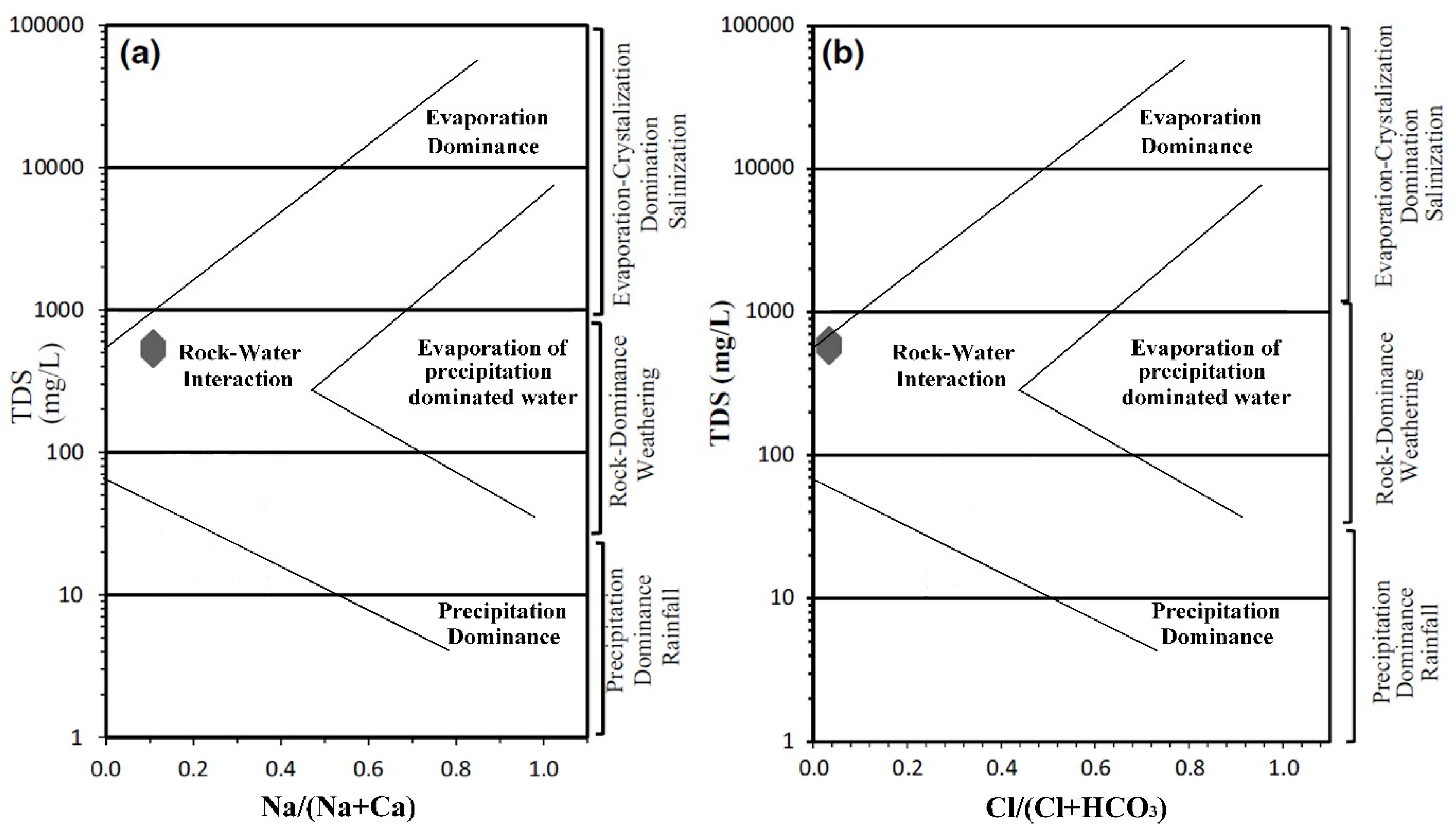
- Gibbs, R.J. Mechanisms controlling world water chemistry. Science 1970, 17, 1088–1090. [Google Scholar] [CrossRef]
- Dinelli, E.; Lucchini, F.; Mordenti, A.; Paganelli, L. Geochemistry of Oligocene-Miocene sandstones of the northern Apennines (Italy) and evolution of chemical features in relation to provenance changes. Sediment. Geol. 1999, 127, 193–207. [Google Scholar] [CrossRef]
- Lancianese, V.; Dinelli, E. Different spatial methods in regional geochemical mapping at high density sampling: An application on stream sediment of Romagna Apennines, Northern Italy. J. Geochem. Explor. 2015, 154, 143–155. [Google Scholar] [CrossRef]
- Magee, M.R.; Wu, C.H. Response of water temperatures and stratification to changing climate in three lakes with different morphometry. Hydrol. Earth Syst. Sci. 2017, 21, 6253–6274. [Google Scholar] [CrossRef] [Green Version]
- Burns, N.M. Using hypolimnetic dissolved oxygen depletion rates for monitoring lakes. N. Z. J. Mar. Freshw. 1995, 29, 1–11. [Google Scholar] [CrossRef]
- Berner, R.A. Early Diagenesis: A Theoretical Approach; Princeton University Press: Princeton, NJ, USA, 1980; p. 241. [Google Scholar]
- Jossette, G.; Leporcq, B.; Sanchez, N.; Philippon. Biogeochemical mass-balances (C, N, P, Si) in three large reservoirs of the Seine Basin (France). Biogeochemistry 1999, 47, 119–146. [Google Scholar] [CrossRef]
- Wall, L.G.; Tank, J.L.; Royer, T.V.; Bernot, M.J. Spatial and temporal variability in sediment denitrification within an agriculturally influenced reservoir. Biogeochemistry 2005, 76, 85–111. [Google Scholar] [CrossRef]
- Xiong, Z.; Guo, L.; Zhang, Q.; Liu, G.; Liu, W. Edaphic conditions regulate denitrification directly and indirectly by altering denitrifier abundance in wetlands along the Han River, China. Environ. Sci. Technol. 2017, 51, 5483–5491. [Google Scholar] [CrossRef]
- Sigg, L.; Sturm, M.; Kistler, D. Vertical transport of heavy metals by settling particles in Lake Zurich. Limnol. Oceanogr. 1987, 32, 112–130. [Google Scholar] [CrossRef] [Green Version]
- Balistrieri, L.S.; Murray, J.W.; Paul, B. The geochemical cycling of trace elements in a biogenic meromictic lake. Geochim. Cosmochim. Acta 1994, 58, 3993–4008. [Google Scholar] [CrossRef]
- Casamitjana, X.; Serra, T.; Colomer, J.; Baserba, C.; Perez-Losada, J. Effects of the water withdrawal in the stratification patterns of a reservoir. Hydrobiologia 2003, 504, 21–28. [Google Scholar] [CrossRef]
- Elci, S. Effects of thermal stratification and mixing on reservoir water quality. Limnology 2008, 9, 135–142. [Google Scholar] [CrossRef] [Green Version]
- D. Lgs. Legislative Decree, 2 February 2001, n. 31. In Implementation of Directive 98/83/EC on the Quality of Water Intended for Human Consumption as Amended and Supplemented by Legislative Decree February 2; Gazzetta Ufficiale (G.U.) n. 52 of the 3rd of March 2001; Gazzetta Ufficiale: Rome, Italy, 2002.
- Gibbs, M.; Kickey, C. Guidelines for Artificial Lakes. National Institute of Water & Atmospheric Research Ltd, Hamilton, New Zealand; Ministry of Building, Innovation and Employment. Available online: http://www.envirolink.govt.nz/assets/Envirolink/Guidelines-for-artificial-lakes.pdf (accessed on 24 January 2020).
- Singleton, V.L.; Little, J.C. Designing Hypolimnetic aeration and oxygenation systems—A review. Environ. Sci. Technol. 2006, 40, 7512–7520. [Google Scholar] [CrossRef]
- Nordin, R.N.; McKean, C.J.P. A Review of Lake Aeration as a Technique for Water Quality Improvement; APD Bulletin 22; British Columbia Ministry of Environment: Victoria, BC, Canada, 1982; p. 40. [Google Scholar]
- Phillips, P.; Bender, J.; Simms, R.; Rodriguez-Eaton, S.; Britt, C. Manganese removal from acid coal-mine drainage by a pond containing green algae and microbial mat. Water Sci. Technol. 1995, 31, 161–170. [Google Scholar] [CrossRef]
- Gantzer, A.; Bryant, L.D.; Little, J.C. Controlling soluble iron and manganese in a water-supply reservoir using hypolimnetic oxygenation. Water Res. 2009, 43, 1285–1294. [Google Scholar] [CrossRef] [PubMed]


| Member | % | Age | A/P (Lithology) | Formation |
|---|---|---|---|---|
| Monte Falco | 4.3 | Upper Oligocene | Pelite almost absent | Falterona Mount (FAL) |
| Biserno | 3.0 | Langhian-Serravallian | 0.2–0.33 | Marnoso-Arenacea (MAF) |
| Camaldoli | 3.2 | Upper Oligocene-Miocene | 2–10 | Falterona Mount (FAL) |
| Collina | 8.8 | Langhian-Serravallian | 0.2–0.33 | Marnoso-Arenacea (MAF) |
| Corniolo | 15.6 | Langhian-Serravallian | 0.33–0.5 | Marnoso-Arenacea (MAF) |
| Galeata | 18.7 | Langhian-Serravallian | 0.33–0.5 | Marnoso-Arenacea (MAF) |
| Montalto | 0.2 | Miocene | 0.33–2 | Falterona Mount (FAL) |
| Premilcuore | 41.9 | Langhian-Serravallian | 1–2 | Marnoso-Arenacea (MAF) |
| Scaglia Toscana | 1.3 | Upper Eocene-Lower Oligocene | Argillites, marly argillites and silty marls | Scaglia Toscana (STO) |
| Fosso Fangacci | 0.2 | Upper Oligocene-Lower Miocene | <1 | Siltstones of Fosso Fangacci (SFF) |
| Parameters | Average Reservoir | Surface Water (0 m) | Bottom Water (>−50) | Capaccio Water Treatment Plant | |||||||||||||
|---|---|---|---|---|---|---|---|---|---|---|---|---|---|---|---|---|---|
| Unit | Min | Median | Max | MAD | Min | Median | Max | MAD | Min | Median | Max | MAD | Min | Median | Max | MAD | |
| Hardness (CaCO3) | mg/L | 156.0 | 174.5 | 197.0 | 9.0 | 156.0 | 170.0 | 184.0 | 7.0 | 165.0 | 181.0 | 197.0 | 9.3 | 151.8 | 160.0 | 13.9 | 6.1 |
| T | °C | 5.4 | 8.7 | 25.2 | 4.7 | 6.8 | 13.7 | 25.2 | 6.7 | 5.5 | 7.7 | 10.1 | 1.2 | 6.3 | 8.6 | 13.9 | 2.3 |
| DO | mg/L | 3.0 | 9.7 | 13.2 | 2.1 | 6.3 | 8.7 | 11.0 | 1.4 | 3.0 | 10.0 | 13.2 | 3.1 | # | # | # | # |
| pH | 7.4 | 8.3 | 8.6 | 0.3 | 7.5 | 8.4 | 8.6 | 0.4 | 7.4 | 8.2 | 8.4 | 0.3 | 7.6 | 8.0 | 8.2 | 0.2 | |
| EC | µS/cm | 274.0 | 307.0 | 361.0 | 20.4 | 274.0 | 300.0 | 343.0 | 22.3 | 293.0 | 315.5 | 341.0 | 17.6 | # | # | # | # |
| TDS | mg/L | 380.7 | 417.9 | 463.9 | 19.3 | 381.4 | 408.1 | 441.9 | 15.7 | 403.0 | 433.3 | 463.9 | 19.2 | 372.5 | 392.0 | 427.4 | 13.1 |
| HCO3− | 178.9 | 212.9 | 240.3 | 12.0 | 180.6 | 207.0 | 224.5 | 10.5 | 201.3 | 219.6 | 240.3 | 10.6 | 185.1 | 195.2 | 215.0 | 7.4 | |
| SO42− | 20.0 | 23.0 | 25.0 | 1.4 | 21.0 | 23.6 | 25.0 | 1.5 | 20.0 | 22.9 | 25.0 | 1.4 | 19.6 | 22.6 | 25.3 | 1.3 | |
| Cl− | 4.0 | 5.0 | 6.7 | 0.8 | 4.0 | 5.0 | 6.3 | 0.7 | 4.0 | 5.1 | 6.7 | 0.8 | 4.0 | 5.4 | 6.3 | 0.8 | |
| Na+ | 5.0 | 6.0 | 8.0 | 0.9 | 5.0 | 6.0 | 8.0 | 0.9 | 5.0 | 5.9 | 7.0 | 0.8 | 5.3 | 5.7 | 7.0 | 0.5 | |
| Ca2+ | 46.6 | 56.0 | 62.1 | 4.0 | 46.6 | 54.1 | 61.0 | 4.3 | 53.7 | 60.0 | 62.1 | 2.8 | 51.0 | 55.6 | 59.8 | 2.4 | |
| Mg2+ | 8.6 | 10.9 | 12.0 | 1.0 | 9.0 | 10.7 | 12.0 | 1.1 | 9.6 | 10.9 | 12.0 | 0.9 | 10.0 | 10.6 | 11.5 | 0.4 | |
| K+ | 0.2 | 1.0 | 3.0 | 0.8 | 1.0 | 1.0 | 3.0 | 0.9 | 0.9 | 1.0 | 3.0 | 0.8 | 1.1 | 1.3 | 1.5 | 0.1 | |
| NO2− | <0.05 | <0.05 | 0.18 | n.a. | <0.01 | <0.05 | <0.05 | n.a. | 0.02 | 0.10 | 0.18 | n.a. | <0.01 | <0.01 | 0.04 | n.a. | |
| NO3− | 0.71 | 1.56 | 2.00 | 0.49 | 1.44 | 1.56 | 1.68 | 0.17 | 0.71 | 1.25 | 1.79 | 0.76 | 1.06 | 1.45 | 1.65 | 0.15 | |
| NH4+ | <0.05 | 0.05 | 0.08 | n.a. | <0.05 | <0.05 | <0.05 | n.a. | 0.05 | 0.06 | 0.08 | n.a. | <0.05 | <0.05 | <0.05 | n.a. | |
| Fe | µg/L | 7.5 | 16.1 | 55.3 | 17.4 | 7.5 | 31.4 | 55.3 | 33.8 | 12.6 | 16.1 | 19.6 | 4.9 | 22.8 | 88.8 | 313.6 | 92.1 |
| Mn | <1 | 2.4 | 329.0 | 131.5 | <1 | 18.5 | 36.0 | 24.7 | 1.1 | 165.1 | 329.0 | 231.9 | 2.5 | 12.2 | 85.4 | 25.8 | |
| Al | 4.5 | 14.2 | 62.6 | 22.3 | 6.8 | 14.1 | 21.4 | 10.3 | 4.5 | 33.6 | 62.6 | 41.1 | 24.8 | 105.8 | 339.3 | 86.1 | |
| Zn | 4.3 | 21.1 | 172.4 | 64.2 | 8.7 | 90.6 | 172.4 | 115.8 | 15.8 | 23.2 | 30.6 | 10.5 | # | # | # | # | |
© 2020 by the authors. Licensee MDPI, Basel, Switzerland. This article is an open access article distributed under the terms and conditions of the Creative Commons Attribution (CC BY) license (http://creativecommons.org/licenses/by/4.0/).
Share and Cite
Toller, S.; Giambastiani, B.M.S.; Greggio, N.; Antonellini, M.; Vasumini, I.; Dinelli, E. Assessment of Seasonal Changes in Water Chemistry of the Ridracoli Water Reservoir (Italy): Implications for Water Management. Water 2020, 12, 581. https://doi.org/10.3390/w12020581
Toller S, Giambastiani BMS, Greggio N, Antonellini M, Vasumini I, Dinelli E. Assessment of Seasonal Changes in Water Chemistry of the Ridracoli Water Reservoir (Italy): Implications for Water Management. Water. 2020; 12(2):581. https://doi.org/10.3390/w12020581
Chicago/Turabian StyleToller, Simone, Beatrice M. S. Giambastiani, Nicolas Greggio, Marco Antonellini, Ivo Vasumini, and Enrico Dinelli. 2020. "Assessment of Seasonal Changes in Water Chemistry of the Ridracoli Water Reservoir (Italy): Implications for Water Management" Water 12, no. 2: 581. https://doi.org/10.3390/w12020581