Uncertainty Analysis of a 1D River Hydraulic Model with Adaptive Calibration


1
Département de génie civil et de génie des eaux, Université Laval, Québec, QC G1V 0A6, Canada
2
Environnement et Changement Climatique Canada (ECCC), Québec, QC G1J 0C3, Canada
*
Author to whom correspondence should be addressed.
Water 2020, 12(2), 561; https://doi.org/10.3390/w12020561
Submission received: 15 January 2020
/
Revised: 11 February 2020
/
Accepted: 14 February 2020
/
Published: 18 February 2020
(This article belongs to the Section Hydraulics and Hydrodynamics)
Abstract
:Water level modeling is a critical component of flood warning systems. A high-quality forecast requires the development of a hydraulic model that reliably accounts for the main sources of uncertainty. In this paper, a 1D hydraulic model with adaptive flow-based calibration was developed. This calibration resulted in roughness-flow relationships that allow Manning coefficients to be updated as a function of river flow, to limit errors throughout the flood cycle. An uncertainty analysis is then conducted for independent events, considering as the main source of uncertainty the error in the estimated input flows (upstream and lateral), and in the calibrated roughness coefficients. A set of parameters is generated by Latin Hypercube Sampling (LHS) from the characterization of these errors to evaluate their propagation to the variables of interest, namely water level and flow. These are evaluated by performance metrics (scores) such as the reliability diagram and the continuous rank probability score (CRPS). The adaptive flow-based calibration considerably reduced the error of the 1D model and improved its performance over time and throughout the flood events. The uncertainty analysis resulted in consistent accuracy improvements over a deterministic simulation with gains of 20% to 32%, depending on the combined parameters. Good reliability is also reached for most stations, with resulting spreads and Root Mean Square Error (RMSE) close to one another. The proposed methodology has the potential to improve the descriptive capability of 1D river hydraulic models and to increase their reliability when included in forecasting systems.
1. Introduction
Hydraulic modeling is a key component of any water level forecasting system in rivers. A precise and reliable water level forecast helps prevent flood damage and properly plan interventions in the event of a high risk. The analysis of several case studies and scenarios of flood forecasting [1,2,3,4] conducted by Grimaldi et al. [5] showed that despite the fact that the use of advanced data assimilation techniques improve the accuracy of forecasts, uncertainties regarding the implementation, calibration, and structure of hydraulic models largely impact results, especially at the local scale. The use of multi-objective calibration and validation systems is therefore recommended and the definition of consistent performance metrics is mandatory to support any data forecasting or assimilation exercise [5].
Model calibration and validation based on water level and flow observations is a necessary step to determine any model’s ability to reproduce reality [6]. The most commonly used parameter for calibrating river models is the roughness coefficient [7,8,9,10]. Its tuning typically compensates for other sources of error such as the model structure (e.g., model dimension, mesh resolution) and poor or missing data (e.g., topographic and bathymetric data, water level and/or flow data used as boundary conditions) [5,11,12]. The calibration process is complex since the problem is non-linear and the objective function can have several solutions [13], resulting in the equifinality problem [11,12]. Whatever the calibration technique applied (i.e., manual, automatic, or a combination of both), it is possible that the set of parameters obtained does not fully capture the range of variability of the phenomena being modeled [11,14]. Furthermore, these various parameter sets can vary spatially (Land Use, local effects) and over time (all along a flood event). For example, Xu et al. [15] used linear relationships to update the roughness coefficients as a function of water depth for each cross section as soon as a new observation became available. These relationships must be calibrated, and such constrained parametrization allows for an adaptive procedure that limits model errors during the entire flood event by considering an additional variable in the model parameterization, in this case the water depth.
The use of uncertain data in the calibration process requires the implementation of probabilistic performance indicators, such as fuzzy logic measures, reliability diagrams, or post-processing of the calibration results [5]. The implementation of such consistent performance metrics requires the identification and incorporation of the many sources of uncertainty into a general framework for model quality assessment, allowing their propagation towards the variables of interest (i.e., water level and flow) [5,11]. A tremendous amount of data is needed for the construction of a hydraulic model, including the river topography and bathymetry, the hydraulic structures located within the river (e.g., bridges, weirs), the bottom substrate composition and land use data to map roughness coefficients, and data on water level and flow that define the boundary and initial conditions of the model. All these data types have related errors that may be difficult to quantify and that can vary considerably over time and space [11]. Studies on the quantification of uncertainty proposed various methods that can be categorized into analytical and approximate approaches [16]. Approximate methods are the most commonly used given the non-linear nature of hydraulic modeling and the complexity of deriving an analytical expression of the probability density function (pdf) for all variables of interest. Approximate methods include: the Monte Carlo and quasi Monte Carlo methods [12,17,18,19], the point estimate method (PEM), the perturbance moment method (PMM) [20,21], and the Generalized Likelihood Uncertainty Estimation (GLUE) [7,11,22,23]. Most of them generate a set of parameters based on a description of the error associated to the main input data (flow, roughness, topography) that, when fed into the hydraulic model, propagate to the variables of interest (water level and flow).
The objective of this work is to propose a methodological framework for adaptive calibration with a probabilistic performance assessment based on uncertainty analysis, adapted to the context of 1D hydraulic modeling of flood events. Firstly, we set-up an adaptive (flow-based) calibration based on roughness-flow relationships to improve model performance during each flood event, combined with a controlled sampling uncertainty analysis that accounts for errors in inflow rates and calibrated roughness coefficients. Secondly, the reliability of the implemented uncertainty analysis is evaluated through probabilistic performance indicators, such as the reliability diagrams [24] or Continuous Rank Probability Score (CRPS) [25], while comparing the resulting dispersions at the main control sites.
Our study area is the Chaudière River, located in the Province of Québec, Canada, where we have deployed a 1D hydraulic model covering the 85-km reach (Figure 1) from Saint-Georges de Beauce to Saint-Lambert de Lauzon. This region is routinely subject to spring flooding due to snowmelt and/or ice jams, particularly in the low-slope downstream portion of the river. The topography used for the construction of the model combines high-precision Lidar data and a bathymetry of the minor bed for the main sections of the model. To achieve an optimal calibration, we developed a set of relationships describing the variation of friction coefficients as a function of flow, focusing on ice-free flood events. These relationships are not necessarily linear, and were developed from a hybrid calibration for four events of different magnitude, covering a wide range of flows. They were next validated over other events. To describe the model uncertainty, we resorted to a controlled quasi Monte Carlo sampling method named Latin Hypercube Sampling (LHS) [19,26]. It allows a thorough coverage of the variation range of the input variables by subdividing it into several intervals of equal probability where only one random value is chosen [26]. The procedure limits the sample size required to carry out the uncertainty analysis without altering the probability density function (pdf) associated to the error. The PEM and PMM methods are interesting alternatives as they generate a discrete approximation of the pdf and are efficient in terms of time computing. However, as they generate a limited ensemble (limited number of parameters considered in this study) necessary for the reliability analysis, they will not be explored here, but would fit well in a forecasting context. In this work, the main sources of uncertainty considered are the error in the input flows (boundary conditions) and the roughness coefficients identified during the calibration process. Topographic and bathymetric errors are not considered, although they can represent a non-negligible source of errors [27] that the model calibration will partially compensate for. On the other hand, Hunter et al. [28] found that Lidar data substantially reduce topographical errors, especially in urbanized floodplains.
The following sections summarize the methodological approach, present a synthesis of the most relevant results, and end with a conclusion and recommendations.
2. Materials and Methods
The following paragraphs present the proposed approach to implement an uncertainty analysis on an 85-km reach of the Chaudière River, where flooding issues are common. The analysis focuses on ice-free events (spring to fall) when the hydrodynamics are not influenced by river ice. We first describe the study area, the implementation of the 1D hydraulic model and its adaptive calibration, and then we present the sources of uncertainty identified, and how they are embedded in the analysis.
2.1. Model Implementation and Setup
2.1.1. Study Area
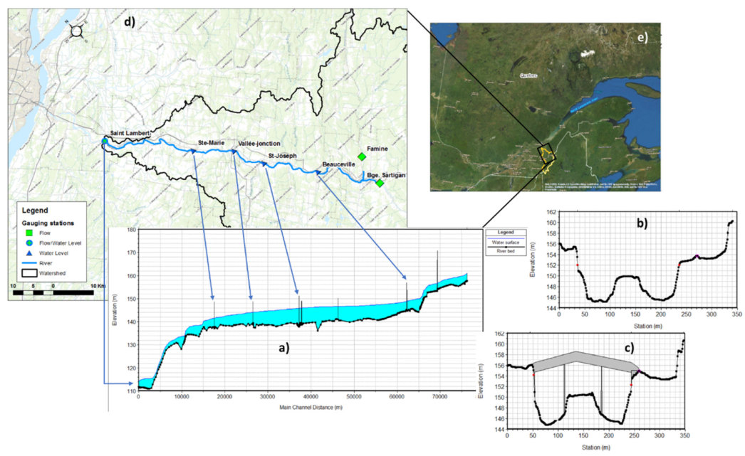
The Chaudière River takes its source in the Mégantic Lake located in southeastern Québec. It drains a watershed of 6694 km2 over a 200-km reach, before joining the St. Lawrence River near Quebec City. In its upstream part, the longitudinal profile of the river presents high to moderate slopes and intermittent rapids and cascades. In the downstream part, the stream network converges in the Beauce valley with slopes averaging only 0.05%, which lead to high flooding risk, particularly when it crosses the main urban developments (Figure 1).
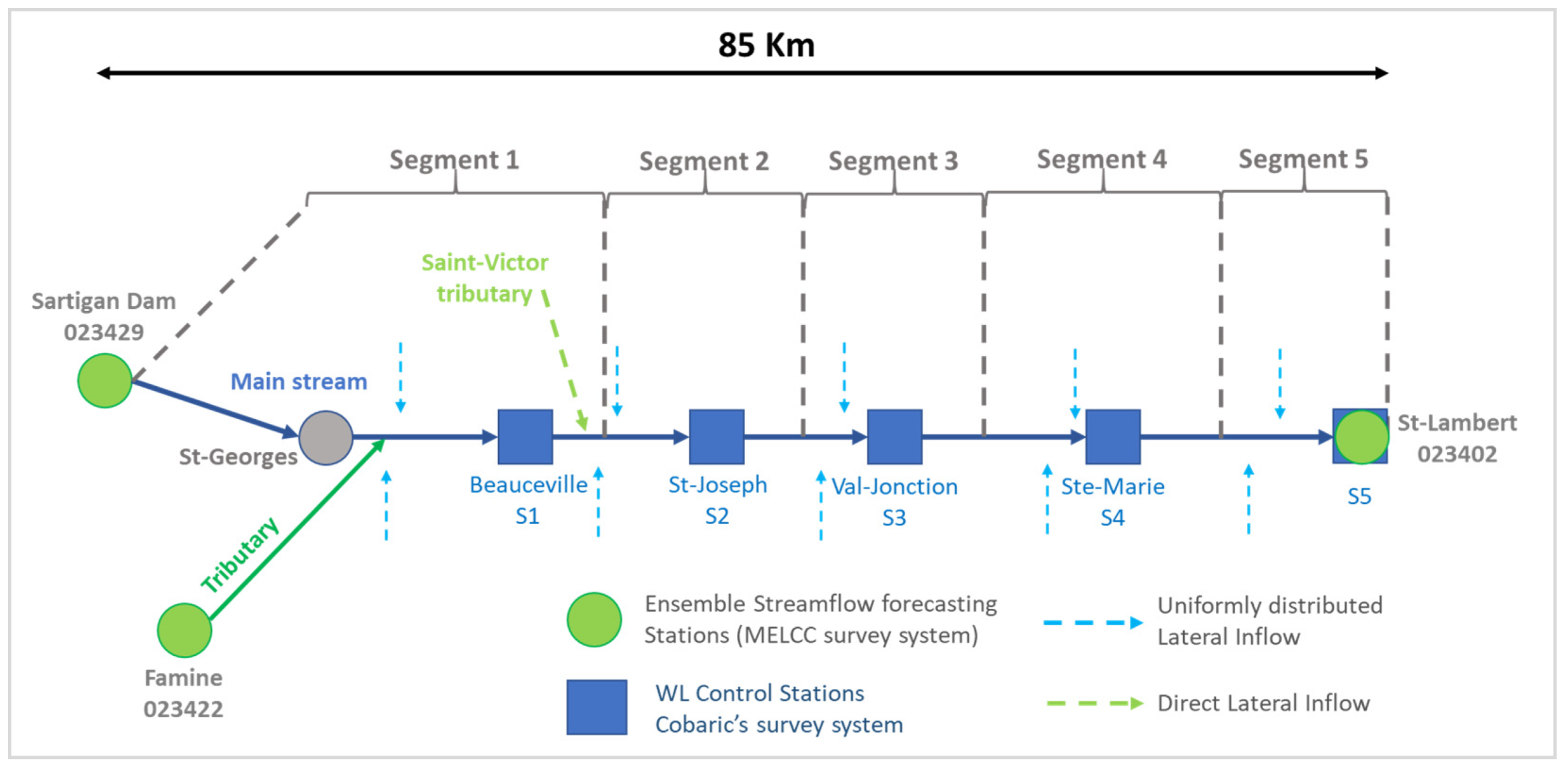
The hydraulic model focuses on the downstream part of the river (Figure 1). It extends over 85 km, from St-Georges to St-Lambert. The data necessary to build the model is provided by the MELCC (Ministère de l’Environnement et de la Lutte contre les Changements Climatiques). The geometry data were extracted from a digital elevation model (DEM) combining high-resolution (1 m × 1 m) Lidar and bathymetric data interpolated from several cross-section surveys distributed all along the river. Figure 2 summarizes the hydraulic model configuration and available data. The surveying network is composed of five water level (WL) stations (calibration points) controlled by the COBARIC (COmité de BAssin de la RIvière Chaudière) and distributed all along the reach and three gauging stations (WL/Q) controlled by the MELCC. Two of the gauging stations (Sartigan and Famine) are used directly as boundary conditions and the third one (St-Lambert) allows to estimate the lateral inflow from the intermediate basin.
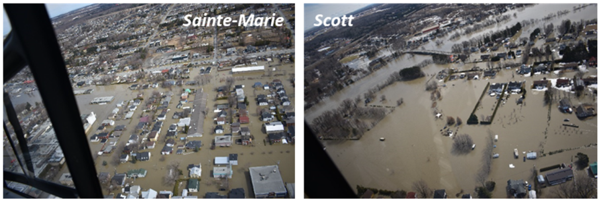
During spring 2019, the Chaudière River experienced historical flooding with an estimated flow (from a rating curve) at the St-Lambert station (the model outlet) of 2488 m3/s that exceeded the known 100-year return period (https://www.cehq.gouv.qc.ca/debits-crues/tableau-debits-crues.pdf). It is one of the largest free flow floods ever documented. Figure 3 illustrates the extent of the damage and flooding areas. The available data cover a wide range of flows that are very relevant to the present analysis, especially for its calibration process. Validation data focus on a 10-year return period event that occurred in spring 2018 with a peak flow at St-Lambert of 1908 m3/s. Other events are also considered in the calibration and validation processes with lower flow ranges and occurring during the summer and fall seasons; more details are given in the following paragraphs.
2.1.2. Hydraulic Model of the Chaudière River
HEC-RAS is a hydraulic modeling software widely used to address issues related to water level simulation and forecasting as well as floodplain delineation. The Chaudière River’s hydrodynamic model is built upon this tool to solve the 1D Saint-Venant equations. Even if it is not the prominent option for floodplain delineation, 1D modeling is very efficient in model implementation, computing time, and real-time operational forecasting [29]. HEC-RAS continuity (Equation (1)) and momentum (Equation (2)) equations are as follows [30]:
where Q is the flow (m3/s), AT is the total flow area (m2), ql is the lateral inflow per unit of length (m3/s/m), V is the velocity(m/s), A is the wetted area (m2), z/x is the water surface slope, Sf is the friction slope and g is the gravitational acceleration (m/s2).
The friction slope Sf (Equation (3)) [30] is the main term on which the model calibration is based by changing the Manning coefficient (n) value:
where Q is the flow(m3/s), R is the hydraulic radius (m), A is the wetted area (m2) and n is the Manning roughness coefficient (s/m1/3)
An implicit finite-difference scheme is used to calculate the water level, the flow, and velocities at every cross section [30]. In order to reproduce the geometry of the Chaudière River as accurately as possible, 295 cross-sections were extracted from the DEM with an average distance of 1 km and higher density around urban centers, hydraulic structures, and rapids. In addition, the 12 bridges present along the river were included in the river model, while respecting the dimensions of their various components (e.g., piers, deck, embankments); see Figure 1. To account for the 1D model limitations in dealing with flow storage in the floodplains and overflowing from the riverbed to flood prone areas, detailed levees and ineffective flow areas were defined for each cross section where applicable. Roughness coefficients, necessary to determine the friction term (Sf) of the momentum equation, were determined from available land use data; more details are given in the calibration section. Simulations for the calibration/validation process and the uncertainty analysis were performed in unsteady state to simulate water levels and flows all along the flood event, for every dataset. The dominant flow regime of the studied river stream is subcritical due to very mild slopes along the Beauce valley. A series of rapids are nonetheless present along the river causing local transitions to a critical flow regime. To deal with these transitions, simulations were run with a mixed flow regime option in order to stabilize the model through a local partial inertia (LPI) factor.
2.1.3. Calibration
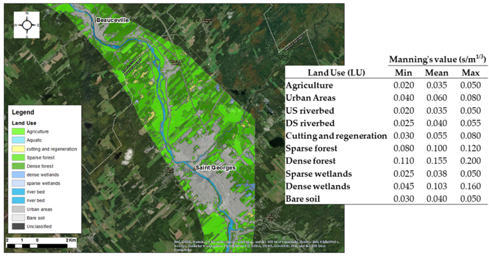
Roughness coefficient is important to hydraulic modeling, as it is one of the main tuning parameters used during the calibration process. Its determination depends on land use (LU) data. Reference values exist in the literature [31] so one can estimate ranges of roughness values according to the properties of the terrain.
Based on the available, detailed land use data, the study area was divided into several homogeneous roughness classes. They were next grouped into nine major categories as presented in Figure 4.
Xu et al. [15] considered the Manning roughness coefficient as an inherently time-varying model parameter that evolves over the course of a flood event and updated the calibrated values, according to pre-established linear relations, as a function of stage in real time. A similar approach is considered in this project to improve the precision of the hydraulic model for different events or flow regimes, e.g., when overflowing to the floodplains. To adapt this method to our hydraulic model (HEC-RAS) we adopted a calibration procedure using flow-varying adaptive roughness factors. These adjustment factors (nfac) are determined with HEC-RAS by automatic calibration for defined flow ranges (with a step of 100 or 200 m3/s) for each segment of the river where observed water level data are available; see Figure 2 for segments location. The mean absolute error (MAE) [32] is used as an optimization criterion (Equation (4)) in order to identify these adaptive roughness factors (nfac) by minimizing the following function to values ranging between 0.10 and 0.20 m.
where WLi sim is the simulated water level at time ti, WLi obs is the observed water level at the same time, and n is the total number of observations available for a given event and site. Since we have water level and flow measurements every 15 min, the deterministic performance metric (MAE) also informed us of the model’s ability to reproduce reality all along the flood event, including peak timing and flood routing errors.
In order to improve the efficiency of the approach, we applied the procedure to four flood events of various magnitudes (low, medium, and high) that occurred in spring, summer, and fall to account for flow regime and seasonal variability (Table 1). Figure 5 illustrates the hydrographs corresponding to the calibration and validation events, for the main control stations. Some hydrographs, mainly Sartigan Dam (red line) and the estimated lateral inflows (black line), show some abrupt variations due to regular controls on Sartigan Dam upstream that influence sharply the flow value. The impact on the model results are limited because the lateral inflow is distributed all along the river. The calibration is processed sequentially by segment from downstream to upstream assuming that the overall regime in the river is subcritical (very mild slope) and for each considered event, see Figure 6. The adaptive roughness factors relationships nfacij = f(Q) are thus established for every segment i and event j, depending on available observed WL data (automatic calibration). Each roughness category, as determined by land use classification, see Figure 4, participates in the roughness-flow relationships obtained and for each flow class considered. For example, if we take a typical section where the flow in the riverbed includes flow classes 0–1000 m3/s; the nfac adjustment factors obtained are related to the Manning of the riverbed. From a given threshold, e.g., Q > 1000 m3/s, flow will occur in the floodplains and a second, or third, roughness category will be included in the compilation of the friction term and thus the equivalent Manning of the section. Thus, the nfac adjustment factor for this flow class (e.g., 1000–2000 m3/s) will consider the new roughness category to contribute in the calibration process in conjunction with the Manning of the riverbed. The adopted relationships nfac = f(Q) for each segment are mainly derived from a weighting of the values obtained for each event and flow class. To ensure the consistency of the considered roughness factors, the calibration events are simulated using the resulting relationships in order to evaluate the overall performance of the model, and some minor adjustments can be made to improve the modeling results.
The river model accuracy is next assessed on common deterministic metrics: Mean Error or bias (ME) (Equation (5)), Mean Absolute Error (MAE) (Equation (4)), and Root Mean Square Error (RMSE) (Equation (6)) [32].
where Var is the variable of interest (WL or Q).
The adaptive, flow-based, roughness coefficients calibration can be considered as a sequential assimilation of the model parameters according to the observed or predicted inflow depending on the study objectives.
2.2. Uncertainty Analysis
Many sources of uncertainty affect the hydraulic modeling processes and several studies already addressed this issue [11,20,22,28,29]. In this project, we are focusing on the inputs of the model, namely the measured inflows and estimated lateral inflows, as well as the roughness coefficients.
2.2.1. Accounted Sources of Uncertainty
Observed and Measured Data Uncertainty
Most of the flow data series available and used as inputs in hydraulic or hydrological modeling are derived from rating curves. Flow hydrographs calculated by means of rating-curves are often used as uncertainty-free upstream boundary conditions [33]. The uncertainty in discharge measurement depends on multiple operational factors related, e.g., to the measurement methodology and instrumentation or the geometric properties of the control section or river, and may sometimes be as high as 20% of the observation [34]. The accuracy of the water level h(t) to flow Q(t) relationship that defines a rating curve also depends on the number of available field observations and the mathematical expression; as a result, interpolation and extrapolation errors are not negligible [33]. For example, average interpolation and extrapolation errors have been quantified, through steady state simulation, for the Po river as 1.7% and 13.8% of the flow Q(t), respectively [35].
It is therefore important to consider the inflow measurement error at the boundary conditions as one of the main sources of uncertainty. Since we are running the hydraulic model in unsteady state (with hysteresis effects) and due to the very mild slope (prone to backflow) of the Chaudière River, we considered an error of 10% on the inflow at the boundary conditions for the uncertainty analysis. The 10% error assumed is representative of the rating curve error, including associated water level measurements, flow measurements, and interpolation and extrapolation errors. The probabilistic scores presented in the Results section will confirm the adequacy of this estimation. On the other hand, the water level observations used for calibration are considered with a negligible error compared to model error.
Lateral Inflows
Lateral inflows are mostly ungauged and represent an important source of uncertainty in hydraulic modeling especially for large rivers with substantial lateral catchments. Lerat et al. [36] analyzed several assessments and application scenarios of lateral contributions using a linearized diffusive wave routing hydraulic model coupled to a hydrological model. The lateral contributions are estimated by modeling and applied either at the tributaries, uniformly distributed along the stream, or by combining the two options. The results showed that a uniform distribution of lateral flows led to performance values similar to those obtained with the maximum number of tributaries, with better stability in the calculations [36].
Due to the lack of lateral inflow measurements for the Chaudière River, it is important to evaluate the ungauged lateral inflows to the river and to check the routing performance at the model outlet. We developed a very simple and versatile approach to assess implicitly the intermediate volumes and to apply them uniformly or directly to the considered reach. The evaluation is based on the upstream and downstream-observed hydrographs and a prior evaluation of the routing performance values of the river for the accounted calibration events. The volume corresponding to the lateral inflows is derived by subtracting the routed upstream hydrographs from the observed one at the model outlet. Table 2 presents the area/weight distribution of each sub-basin of the Chaudière River. Note that the intermediate catchment represents more than one third of the total area.
The calculated hydrographs are then distributed into two lateral contributions. The first is uniformly distributed along the river, while the second is locally injected at the Saint-Victor tributary, with proportions of 60% and 40%, respectively (see Figure 2). To account for the uncertainty in the application of the lateral inflows, we considered several delays from 6 to 12 h in the uncertainty analysis. The lateral inflow uncertainty is also considered in addition to the proposed delays, accounting of the observation error associated to the Inflow, as described in paragraph Observed and Measured Data Uncertainty.
Roughness Parameters
The parameterization of the 1D river model is addressed through a land use (LU) based classification of the roughness coefficients for the riverbed and floodplains. In addition, five relationships were developed to adjust these coefficients according to the simulated flow for every river segment. Once the calibration of the hydrodynamic model is achieved through the adaptive roughness factors nfac, the proposed uncertainty associated to their determination should follow a Gaussian pdf with a mean value equal to calibrated nfac values and a standard deviation of 10% of the resulting values for each flow class and segment. The standard deviation considered is coherent with the values used by Xu et al. [15], around 8–11%.
2.2.2. Uncertainty Analysis Setup
To analyze the propagation of the uncertainty for the investigated sources, roughness coefficients, and inflows, we generated a set of parameters based on calibrated roughness factors relationships nfac = f(Q) and inflow observations, as well as on a prior quantification of their uncertainty. Knowing that random methods, such as Monte Carlo, are very demanding in terms of computation time. Considering the number of simulations required, we opted for a more controlled sampling approach. The uncertainty on the roughness factors and inflows is approached by the Latin Hypercube Sampling method (LHS) that generates random values with a better distribution in a defined uncertainty domain [19,26]. For the estimated lateral inflows application, considering the calibration/validation results of the hydrodynamic model, we explored 4 lag time values that are relevant to the model’s performance 6, 8, 10, and 12 h. With this set of parameters, a total of 10,000 combinations were produced and simulated to analyze the propagation of the uncertainty to the variables of interest. Figure 7 illustrates the proposed uncertainty framework and Table 3 summarizes the main characteristics of the considered sources of uncertainty.
2.2.3. Reliability Analysis
The reliability analysis of the uncertainty quantification is mandatory and relevant performance metrics are developed to assess it. In order to carry out this evaluation, we opt for the reliability diagram (Wilks, 2011) [24] and the Continuous Rank Probability Score (CRPS) [25] as probabilistic performance metrics. The CRPS (6) measures the difference between observations and predictions expressed as cumulative distributions functions [32]. For a given ith pair of observation-prediction ensemble, the CRPS is given by:
where F’i(x) is the predictive cumulative distribution function of the ith realization, x is the predicted variable, and H(x ≥ xi) is the Heaviside function where xi is the observed value. Since the CRPS is the probabilistic equivalent to the absolute error—the mathematical proof of this equivalence may be found in Baringhaus et al. and Székely et al. [37,38]—it has become a common procedure to compare the mean CRPS (MCRPS) and the MAE in order to assess the added value of a probabilistic (ensemble) approach over its deterministic counterpart [32].
A reliability diagram is constructed for each parameter (roughness, inflow) and their combination in order to assess their contribution to the uncertainty description. It provides a visual comparison of the observed and simulated probabilities for which the best performance is when the resulting line fits the reference (diagonal). In order to have a better interpretation of the reliability diagram, we are also interested in the ensemble spread (Equation (8)) of the resulting uncertainty analysis, as approximated by Fortin et al. [39], at the main control stations and how it compares to the model error, mainly the RMSE.
where si2 is the variance of the ith predictive distribution and si corresponds to its standard deviation.
3. Results
In this section, we present and discuss the outcomes of this study in two steps. First, the adaptive flow-based calibration and validation results are detailed highlighting the developed relationships. Performance is then assessed based on deterministic metrics, such as the mean error or bias (ME), the mean absolute error (MAE), and the root mean square error (RMSE). Second, the proposed uncertainty analysis targeting the propagation and quantification of the uncertainty and the resulting spread at the main control stations are analyzed. For simplification, we emphasize peak flow results and conclude with an analysis largely based on reliability diagrams.
3.1. Model Calibration and Validation
3.1.1. Adaptive Flow-Based Calibration Results
The adaptive flow-based calibration, performed over 4 events and applied to every river segment depending on data availability, allowed the development of five relationships nfac = f(Q) that express the adaptive roughness factor (nfac) as a function of the flow (Q) as illustrated in Figure 8. Final values by segment are established over a weighing based on calculated adaptive factors for each event and flow class. In some cases, weighing was not efficient, and we adopted some events roughness factors over others for better performance. The best illustration is for segment 5 (Saint-Lambert) where event 4 roughness factors were adopted over event 3 results (Figure 8). For other segments, similar adjustments were minor or absent, and all weighed values were considered. Relationships drawn in Figure 8 show that adaptive factors generally increase with flow. Such tendency is expected since higher flows result in higher water levels, increasing chances that parts of the flow take place through the denser vegetation of the floodplain. Resulting factors (nfac) are also highly sensitive to the segment flow (Q), with an average difference of 0.43 between minimum and maximum values. In addition, the resulting factors are typically smaller than one, except for segment 3, showing that reference values of the Manning coefficient are positively biased and do not match reality in this case. Calibrated values tend to vary between the minimum and average values proposed by Chow [31] (see Figure 4), according to the flow rate conveyed by each segment. Some exceptions are, however, noted for low flows (≤300 m3/s) in segment 1 (Beauceville) and 2 (St-Joseph) where the corresponding Manning coefficients are very low (0.011–0.012) and also for segment 3 (Vallée-Jonction) where the factors (nfac) are the highest. These exceptions show that the river model compensates for inconsistent bathymetric data and/or model structural errors through the Manning coefficients in order to reduce the overall model error, although with a risk of increasing model instability.
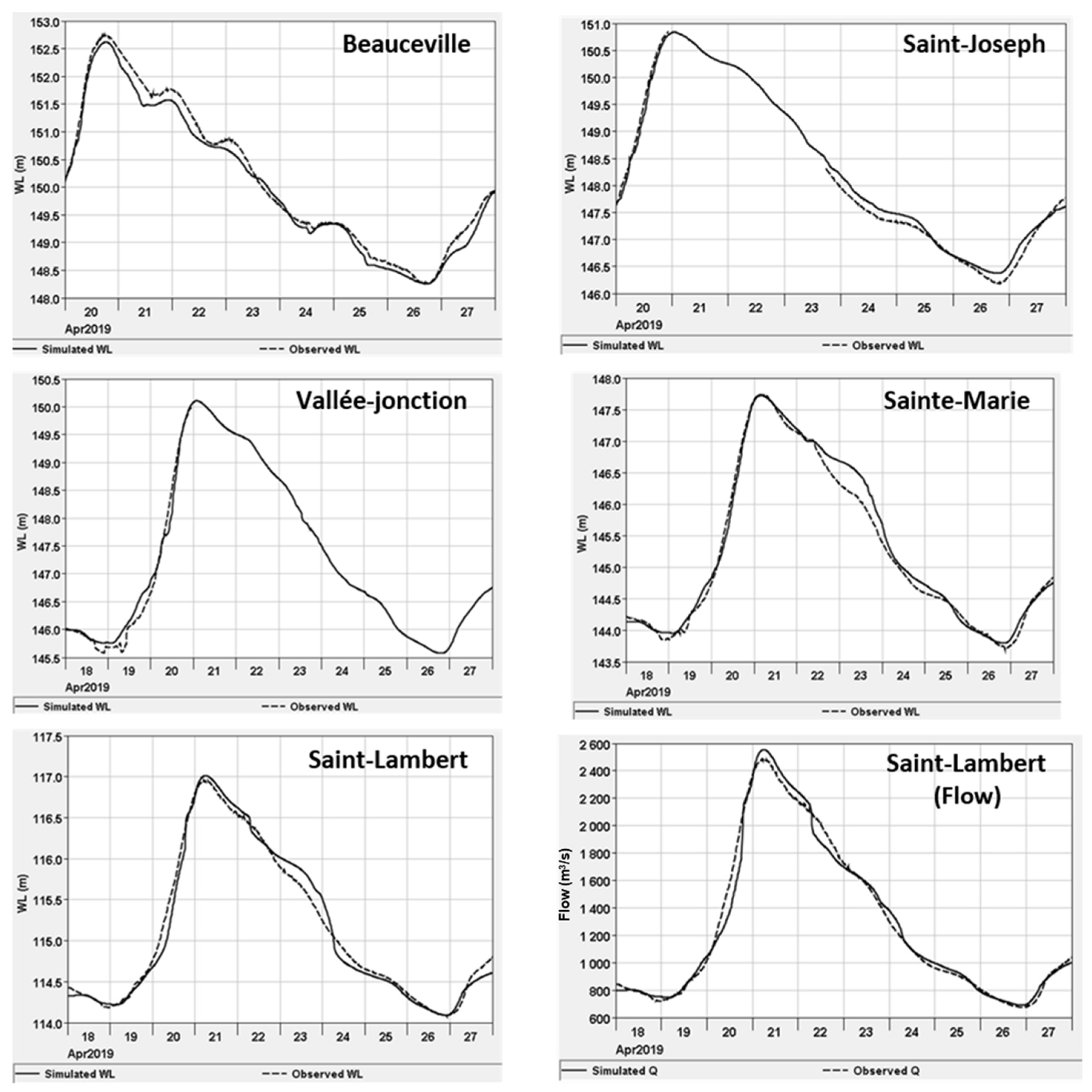
The river model calibration performance values are summarized in Table 4, using the final nfac = f(Q) relationships developed for each segment. Overall, results are quite good with limited ME or bias ranging between −0.12 and 0.07 m, except at Beauceville for event C1, where a positive bias of 0.18 cm is calculated. This systematic bias is due to the inability of the model to refine the calibration beyond the Manning values assumed for event C1, which is characterized by the lowest flow rates among the considered events. This confirms that for low flows, and for given segments, bathymetric data are not very accurate and calibrated coefficients cannot compensate for it at the expense of model instability. The MAE and RMSE are also quite satisfactory with respective values of 0.05 to 0.20 m and 0.07 to 0.22 m. The MAE and RMSE values for event C3 at segment 2 (St-Joseph) and 3 (Vallée-Jonction) are particularly high due to limited observed data available for calibration in comparison to event C4. As such, the weighted factors (nfac) impact heavily the results for event C3. In terms of flow, and regarding the outlet hydrograph (St-Lambert), the simulated flows present low bias and reasonable MAE (1.6–4.5%) and RMSE (2.5–7%) values, compared to peak flow values. To illustrate the main results, we present in Figure 9 the simulated and observed values for calibration event C4, which is the most important. Besides quantitative indicators of the river model performance, we can observe that the shape of the simulated and observed values are similar, with a good agreement on the peaks.
3.1.2. Validation Results
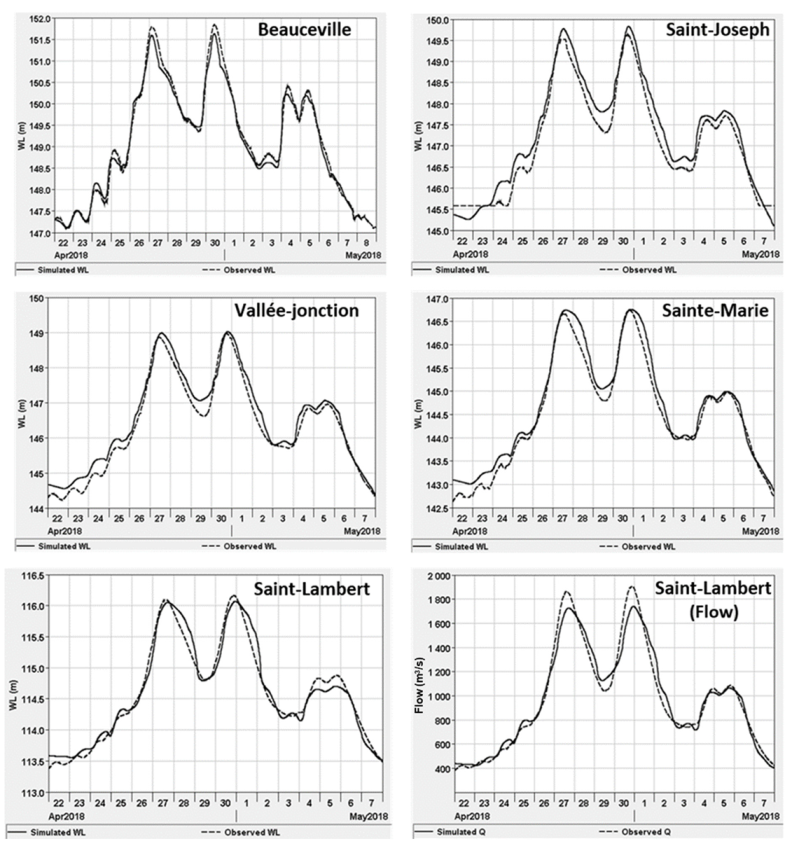
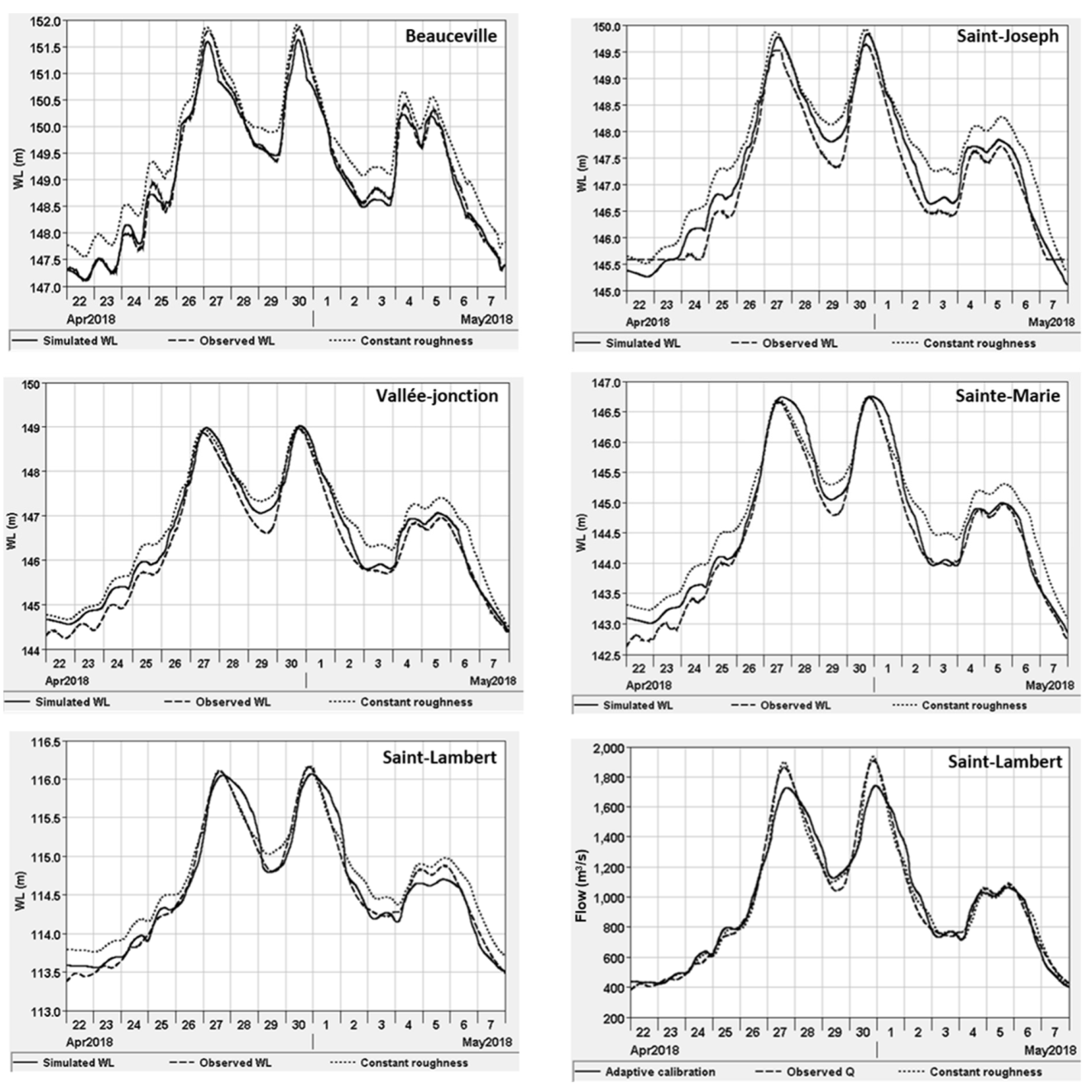
The adaptive flow-based relationships developed during the calibration process have been applied to two independent validation events of moderate and high importance. The Chaudière River model performs as well as during the calibration, except for station St-Joseph and Vallée-Jonction on event V2 where positive biases of 0.27 and 0.18 m occur, respectively. The systematic errors noted at those two stations can be attributed to a biased lateral inflow distribution for this event, since the tributary lateral inflow is applied at segment 2 upstream of the St-Joseph station. Indeed, an overestimation of the lateral inflow implies an inflated segment flow and subsequently biased water levels. It is also important to note here that the relationships developed for segments 2 and 3 are based on less events and the available data do not cover all the event duration. In addition, very low roughness factors for low flow classes are obtained, which is a sign, as discussed before, of poor bathymetry data. These errors can be improved by refining our calibration; however, it is interesting to see if our uncertainty analysis, afterward, would encompass this error. Table 4 summarizes the detailed performance values and Figure 10 illustrates simulated and observed WL and Q on the control sites and validation scenarios.
The adaptive flow-based calibration offers a built-in update to the model parameters (see Appendix A for comparison between constant and adaptive Manning calibration). The overall results reveal that the use of constant Manning coefficients will inevitably result in poorer results and larger water level error all along flood events, which is critical in a flooding context, even if the outflow hydrograph can be better reproduced with a constant Manning value, e.g., for event V2 (Figure A1, Appendix A). This indicates that the representation of the river geometry, and specifically the bathymetry, is not very accurate, and the proposed parameterization compensates for this error by optimizing the representation of water levels at the expense of a less accurate simulated outflow. Whether in calibration or validation, the performance of the model is variable in space and time, and the integration of the error, due to the identified sources of uncertainty, is necessary for a better understanding of model behavior. The following sections describe the key outcomes of the implemented uncertainty analysis and the propagation of the error through the variables of interest.
3.2. Uncertainty Analysis
In the following, we synthetize the main outcomes of the uncertainty quantification and evaluation. The analysis is applied to the validation’s main event V2 and the parametric error propagation to the variables of interest is assessed based on the identified sources of uncertainty. The selection of this event is driven by the covered flow range as well as modeling error that is higher than for event V1. The water level variable (WL) will be replaced by the water depth (D) in the analysis of uncertainty to make the related statistical moments—mainly the coefficient of variation (standard deviation/mean)—easier to interpret and comparable between control sections.
3.2.1. Quantification of the Uncertainty
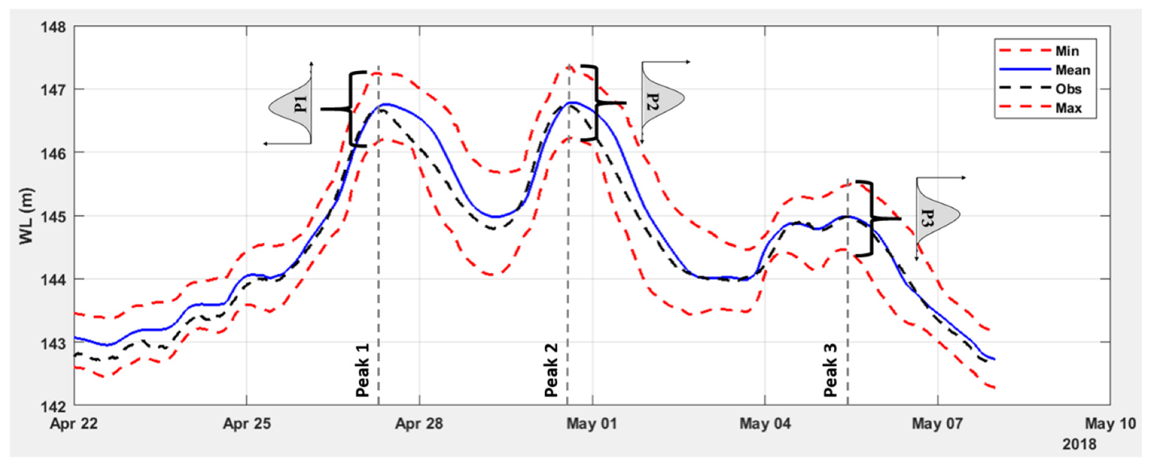
In order to simplify the analysis and presentation of the results, only three points, corresponding to the peak flows, will be considered below. The downside of this assumption is that the ensemble peaks do not occur at the same moment and we consider in the following that the impact on the dispersion is not significant. Figure 11 illustrates these points on a typical hydrograph for the analyzed event. For each of these peaks, we are interested in the resulting distributions (p1, p2, and p3) of the variables of interest through the assessment of characteristic properties, such as the mean μ, the standard deviation σ, and the coefficient of variation Cv (%) = σ/μ.
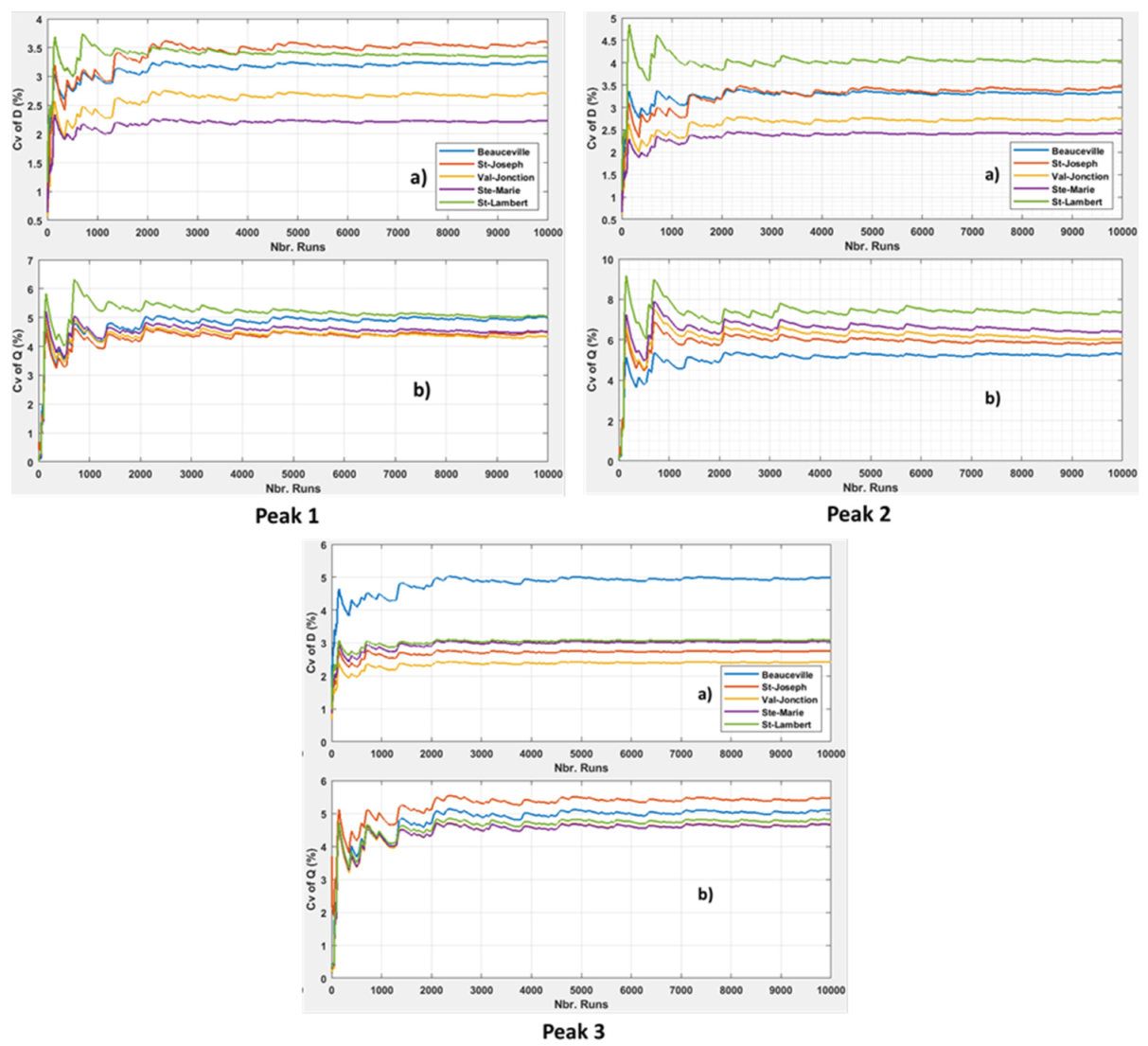
The proposed uncertainty framework, with its 10,000-parameter combinations, allows us to calculate moments for depth and flow on all the control stations. Figure 12 illustrates the moving average of the coefficient of variation CV (%) and Table 5 summarizes the resulting distribution characteristics on the three considered peak flows for water depth (D) and flow (Q). The water depth (D) is derived by subtracting the cross-section’s bottom level from the simulated water level (WL). On one hand, the first two moments (mean and standard deviation) of water depth are very close for peaks 1 and 2 for all stations, except for St-Lambert, where a higher variation is recorded for peak 2, with a standard deviation of 0.19 m compared to 0.15 m for peak 1 (see Table 5). This indicates that the description of uncertainty is stable over time under the same conditions (flows). The spatial variability is also very close with coefficients of variation that range from 2.2% to 5% for the considered peak flows and control stations. The resulting distributions are fairly symmetrical, with skewness values from −0.31 to 0.28 in most situations, except at St-Joseph (peak 1 and 2) and St-Lambert (peak 2), where the distributions are moderately skewed with values of −0.55 and 0.79. The kurtosis values given here are to compare the allure of our distributions to the normal one for which the kurtosis is equal to 3. Overall, the compiled kurtosis values are close to 3 and range from 2.66 to 3.16. The highest gap is recorded at St-Lambert for peak 2 with a value of 3.65, which is paired with a high positive skewness of 0.79, meaning a longer right tail for the distribution and a mean value lower than the mode. On the other hand, for the flow, the coefficients of variation are higher than for water depth and range from 4.3% to 7.3% with the highest values associated to peak 2. The spatial variability is also comparable between the considered stations as for water depth. Except for peak 3 at Beauceville, distributions on the remaining control points, especially for the higher flows (peak 2), are highly skewed with positive values that can reach up to 0.95 to 1.53, with an ascending gradient from upstream to downstream. These values are also correlated to high kurtosis values of 4.12 to 5.11, with larger right tails and peaked distributions.
Overall, we can assume that even with a Gaussian description of the error associated to the considered sources of uncertainty, the propagation of the error to variables of interest (WL and Q) does not necessarily result in a uniform distribution in all situations, and more pointy and asymmetric shapes are produced, depending essentially on the flow. It can also be noted that this trend applies more to the flow variable than to the water depth.
3.2.2. Reliability Analysis
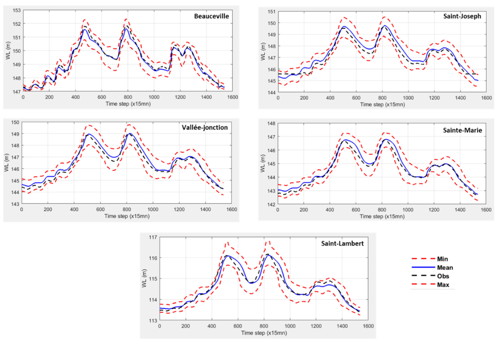
In the previous section, we evaluated the propagation of the uncertainty to the variables of interest (WL and Q) and, as illustrated in Appendix B, the set-up analysis with the accounted sources of uncertainty encompass very well the observed water level for most control stations. In the following, we focus on the accuracy and reliability of the uncertainty description using the mean continuous rank probability score (MCRPS) and reliability diagrams (RD). Results are also decomposed by parameter to determine the contribution of each in the dispersion produced.
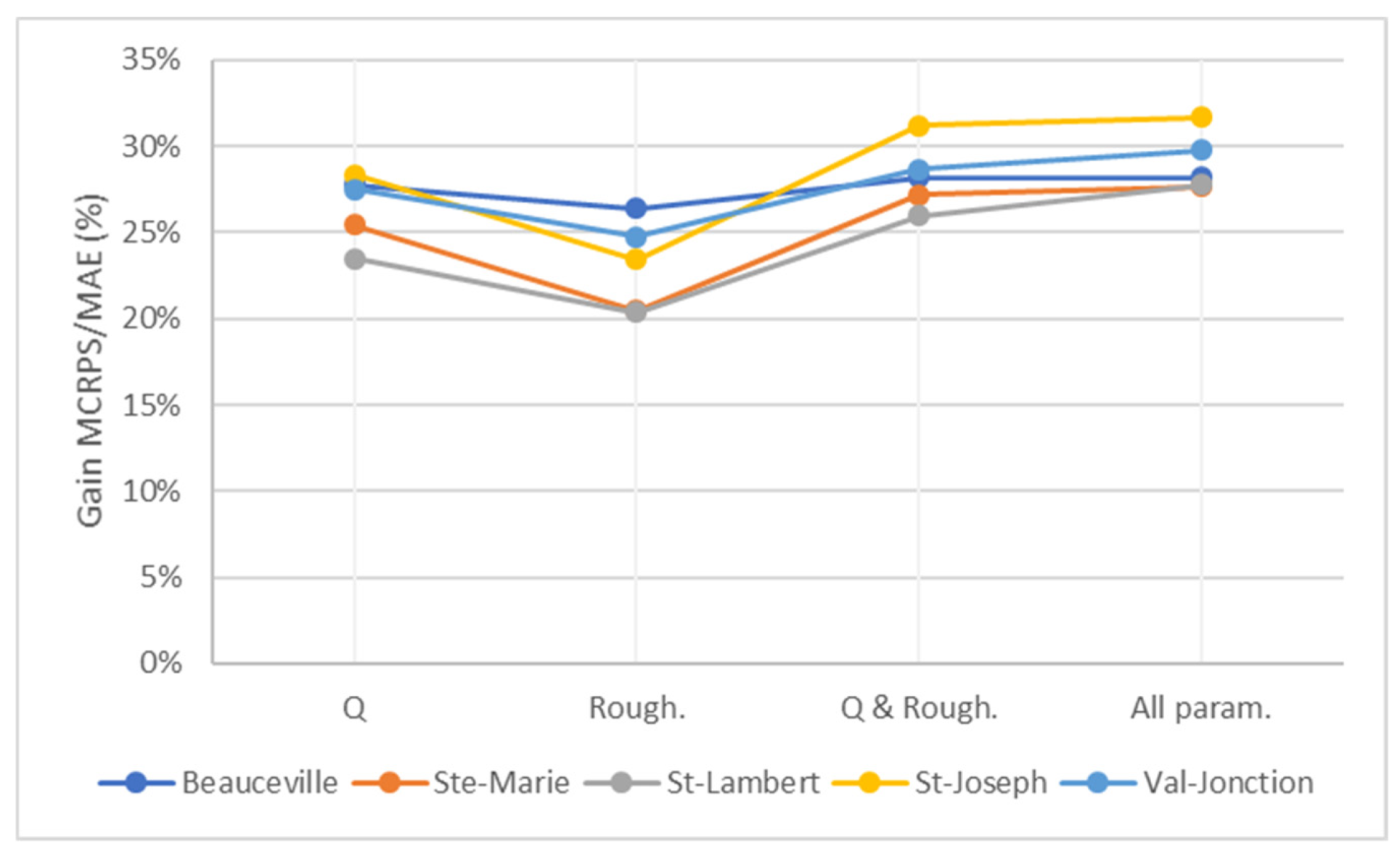
As already mentioned in Section 2.2.2, we compare the MCRPS and the MAE in order to assess the added value of the uncertainty analysis over its deterministic counterpart. Figure 13 illustrates the MCRPS gain (%) over the MAE for every parameter combination, and at each station involving as sources of uncertainty the flow Q, the calibrated roughness coefficients (Rough), a combination of both (Q & Rough) and all parameters including delays applied to the lateral inflows. The MAE here is calculated from the mean of each ensemble combination. We note that when considering parametric uncertainty, the resulting gains of accuracy range from 20% to 32% over a deterministic simulation. The values vary spatially and from one parameter to another. For example, the flow provides better gains (up to +5%) over roughness coefficients and is also very close to the combination of both parameters. The most significant gains from this uncertainty analysis are recorded at the stations where the deterministic model performs the least well, namely St-Joseph and Vallée-Jonction. We also note that the gain related to the application of a delay to the lateral inflow is quasi null except for station Vallée-Jonction and St-Joseph, which are located downstream of the direct lateral inflow at Saint-Victor tributary, and the outflow station St-Lambert.
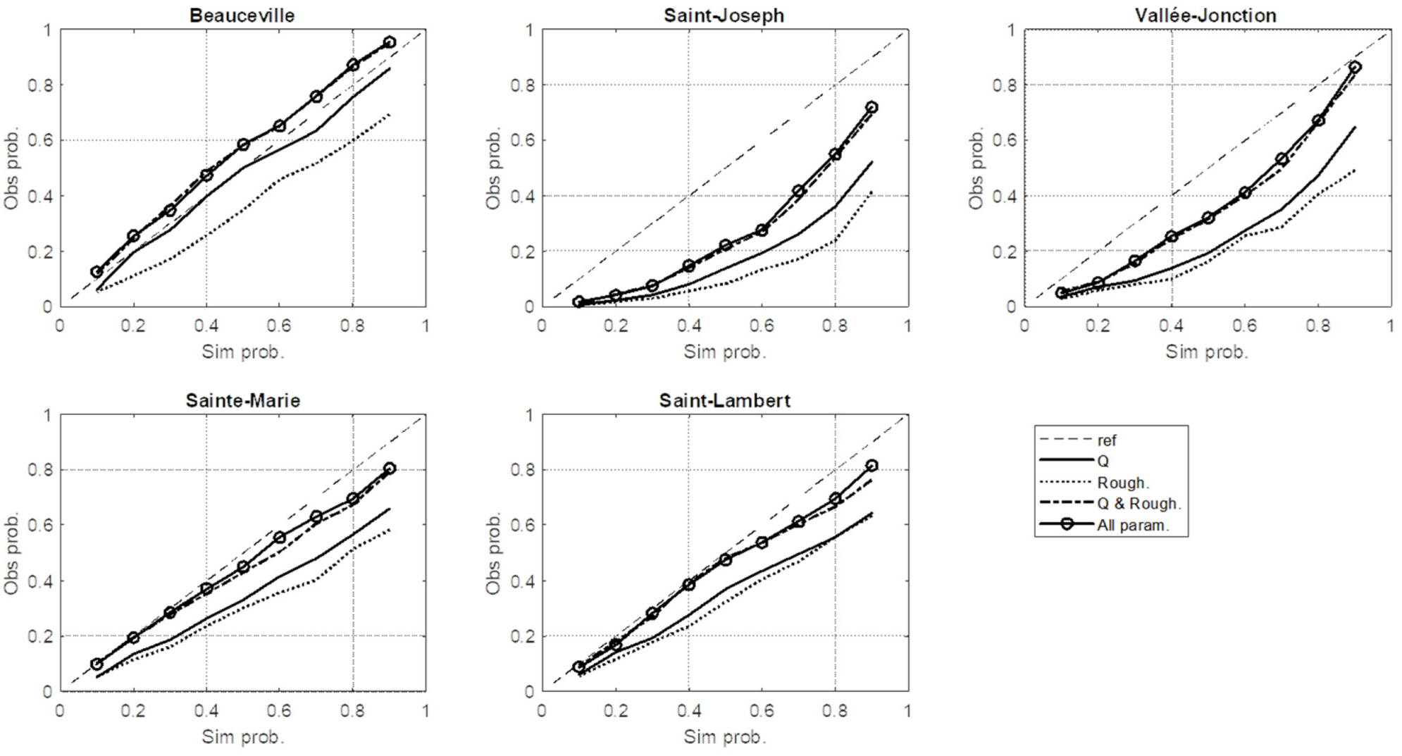
Reliability diagrams compiled at each station and accounted sources of uncertainty are illustrated in Figure 14. On one hand, results show that, at station Beauceville, Ste-Marie, and St-Lambert, the present uncertainty analysis, encompassing all parameters, is reliable: lines are very close to the reference. However, a light over-dispersion is noted at station Beauceville for which a better reliability is achieved when accounting only for flow uncertainty. At Ste-Marie and St-Lambert, a slight under-dispersion is noted at the extremes of the simulated distribution ending with simulated probabilities lower than the observed ones. On the other hand, the spread of the distributions generated at St-Joseph and Vallée-Jonction are clearly under-dispersed especially at St-Joseph. This outcome means that, despite the largest gain in MAE (Figure 13) obtained amongst all stations, our description of the uncertainty for these intermediate stations does not account for all local errors. By looking at the performances at these stations and compared to the resulting spreads through the uncertainty analysis (see Table 6), we can see that the spreads are lower than the RMSE of the river model, which confirms the interpretation of these reliability diagrams.
Overall, the flow parameter contributes more to the spread than the calibrated roughness coefficients, but their combined action leads to a better representation of the total model uncertainty; the influence of delays applied to the lateral inflows is very limited and localized in space. This is in accordance with the assumption that the 10% error associated with the determination of inflow is adapted to this type of analysis, especially when the performance of the calibrated model is close to the dispersion of the resulting ensemble. The reliability of the proposed uncertainty analysis varies also in space depending on the model performance at each segment and their sensitivity to the accounted sources. These findings show that in some sections of the model domain, additional sources of uncertainty, like lateral inflow distribution and the model structure, are to be considered to fully describe the uncertainty. For example, in this set-up we used a 1D hydraulic model that does not account explicitly for the floodplain dynamics (storage and side flows) as a 2D model would, and the methods used to represent them, such as ineffective flow areas and LPI factors, are not sufficient to fully address the structural uncertainty. These limitations of the hydraulic model are even more important for large flows with large floodplain overflows. The need for more detailed bathymetry data has also been noted during the calibration process for some segments where the resulting roughness coefficients were very low and outside of the reference domain. These limitations, due to the model structure and other potential parametric sources of uncertainty, might explain the observed discrepancies.
4. Conclusions
In this paper, we explored an adaptive flow-based calibration of a 1D hydraulic model of the Chaudière River, combined to an uncertainty analysis accounting for the errors associated to the calibrated roughness coefficients and the inflow. The resulting roughness/flow relationships allows updating Manning coefficients through adaptive roughness factors nfac as a function of flow, for every segment of the river, to minimize errors during a flood event. The model performance values over four calibration events were good, with RMSE and MAE below 20 cm for most of the control stations. Similar results were found for two validation events, except for event V2 where the considered lateral inflow distribution caused an overestimation of flow in segments 2 and 3, which resulted in larger RMSE values of 30 and 25 cm at station St-Joseph and Vallée-Jonction respectively. The developed roughness/flow relationships showed also some limitations of the model to compensate for poor bathymetry data in some segments where low values of Manning coefficients were obtained for the lowest flows. These relationships can be updated whenever additional data are available to improve their performance and have a better understanding of the associated error.
An uncertainty analysis was conducted based on validation event V2, for which the model was the least successful, accounting for the errors associated with inflow and adaptive roughness factors. The proposed framework, using controlled sampling, was successful in propagating the error to the variables of interest (water level and flow). The reliability analysis of the series showed that in terms of accuracy, a gain of 20% to 32% over a deterministic simulation was obtained. The flow error was the largest contributor to the spread, over roughness, for most control stations. The impact of the applied delays on the estimated lateral inflows was quite limited and localized. Reliability diagrams showed that for three of the control stations, the quantification of the uncertainty was reliable, with slightly over- or under-dispersed distributions. The uncertainty at the remaining stations, St-Joseph and Vallée-Jonction, affected by higher RMSE, revealed less reliable since the resulting spread did not fully catch up. Overall, the assumption of a 10% error in the flow determination was relevant in our analysis, especially when the model error and the dispersion of the ensemble are very close. These results highlight the fact that in some instances, an appropriate calibration combined to a good description of the parametric uncertainties may suffice to explain the variability in model outputs. However, in some cases, the model response and sensitivity to those parameters may vary both spatially and temporally, and additional (local or global) parametric or structural uncertainties might need to be included. For example, limitations of 1D hydraulic models in representing overbank flows may predominate over the considered parametric uncertainties in regions where floodplains occupy a significant proportion of the river section.
Depending on the purpose pursued throughout the development of a hydraulic model in a given area, the proposed framework can be adjusted to match the specific study objectives. Applications of such an approach could be found, for example, when developing ensemble flood warning and forecasting systems [40], which require fast and reliable responses and in which case a 1D hydraulic model can be efficiently applied with a controlled sampling strategy. The proposed nfac = f(Q) relationships are also a very good target for probabilistic data assimilation in the forecasting chain. In contrast, in the context of floodplain delineation, an adaptation of the uncertainty analysis approach for use with 2D hydraulic models should be foreseen. Other sampling methods can also be explored for computationally expensive applications (e.g., forecasting, 2D modelling), such as the point estimate method (PEM) and the perturbed moment method (PMM) [21].
Author Contributions
Conceptualization, M.A.B.; Methodology, M.A.B., P.M., and F.A.; Supervision, P.M. and F.A.; Validation, P.M. and F.A.; Writing—review & editing, M.A.B, P.M., and F.A.; Funding acquisition, F.A. All authors have read and agree to the published version of the manuscript.
Funding
This research was funded by FloodNet—an NSERC Canadian Strategic Network (Grant number: NETGP 451456) (http://www.nsercfloodnet.ca/).
Acknowledgments
Special thanks to the Ministère de l’Environnement et de la Lutte contre les changements climatiques (MELCC) of Québec for sharing the necessary data to build the river model and the Comité du bassin de la rivière Chaudière (COBARIC) for giving us access to the survey data over the river. We also thank Yves Secretan and two anonymous reviewers for reviewing the manuscript.
Conflicts of Interest
The authors declare no conflict of interest.
Appendix A. Water Level Series for Adaptive Flow-Based Calibration vs. Constant Manning Calibration vs. Observation—Validation Event V2
The figures below compare the different time series resulting from adaptive and constant Manning calibrations. The constant Manning calibration is optimized for peak flows and results are presented for validation event V2.
Figure A1.
Water level series for adaptive flow-based calibration (solid line) vs. constant Manning calibration (dotted line) vs. observation (dashed line).
Figure A1.
Water level series for adaptive flow-based calibration (solid line) vs. constant Manning calibration (dotted line) vs. observation (dashed line).

Appendix B. Simulated Water Level (WL) Ensembles vs. Observation at Each Station for Validation Event V2
Figure A2.
Water level ensembles vs. observations at each station—validation event V2.

References
- Neal, J.; Schumann, G.; Bates, P.; Buytaert, W.; Matgen, P.; Pappenberger, F. A data assimilation approach to discharge estimation from space. Hydrol. Process. 2009, 3649, 3641–3649. [Google Scholar] [CrossRef]
- Giustarini, L.; Matgen, P.; Hostache, R.; Montanari, M.; Plaza, D.; Pauwels, V.R.N.; De Lannoy, G.J.M.; De Keyser, R.; Pfister, L.; Hoffmann, L.; et al. Assimilating SAR-derived water level data into a hydraulic model: A case study. Hydrol. Earth Syst. Sci. 2011, 15, 2349–2365. [Google Scholar] [CrossRef] [Green Version]
- Giustarini, L.; Matgen, P.; Hostache, R.; Dostert, J. From SAR-derived flood mapping to water level data assimilation into hydraulic models. Remote Sens. Agric. Ecosyst. Hydrol. XIV 2012, 8531, 85310U. [Google Scholar]
- Andreadis, K.M.; Schumann, G.J.P. Estimating the impact of satellite observations on the predictability of large-scale hydraulic models. Adv. Water Resour. 2014, 73, 44–54. [Google Scholar] [CrossRef]
- Grimaldi, S.; Li, Y.; Pauwels, R.N.; Walker, J.P. Remote sensing-derived water extent and level to constrain hydraulic flood forecasting models: opportunities and challenges. Surv. Geophys. 2016, 37, 977–1034. [Google Scholar] [CrossRef]
- Matte, P.; Secretan, Y.; Morin, J. Hydrodynamic modeling of the St. Lawrence fluvial estuary I: model setup, calibration, and validation. J. Waterw. Port Coast. Ocean Eng. 2017, 143, 1–15. [Google Scholar] [CrossRef]
- Pappenberger, F.; Beven, K.; Horritt, M.; Blazkova, S. Uncertainty in the calibration of effective roughness parameters in HEC-RAS using inundation and downstream level observations. J. Hydrol. 2005, 302, 46–69. [Google Scholar] [CrossRef]
- Pappenberger, F.; Beven, K.; Frodsham, K.; Romanowicz, R.; Matgen, P. Grasping the unavoidable subjectivity in calibration of flood inundation models: A vulnerability weighted approach. J. Hydrol. 2007, 333, 275–287. [Google Scholar] [CrossRef]
- Di Baldassarre, G.; Schumann, G.; Bates, P.D.; Freer, J.E.; Beven, K.J. Flood-plain mapping: a critical discussion of deterministic and probabilistic approaches. Hydrol. Sci. J. 2010, 55, 364–376. [Google Scholar] [CrossRef]
- Barthélémy, S.; Ricci, S.; Rochoux, M.C.; Le Pape, E.; Thual, O. Ensemble-based data assimilation for operational flood forecasting—On the merits of state estimation for 1D hydrodynamic forecasting through the example of the “Adour Maritime” river. J. Hydrol. 2017, 552, 210–224. [Google Scholar] [CrossRef]
- Bates, P.D.; Pappenberger, F.; Romanowicz, R.J. Uncertainty in flood inundation modelling. In Applied Uncertainty Analysis for Flood Risk Management; World Scientific: Singapore, 2014; pp. 232–269. ISBN 9781848162716. [Google Scholar]
- Romanowicz, R.; Beven, K. Estimation of flood inundation probabilities as conditioned on event inundation maps. Water Resour. Res. 2003, 39. [Google Scholar] [CrossRef]
- Troy, T.J.; Wood, E.F.; Sheffield, J. An efficient calibration method for continental-scale land surface modeling. Water Resour. Res. 2008, 44, 1–13. [Google Scholar] [CrossRef]
- Acuña, G.J.; Ávila, H.; Canales, F.A. River Model Calibration Based on Design of Experiments Theory. A Case Study: Meta River, Colombia. Water 2019, 11, 382. [Google Scholar] [CrossRef] [Green Version]
- Xu, X.; Zhang, X.; Fang, H.; Lai, R.; Zhang, Y.; Huang, L.; Liu, X. A real-time probabilistic channel flood-forecasting model based on the Bayesian particle filter approach. Environ. Model. Softw. 2017, 88, 151–167. [Google Scholar] [CrossRef] [Green Version]
- Tung, Y. Uncertainty and Reliability Analysis in Water Resources Engineering. J. Contemp. Water Res. Educ. 2011, 103, 4. [Google Scholar]
- Kalyanapu, A.J.; Judi, D.R.; McPherson, T.N.; Burian, S.J. Monte Carlo-based flood modelling framework for estimating probability weighted flood risk. J. Flood Risk Manag. 2012, 5, 37–48. [Google Scholar] [CrossRef]
- Huang, Y.; Qin, X. Uncertainty analysis for flood inundation modelling with a random floodplain roughness. Environ. Syst. Res. 2014, 3, 9. [Google Scholar] [CrossRef] [Green Version]
- Goeury, C.; David, T.; Ata, R.; Boyaval, S.; Audouin, Y.; Goutal, N.; Popelin, A.-L.; Couplet, M.; Baudin, M.; Barate, R. Uncertainty quantification on a real case with TELEMAC-2D. In Proceedings of the XXII TELEMAC-MASCARET Technical User Conference, Warrington, UK, 15–16 October 2015; pp. 44–51. [Google Scholar]
- Altarejos-Garcia, L.; Martinez-Chenoll, M.L.; Escuder-Bueno, I.; Serrano-Lombillo, A. Assessing the impact of uncertainty on flood risk estimates with reliability analysis using 1-D and 2-D hydraulic models. Hydrol. Earth Syst. Sci. 2012, 16, 1895–1914. [Google Scholar] [CrossRef] [Green Version]
- Franceschini, S.; Marani, M.; Tsai, C.; Zambon, F. A perturbance moment point estimate method for uncertainty analysis of the hydrologic response. Adv. Water Resour. 2012, 40, 46–53. [Google Scholar] [CrossRef]
- Jung, Y.; Merwade, V.; Asce, M. Uncertainty quantification in flood inundation mapping using generalized likelihood uncertainty estimate and sensitivity analysis. J. Hydrol. Eng. 2012, 17, 507–520. [Google Scholar] [CrossRef]
- Beven, K.; Binley, A. The future of distributed models: Model calibration and uncertainty prediction. Hydrol. Process. 1992, 6, 279–298. [Google Scholar] [CrossRef]
- Wilks, D.S. Statistical Methods in the Atmospheric Sciences (International Geophysics); Academic Press: Cambridge, MA, USA, 2011; ISBN 978-0123850225. [Google Scholar]
- Gneiting, T.; Raftery, A.E. Strictly proper scoring rules, prediction, and estimation. J. Am. Stat. Assoc. 2007, 102, 359–378. [Google Scholar] [CrossRef]
- Lemieux, C. Monte Carlo and Quasi-Monte Carlo Sampling; Springer: New York, NY, USA, 2009; ISBN 9780387781648. [Google Scholar]
- Cea, L.; French, J.R. Bathymetric error estimation for the calibration and validation of estuarine hydrodynamic models. Estuar. Coast. Shelf Sci. 2012, 100, 124–132. [Google Scholar] [CrossRef]
- Hunter, N.M.; Bates, P.D.; Neelz, S.; Pender, G. Benchmarking 2D hydraulic models for urban flooding. Proc. Inst. Civ. Eng. Water Manag. 2008, 161, 13–30. [Google Scholar] [CrossRef] [Green Version]
- Costabile, P.; Macchione, F. Enhancing river model set-up for 2-D dynamic flood modelling. Environ. Model. Softw. 2015, 67, 89–107. [Google Scholar] [CrossRef]
- Brunner, G. HEC-RAS River Analysis System, Hydraulic Reference Manual, Version 5.0; US Army Corps of Engineers, Hydrologic Engineer Center (HEC): Davis, CA, USA, 2016. [Google Scholar]
- Chow, V.T. Open Channel Hydraulics; McGraw-Hill: New York, NY, USA, 1959. [Google Scholar]
- Anctil, F.; Ramos, M.-H. Verification Metrics for Hydrological Ensemble Forecasts. In Handbook of Hydrometeorological Ensemble Forecasting; Springer: Berlin/Heidelberg, Germany, 2018; pp. 1–30. ISBN 9783642404573. [Google Scholar]
- Domeneghetti, A.; Castellarin, A.; Brath, A. Assessing rating-curve uncertainty and its effects on hydraulic model calibration. Hydrol. Earth Syst. Sci. 2012, 16, 1191–1202. [Google Scholar] [CrossRef] [Green Version]
- Pelletier, M. Uncertainties in the single determination of river discharge: A literature review. Can. J. Civ. Eng. 1988, 15, 834–850. [Google Scholar] [CrossRef]
- Di Baldassarre, G.; Montanari, A. Uncertainty in river discharge observations: A quantitative analysis. Hydrol. Earth Syst. Sci. 2009, 13, 913–921. [Google Scholar] [CrossRef] [Green Version]
- Lerat, J.; Perrin, C.; Andréassian, V.; Loumagne, C.; Ribstein, P. Towards robust methods to couple lumped rainfall-runoff models and hydraulic models: A sensitivity analysis on the Illinois River. J. Hydrol. 2012, 418–419, 123–135. [Google Scholar] [CrossRef] [Green Version]
- Baringhaus, L.; Franz, C. On a new multivariate two-sample test. J. Multivar. Anal. 2004, 88, 190–206. [Google Scholar] [CrossRef]
- Székely, G.J.; Rizzo, M.L. A new test for multivariate normality. J. Multivar. Anal. 2005, 93, 58–80. [Google Scholar] [CrossRef] [Green Version]
- Fortin, V.; Abaza, M.; Anctil, F.; Turcotte, R. Why should ensemble spread match the RMSE of the ensemble mean? J. Hydrometeorol. 2014, 15, 1708–1713. [Google Scholar] [CrossRef]
- Thiboult, A.; Anctil, F.; Boucher, M.A. Accounting for three sources of uncertainty in ensemble hydrological forecasting. Hydrol. Earth Syst. Sci. 2016, 20, 1809–1825. [Google Scholar] [CrossRef] [Green Version]
Figure 1.
Location and geometry of the Chaudière River: (a) longitudinal profile of the river, (b) sample cross section of the 1D river model, (c) sample of the hydraulic structures included in the river model, (d) World Topographic Map—Sources: Esri, HERE, Garmin, Intermap, increment P Corp., GEBCO, USGS, FAO, NPS, NRCAN, GeoBase, IGN, Kadaster NL, Ordnance Survey, Esri Japan, METI, Esri China (Hong Kong), (c) OpenStreetMap contributors, and the GIS User Community, and (e) World Boundaries and Places–Esri, HERE, Garmin, (c) OpenStreetMap contributors, and the GIS user community. World Imagery–Source: Esri, DigitalGlobe, GeoEye, Earthstar Geographics, CNES/Airbus DS, USDA, USGS, AeroGRID, IGN, and the GIS User Community.

Figure 2.
Simplified configuration of the Chaudière River model.

Figure 3.
Extent of flooded areas: 21 April 2019.

Figure 4.
Roughness coefficients mapping according to land use (LU) classification for the Chaudière River.
Figure 4.
Roughness coefficients mapping according to land use (LU) classification for the Chaudière River.

Figure 5.
Calibration and validation hydrographs. Locations are schematically drawn in Figure 2.
Figure 5.
Calibration and validation hydrographs. Locations are schematically drawn in Figure 2.

Figure 6.
Adaptive calibration of the river model for each segment and event.

Figure 7.
Uncertainty analysis framework.

Figure 8.
Adaptive flow-based calibration relationships nfac = f(Q) developed for the model segments.
Figure 8.
Adaptive flow-based calibration relationships nfac = f(Q) developed for the model segments.

Figure 9.
Simulated and observed values for calibration event C4.

Figure 10.
Simulated vs. observed values for validation event V2.

Figure 11.
Location of the peak flow analysis on a typical generated hydrograph for the considered event V2.
Figure 11.
Location of the peak flow analysis on a typical generated hydrograph for the considered event V2.

Figure 12.
Moving average of the coefficient variation (CV) in % for depth (D) and flow (Q) at control stations (colored lines) for peak 1, 2, and 3: (a) Depth, (b) Flow.
Figure 12.
Moving average of the coefficient variation (CV) in % for depth (D) and flow (Q) at control stations (colored lines) for peak 1, 2, and 3: (a) Depth, (b) Flow.

Figure 13.
Mean continuous rank probability score (MCRPS) gain in % over the mean absolute error (MAE) for various locations and ensemble subsets.
Figure 13.
Mean continuous rank probability score (MCRPS) gain in % over the mean absolute error (MAE) for various locations and ensemble subsets.

Figure 14.
Reliability diagrams of simulation vs. observation probabilities at each control station for the considered parameters flow (Q), roughness coefficients (Rough), a combination of both, and all parameters combined.
Figure 14.
Reliability diagrams of simulation vs. observation probabilities at each control station for the considered parameters flow (Q), roughness coefficients (Rough), a combination of both, and all parameters combined.


Table 1.
Events considered in the calibration and validation processes.
| Process | Event | Start Date | End Date | Outflow | |
|---|---|---|---|---|---|
| Min (m3/s) | Max (m3/s) | ||||
| Calibration | Event C1 | 14 May 2016 | 22 May 2016 | 50 | 270 |
| Event C2 | 14 August 2016 | 16 August 2016 | 20 | 616 | |
| Event C3 | 17 August 2016 | 21 August 2016 | 75 | 950 | |
| Event C4 | 19 April 2019 | 27 April 2019 | 675 | 2488 | |
| Validation | Event V1 | 21 October 2016 | 26 October 2016 | 40 | 1085 |
| Event V2 | 22 April 2018 | 7 May 2018 | 400 | 1910 | |
Table 2.
Boundary conditions and ratio to the total catchment area.
| Station (Boundary Condition, BC) | Area (km2/(% Total Area)) |
|---|---|
| Sartigan Dam (upstream BC) | 3074 (52.8%) |
| Famine (tributary BC) | 696 (12%) |
| Intermediate catchments (lateral inflows) | 2050 (35.2%) |
| St-Lambert (downstream BC) | 5820 (100%) |
Table 3.
Characterization of the accounted sources of uncertainty.
| Source of Uncertainty | Mean | Standard Deviation | Method | Members |
|---|---|---|---|---|
| Inflow | Observation | +/−10% Mean | Latin Hypercube Sampling following a Gaussian pdf | 50 |
| Roughness | Calibrated nfac = f(Q) | 50 | ||
| Lateral Inflows (LI) | Estimated LI from Outflow minus Inflow | 4 delays proposed to catch the hydrograph allure and peak at the outlet. The same uncertainty as Inflow is applied with +/−10% of estimated LI. | 4 | |
| Parameters set | 10,000 | |||
Table 4.
Calibration and validation performance values per event and control site (Mean Error (ME), Mean Absolute Error (MAE), and Root Mean Square Error (RMSE)).
Table 4.
Calibration and validation performance values per event and control site (Mean Error (ME), Mean Absolute Error (MAE), and Root Mean Square Error (RMSE)).
| Stations | Performance | Calibration | Validation | ||||
|---|---|---|---|---|---|---|---|
| Event C1 | Event C2 | Event C3 | Event C4 | Event V1 | Event V2 | ||
| Beauceville | ME (m) | 0.18 | −0.01 | −0.02 | −0.12 | −0.06 | −0.05 |
| MAE (m) | 0.18 | 0.17 | 0.17 | 0.14 | 0.16 | 0.12 | |
| RMSE (m) | 0.20 | 0.19 | 0.22 | 0.16 | 0.20 | 0.15 | |
| St-Joseph | ME (m) | - | - | −0.12 | 0.07 | 0.08 | 0.27 |
| MAE (m) | - | - | 0.22 | 0.12 | 0.13 | 0.27 | |
| RMSE (m) | - | - | 0.25 | 0.14 | 0.18 | 0.30 | |
| Vallée-jonction | ME (m) | - | 0.03 | −0.10 | 0.06 | 0.05 | 0.18 |
| MAE (m) | - | 0.11 | 0.20 | 0.13 | 0.15 | 0.21 | |
| RMSE (m) | - | 0.12 | 0.27 | 0.18 | 0.20 | 0.25 | |
| Sainte-Marie | ME (m) | −0.02 | 0.01 | −0.02 | 0.07 | 0.04 | 0.13 |
| MAE (m) | 0.05 | 0.15 | 0.11 | 0.11 | 0.11 | 0.15 | |
| RMSE (m) | 0.07 | 0.18 | 0.18 | 0.15 | 0.15 | 0.21 | |
| Saint-Lambert (WL) | ME (m) | - | - | 0.04 | −0.01 | 0.03 | 0.00 |
| MAE (m) | - | - | 0.15 | 0.08 | 0.15 | 0.11 | |
| RMSE (m) | - | - | 0.17 | 0.11 | 0.16 | 0.15 | |
| Saint-Lambert (Q) | ME (m3/s) | - | - | 3.0 | −0.3 | 2.7 | −0.8 |
| MAE (m3/s) | - | - | 43.3 | 41.4 | 34.1 | 65.5 | |
| RMSE (m3/s) | - | - | 66.3 | 63.3 | 41.6 | 86.2 | |
Table 5.
Summary of uncertain water level and flow moments: mean (µ), standard deviation (σ), coefficient of variation (Cv), skewness (Sk), and kurtosis (Ku) for the considered peak flows and control stations.
Table 5.
Summary of uncertain water level and flow moments: mean (µ), standard deviation (σ), coefficient of variation (Cv), skewness (Sk), and kurtosis (Ku) for the considered peak flows and control stations.
| Stations | Checkpoint | Depth | Flow | ||||||||
|---|---|---|---|---|---|---|---|---|---|---|---|
| µ (m) | σ (m) | Cv (%) | Sk | Ku | µ (m3/s) | σ (m3/s) | Cv (%) | Sk | Ku | ||
| Beauceville | Peak 1 | 5.74 | 0.19 | 3.25 | −0.27 | 2.77 | 1090.0 | 54.6 | 5.01 | 0.03 | 2.87 |
| Peak 2 | 5.82 | 0.19 | 3.34 | −0.07 | 3.03 | 1128.0 | 59.9 | 5.31 | 0.30 | 3.18 | |
| Peak 3 | 4.72 | 0.24 | 4.99 | −0.31 | 2.78 | 734.3 | 37.4 | 5.09 | −0.29 | 2.59 | |
| St-Joseph | Peak 1 | 8.94 | 0.32 | 3.60 | −0.50 | 2.66 | 1466.7 | 65.9 | 4.49 | 0.20 | 3.76 |
| Peak 2 | 9.07 | 0.31 | 3.46 | −0.55 | 2.87 | 1535.4 | 89.7 | 5.84 | 0.95 | 4.12 | |
| Peak 3 | 7.11 | 0.20 | 2.76 | 0.23 | 3.08 | 913.2 | 49.9 | 5.46 | −0.11 | 2.34 | |
| Vallée-jonction | Peak 1 | 10.57 | 0.29 | 2.70 | −0.27 | 2.88 | 1577.6 | 68.4 | 4.34 | 0.57 | 3.23 |
| Peak 2 | 10.67 | 0.29 | 2.75 | −0.21 | 2.72 | 1622.3 | 97.7 | 6.02 | 1.16 | 4.43 | |
| Peak 3 | 8.66 | 0.21 | 2.42 | 0.05 | 2.99 | 976.8 | 45.7 | 4.67 | 0.15 | 2.88 | |
| Sainte-Marie | Peak 1 | 7.32 | 0.16 | 2.23 | 0.00 | 3.16 | 1639.4 | 73.9 | 4.51 | 0.60 | 2.97 |
| Peak 2 | 7.34 | 0.18 | 2.43 | 0.08 | 2.89 | 1676.2 | 107.1 | 6.39 | 1.24 | 4.72 | |
| Peak 3 | 5.54 | 0.17 | 3.05 | 0.01 | 2.86 | 1007.5 | 47.0 | 4.66 | 0.23 | 2.78 | |
| Saint-Lambert | Peak 1 | 4.60 | 0.15 | 3.36 | 0.28 | 2.96 | 1754.8 | 88.5 | 5.05 | 0.73 | 3.36 |
| Peak 2 | 4.61 | 0.19 | 4.04 | 0.79 | 3.65 | 1762.7 | 129.3 | 7.33 | 1.53 | 5.11 | |
| Peak 3 | 3.22 | 0.10 | 3.10 | 0.11 | 2.67 | 1063.8 | 51.3 | 4.82 | 0.11 | 2.57 | |
Table 6.
Spread and RMSE at each site.
| Station | Spread (m) | RMSE (m) | % RMSE |
|---|---|---|---|
| Beauceville | 0.17 | 0.14 | 123% |
| St-Joseph | 0.22 | 0.29 | 76% |
| Vallé-Jonction | 0.23 | 0.27 | 83% |
| Ste-Marie | 0.19 | 0.20 | 91% |
| St-Lambert | 0.13 | 0.15 | 87% |
© 2020 by the authors. Licensee MDPI, Basel, Switzerland. This article is an open access article distributed under the terms and conditions of the Creative Commons Attribution (CC BY) license (http://creativecommons.org/licenses/by/4.0/).
Share and Cite
MDPI and ACS Style
Bessar, M.A.; Matte, P.; Anctil, F. Uncertainty Analysis of a 1D River Hydraulic Model with Adaptive Calibration. Water 2020, 12, 561. https://doi.org/10.3390/w12020561
AMA Style
Bessar MA, Matte P, Anctil F. Uncertainty Analysis of a 1D River Hydraulic Model with Adaptive Calibration. Water. 2020; 12(2):561. https://doi.org/10.3390/w12020561
Chicago/Turabian StyleBessar, Mohammed Amine, Pascal Matte, and François Anctil. 2020. "Uncertainty Analysis of a 1D River Hydraulic Model with Adaptive Calibration" Water 12, no. 2: 561. https://doi.org/10.3390/w12020561
Note that from the first issue of 2016, this journal uses article numbers instead of page numbers. See further details here.