Article

Hydrological Foundation as a Basis for a Holistic Environmental Flow Assessment of Tropical Highland Rivers in Ethiopia

1
Amhara Design and Supervision Works Enterprise, Bahir Dar, P.O. Box 1921, Ethiopia
2
Faculty of Civil and Water Resources Engineering, Bahir Dar Institute of Technology, Bahir Dar University, Bahir Dar, P.O. Box 26, Ethiopia
3
School of Fisheries and Wildlife, Department of Aquatic and Wetland Management, Bahir Dar University, Bahir Dar, P.O. Box 26, Ethiopia
4
Basin Information System Directorate, Abbay River Basin Authority, Bahir Dar, P.O. Box 1376, Ethiopia
5
Department of Biological and Environmental Engineering, Cornell University, Ithaca, NY 14850, USA
6
Laboratory for Applied Geology and Hydrogeology, Ghent University, Pietersnieuwstraat 33, 9000 Gent, Belgium
7
Department of Water Resources and Ecosystems, IHE Delft Institute for Water Education, Westvest 7, 2611 AX Delft, Países Baixos, The Netherlands
8
Faculty of Civil Engineering and Geosciences, Delft University of Technology, Mekelweg 5, 2628 CD Delft, Países Baixos, The Netherlands
*
Author to whom correspondence should be addressed.
Water 2020, 12(2), 547; https://doi.org/10.3390/w12020547
Submission received: 16 December 2019 / Revised: 11 February 2020 / Accepted: 13 February 2020 / Published: 15 February 2020
(This article belongs to the Special Issue A Systems Approach for River and River Basin Restoration)

Abstract

:
The sustainable development of water resources includes retaining some amount of the natural flow regime in water bodies to protect and maintain aquatic ecosystem health and the human livelihoods and wellbeing dependent upon them. Although assessment of environmental flows is now occurring globally, limited studies have been carried out in the Ethiopian highlands, especially studies to understand flow-ecological response relationships. This paper establishes a hydrological foundation of Gumara River from an ecological perspective. The data analysis followed three steps: first, determination of the current flow regime—flow indices and ecologically relevant flow regime; second, naturalization of the current flow regime—looking at how flow regime is changing; and, finally, an initial exploration of flow linkages with ecological processes. Flow data of Gumara River from 1973 to 2018 are used for the analysis. Monthly low flow occurred from December to June; the lowest being in March, with a median flow of 4.0 m3 s−1. Monthly high flow occurred from July to November; the highest being in August, with a median flow of 236 m3 s−1. 1-Day low flows decreased from 1.55 m3 s−1 in 1973 to 0.16 m3 s−1 in 2018, and 90-Day (seasonal) low flow decreased from 4.9 m3 s−1 in 1973 to 2.04 m3 s−1 in 2018. The Mann–Kendall trend test indicated that the decrease in low flow was significant for both durations at α = 0.05. A similar trend is indicated for both durations of high flow. The decrease in both low flows and high flows is attributed to the expansion of pump irrigation by 29 km2 and expansion of plantations, which resulted in an increase of NDVI from 0.25 in 2000 to 0.29 in 2019. In addition, an analysis of environmental flow components revealed that only four “large floods” appeared in the last 46 years; no “large flood” occurred after 1988. Lacking “large floods” which inundate floodplain wetlands has resulted in early disconnection of floodplain wetlands from the river and the lake; which has impacts on breeding and nursery habitat shrinkage for migratory fish species in Lake Tana. On the other hand, the extreme decrease in “low flow” components has impacts on predators, reducing their mobility and ability to access prey concentrated in smaller pools. These results serve as the hydrological foundation for continued studies in the Gumara catchment, with the eventual goal of quantifying environmental flow requirements.

1. Introduction

Hydrologic regimes play an important role in determining the biodiversity of aquatic ecosystems but unwise uses are critically changing them globally [1]. Previous studies confirmed that there are advancements globally in the maintenance of flows in rivers that make water resource uses sustainable [2,3,4,5,6,7,8,9,10]. Developing countries like Ethiopia are increasingly emphasizing environmental flows and the allocation of water for ecological conservation [8,11].
In using models that are capable to relate flow and ecology at a wider scale, a framework called Ecological Limits of Hydrologic Alteration (ELOHA) was developed [12]. Flow–ecology relationships can apply to rivers of a particular hydrological type with naturally distinctive flow regimes [12,13]. The ELOHA framework involves the establishment of flow-ecology relationships based on hydrological characters and ecological conditions of aquatic ecosystems or watersheds [12]. ELOHA includes four major steps to come up with flow–ecology relationships and quantify environmental flow requirements of water bodies. It starts with hydrological characterization, identification of river types, determination of changes in flow and lastly, establishes relationships of flow changes vis-à-vis ecological processes in each river type using available information [12].
The Nile Basin Initiative (NBI) has developed an environmental flows management framework building on the elements of the ELOHA framework and global best practices [14]. Ethiopia has approved and adopted this framework through its membership in NBI. The NBI environmental flow management framework (NBI-EFMF) includes seven procedural steps in quantifying environmental flow requirements and one of the steps is the establishment of the hydrological foundation. This phase includes the baseline evaluation/modelling of hydrology data for the site/regional environmental flow assessments. Precipitation, flow, evaporation, water abstraction, land use data and other information that may affect flows are used in this phase to characterize baseline flows and potentially describe any differences between these baseline flows and current flows [14].
Water is abstracted in the Blue Nile basin at many locations and more abstractions are planned, impacting the environment [15,16]. For example, in Lake Tana sub-basin, two large dams for irrigation have been completed and two are under construction. Studies have revealed that climate change will affect the water balance of Lake Tana and pose environmental risks unless proper water resource measures are implemented [17,18]. Projected changes in monthly precipitation and temperature in the Tana sub-basin from 15 GCMs (Global Climate Models-General Circulation Models) were analyzed and it was found that four of the nine GCMs indicated a significant decrease in annual stream flow for the 2080–2100 period [17]. In addition, similarly to other studies on impacts of human interventions on sustainable water use, climate change, unmanaged water abstractions and land use change in the Lake Tana Sub-basin threaten the riverine and lake ecosystems [19,20].
The Abbay Basin Authority in its sub-basin master plan preparation has suggested that 10%–25% of river flow be allocated for the environment. However, the suggestion did not consider the flow variabilities and downstream uses of rivers and water bodies (personal communication, Mr. Habtamu Tamir). In addition, a review of the planned environmental flow release of Koga dam (one of the completed irrigation dam projects in Lake Tana sub-basin) showed that the environmental flow release plan is merely the 95 percent exceedance value (Q95) of the Koga River flow record [21]. This method does not consider the dynamic and variable nature of rivers, nor the ecosystem services and social impacts at the watershed scale [21].
Similarly, Gumara river of Lake Tana Sub-basin has pressures which need due attention to sustain the ecosystem. Unmanaged pump irrigation practices, the expansion of eucalyptus trees and sand mining upstream have caused the river to stop flowing in the dry season (Figure 1). Studies found a decline in catch of fish because human interventions on the rivers flowing into Lake Tana affect migration and spawning grounds [22,23]. In addition, studies showed the need for establishing methods for pollution control [24]. Moreover, a study in the sub-humid highlands of Ethiopia indicated that peak sediment influx occurs during the high flows, highlighting the need for land degradation management to protect the health of the aquatic ecosystems [25]. Therefore, the hydrology of the Gumara river and associated floodplain wetlands of Shesher and Welala should be studied to understand the environmental water requirement to restore important aquatic and wetland biodiversity.
The objective of this study was to establish hydrological foundation of Gumara river as an initial step in the application of the NBI Environmental Flows framework. Using the Indicators of Hydrologic Alteration (IHA) software, our analysis follows three steps: first, determination of the current flow regime—flow indices and ecologically relevant flow regime; second, naturalization of the current flow regime—looking at how flow regime is changing and finally, an initial exploration of flow linkages with ecological processes.

2. Materials and Methods

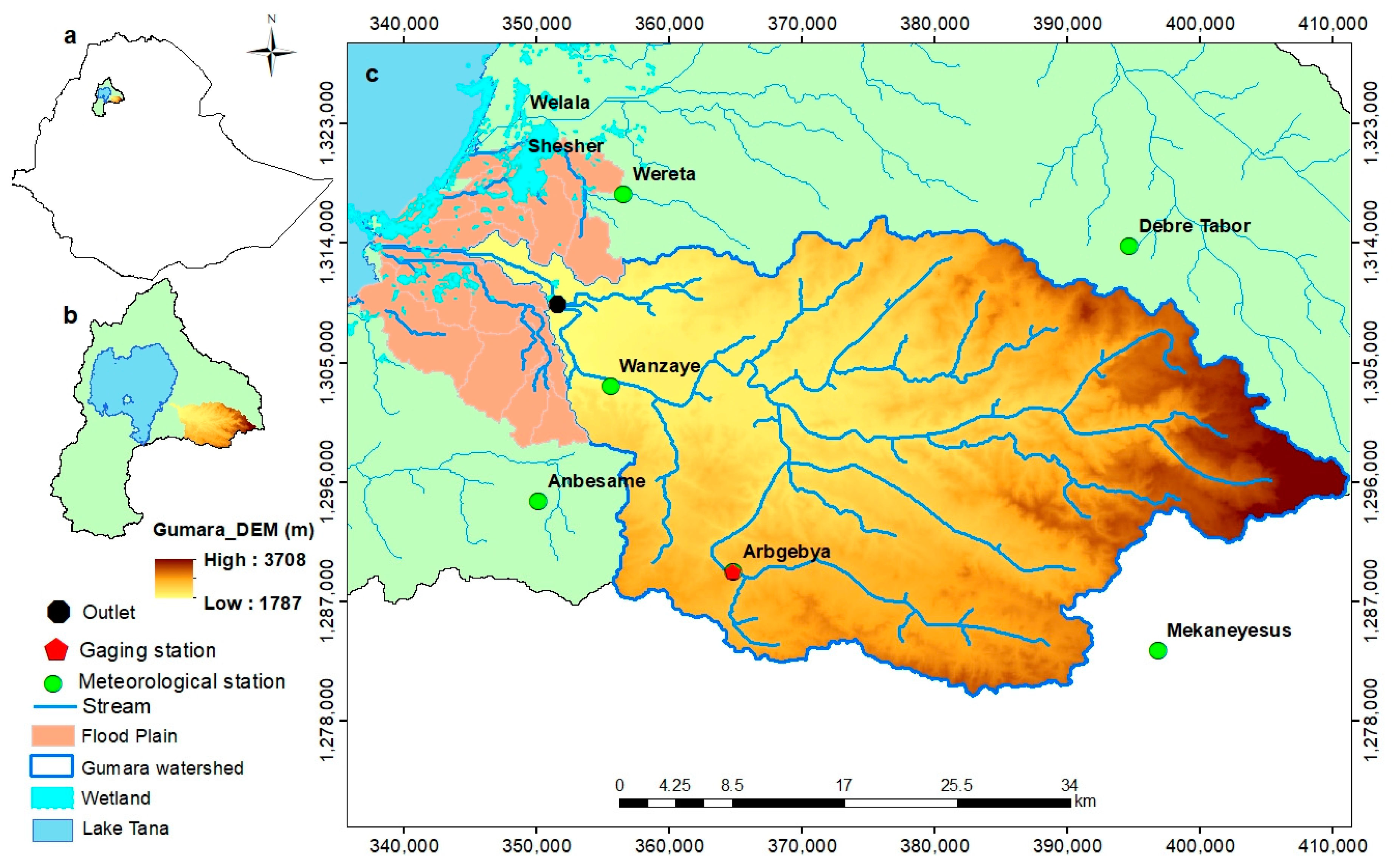
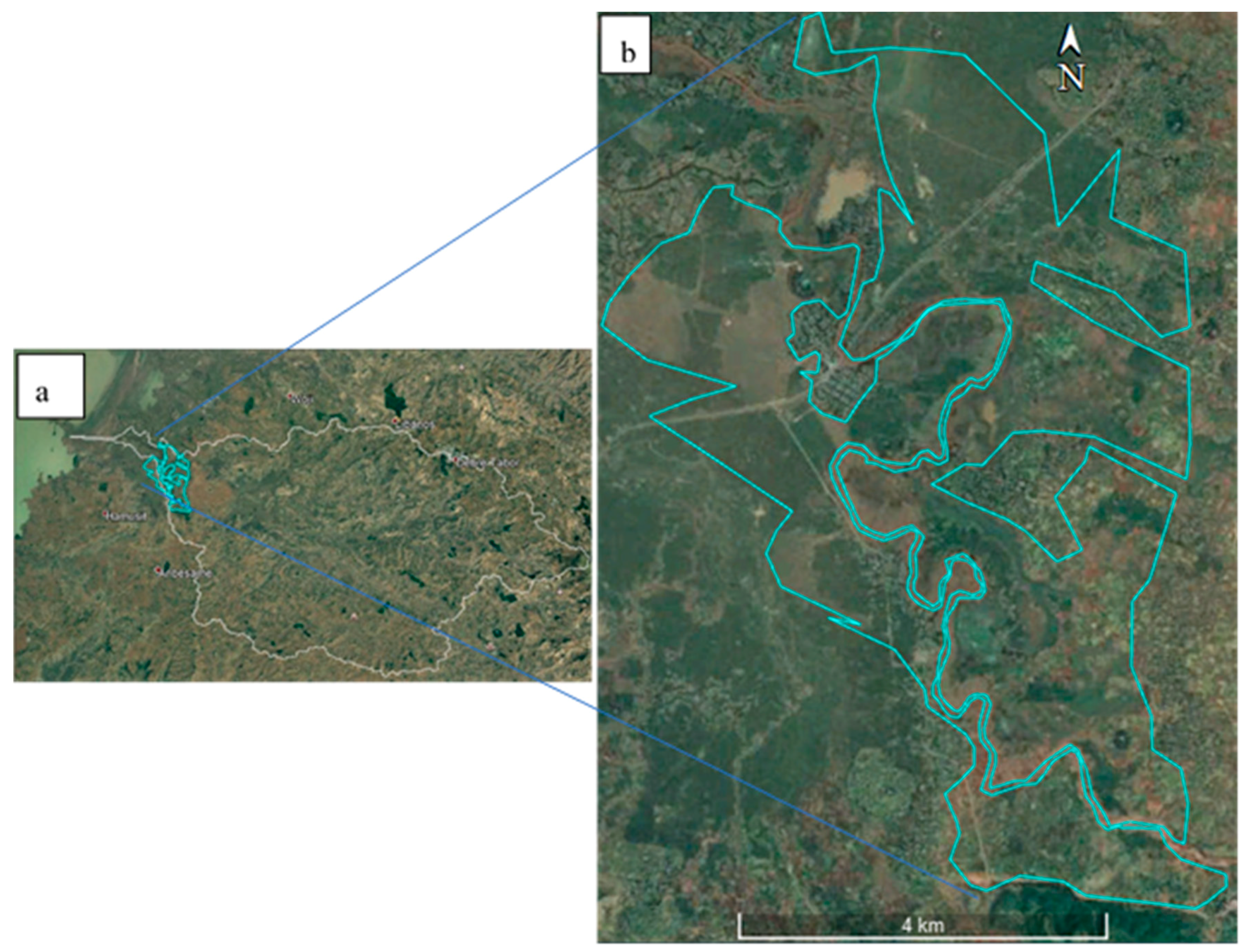
2.1. Study Area Description

The Gumara River originates in the afro-alpine vegetation of the Guna mountains above 4000 m.a.s.l. and flows to Lake Tana at 1784 m.a.s.l. (Figure 2). Gumara River catchment is 1376 km2 and is part of the larger Lake Tana basin. The climate of the area is largely controlled by the movement of the inter-tropical convergence zone (ITCZ), which results in a single rainy season between June and September [26]. The mean annual rainfall over the catchment is 1326 mm year−1. The rivers, before draining to the lake, feed the Welala and Shesher wetlands, which together, cover an area of approximately 8.0 km2 [27,28]. The flood regime of the wetlands is affected by the abstraction and diking of the Gumara River. Moreover, the wetlands are being encroached by cultivation.
Gumara River is ecologically important as it is the migration habitat of fish of the genus Labeobarbus of the cyprinid family [29,30,31,32]. Fifteen unique species of Labeobarbus inhabit the lake [29]. In addition, twelve globally threatened bird species have been identified in Lake Tana and its associated wetlands [33]. Most of the species are recorded in the Shesher and Welala wetlands (Figure 2), which are part of the UNESCO Biosphere reserve areas [34].

2.2. Data Collection

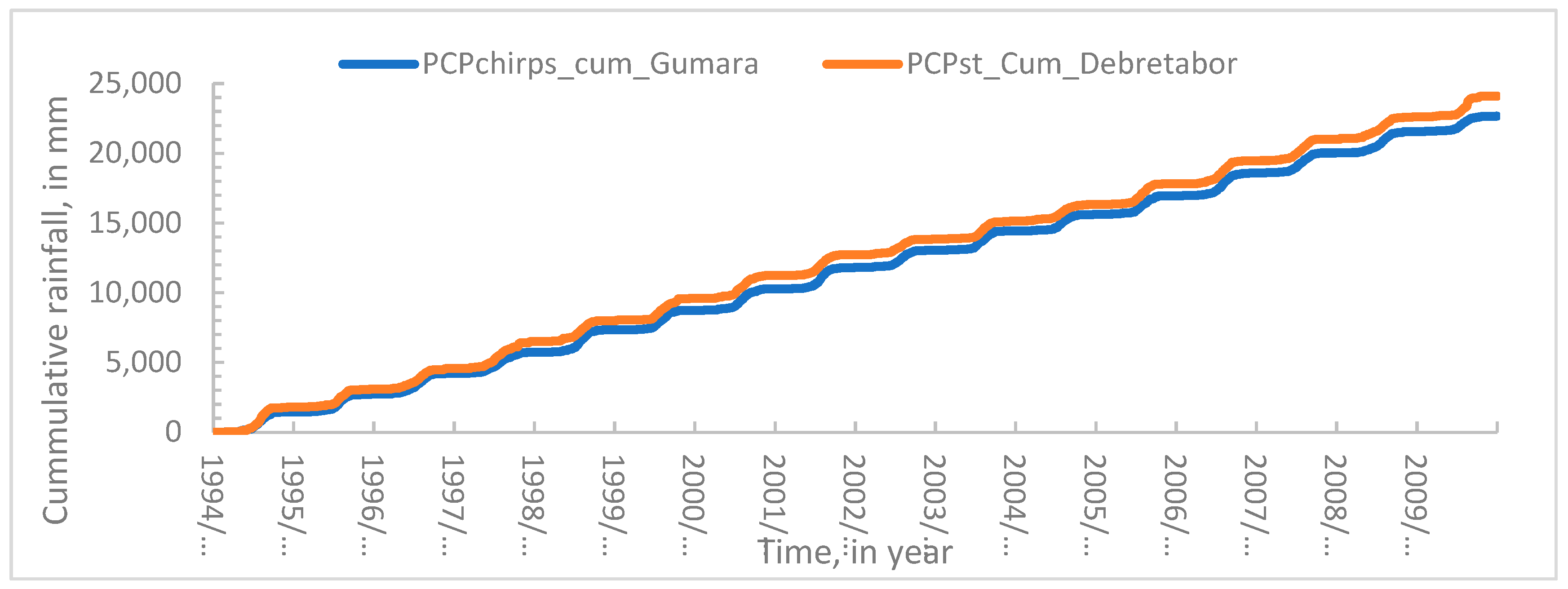
2.2.1. Precipitation

Daily precipitation of the Debretabor, Arb-Gebeya, Mekaneyesus, Wanzaye and Anbessame stations was obtained from the Ethiopian Meteorological Agency (EMA). The dataset was not up to date and complete for all stations. Hence, remote sensing precipitation data of the “Climate Hazards Group InfraRed Precipitation with Station Data” (CHIRPS) with 0.05 arc degree resolution were downloaded for the period from 1 January 1981 to 30 September 2019 from Google Earth Engine; cloud computing platform [35]. CHIRPS was chosen because it has daily data for a long record with the best resolution and performance for this location [35].

2.2.2. Stream Flow

The hydrology was characterized for the entire Gumara catchment using the lower gaging station—No. 111006 (see ‘outlet’ in Figure 2). Flow data for the station were obtained from the Ministry of Water, Irrigation and Electric (MoWIE) from 1960 to 2018. There are large gaps in data for the first 13 years (full years in 1963, and 1967 to 1972), for 5 months in 2015 and for 6 months in 2018. From the total 21,535 days, 3132 (14.5%) were missing. As the annual gaps are too large to fill, we used data from 1973 to 2018.

2.3. Literature Review, Field Observation and Discussions

Literature on fishery and related activities were reviewed. A reconnaissance survey of Gumara catchment and associated wetlands was undertaken and farming communities were questioned on their understanding of flow characteristics and how their livelihoods were connected with the river ecosystem, including pump irrigation, sand mining, vegetation expansion and others.

2.4. Data Analysis

2.4.1. Precipitation and Evapotranspiration Analysis

Areal rainfall of Gumara was estimated from Satellite data of CHIRPS. The performance of CHIRPS was checked by a Pearson correlation test with the available observed data of individual stations around Gumara. Annual, decadal and cumulative rainfall of different durations were calculated using MS EXCEL. The Pearson correlation test was used to visualize the relation of flow and rainfall and Mann–Kendall trend tests were used for trends in rainfall and were performed in SPSS 20, EXCEL and XLstat [36,37]. Cumulative rainfall for generating 20 mm of cumulative direct runoff after the end of the dry season was calculated for trend analysis. In addition, the evapotranspiration over the Gumara catchment was calculated. A synoptic station close to the catchment did not exist to calculate the evapotranspiration from the meteorological data; hence, satellite data of “MOD16A2.006: Terra Net Evapotranspiration 8-Day Global 500 m” was used for the estimate [38].

2.4.2. Flow Analysis Using IHA Software

River flow statistics, components and indices were analyzed using IHA software version 7.1 [39] (The software is developed by the Nature conservacy, Virginia, VA, USA). Setting up and completing an analysis in the IHA involved the use of hydrologic data as input, deciding analysis years and environmental flow component (EFC) thresholds, and water year starting Julian date [39]. Hydrological data from 1973 to 2018 were imported in CSV file format and saved as internal hydrologic file. A project was then created, linked to a single hydrologic data file and used to create and run multiple analysis. The Gumara flow data were not normally distributed (Figure 3) and hence, the non-parametric analysis like medians and coefficient of dispersion were used. The water year was set to start on January 1 and to end on December 31, which is suitable for Gumara River condition.
The IHA calculated parameters for five different types of EFCs which are ecologically relevant: extreme low flows, low flows, high flow pulses, small floods, and large floods. This delineation of EFCs is based on the definition given in the software [1,39]. Low flows are calculated from minimum flows within a year [1,39]. Extreme low flows are taken below the 10th percentile flow.
High-flow pulse is calculated as flow between base flow and bankfull discharge, i.e., including any water rises that do not overtop the channel banks. Small floods include all river rises that overtop the main channel but do not include more extreme and less frequent floods (i.e., below 2-year return period). Large floods are flows calculated as above the 10-year return period, which can inundate distant places from riverbanks, such as lagoons and floodplain wetlands.

2.4.3. Environmental Flow Components Threshold Values Setting

A cumulative distribution function (CDF) curve, flood frequency (FF) curves and stage-discharge (rating) curve were used in setting the EFC threshold values to be input in the IHA software (Figure 3). The CDF curve ensured the non-normality of the data indicating that non-parametric analyses need to be conducted. First, the large flood was found from the 10-year return period of the flood frequency curve; it is 483 m3 s−1 which is the 99.93th percentile in the CDF curve.
The bankfull discharge was estimated using the stage-discharge method [40]. The Bankfull stage was measured and found to be 5.6 m in March 2019.
The stage–discharge curve was developed recently as the bed level increase at the gaging station annually and the offset, h0 changed in time. To do this, h0 was calculated first from the rating curve (Equation (1)) with measured discharge Q and stage height h for streamflow record from February 1990 to March 2018 containing 52 readings. Secondly, the best fitting curve was found through the 52 h0 values [41]. By trial and error, the parameters in Equation (1) were changed until a best fit was obtained. The offset is given in Equation (2):
Q = 11.5 ( h h 0 ) 1.9
The best fit (R2 = 0.93) for the offset, h0 in m was found as
h 0 = 0.0002 ( t 1990 ) 3 + 0.0049 ( t 1990 ) 2 + 0.0748 ( t 1990 ) 0.0819
where t is the year.
The offset, h0 for years before 1990 was estimated using a linear interpolation applied assuming zero in the beginning (1973) and the h0 value calculated for 1990 in Equation (2). Hence, the flow data from the ministry was recalculated for the new h0. Then, the calculated bankfull discharge for 5.6 m stage was found to be 294 m3 s−1 or 97.5% from CDF, which is the maximum for high flow pulse and the starting threshold for small floods. The low flow was found to be 4.8 m3 s−1 (28%) and the maximum extreme low flow was taken as the 10% flow, 0.17 m3 s−1.

2.4.4. Flow Components and Needs

As a complimentary analysis to IHA, ecologically relevant flows from percentiles of the historical daily flows were analyzed seasonally using the approach of DePhilip and Moberg [42]. Overlaying key life history requirements for each group on representative hydrographs for each habitat type, relationships between species groups and seasonal and inter-annual stream flow patterns were explained in terms of flow needs by season. Thresholds were selected to approximate different ecologically relevant flows; Q5–Q10 corresponds to flood levels, Q10–Q75 represents high flows, Q75–Q95 represents low flows, and Q95–Q100 represent the extreme low flows at the site [42]. All daily data of the 46 years were arranged in descending order and their percentiles/exceedance calculated and mapped in Excel where the 5th, 10th, 75th and 95th percentile values are linear interpolations.

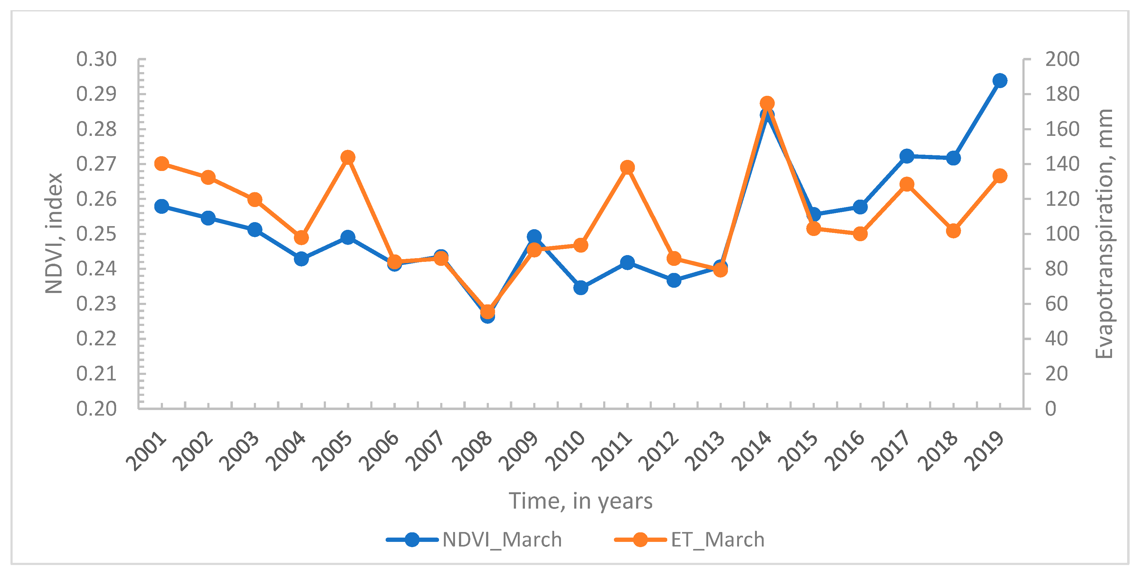
2.4.5. Irrigation Area Mapping and NDVI Analysis

Irrigation practices, sand mining and other economic activities were analyzed using the information obtained from farmers’ discussion and field ground truth data collection using GPS and mapping aided by Google Earth. Discussion with farmers was organized by the local agriculture office experts. A focus group discussion was undertaken for each irrigation and sand mining work. Five farmers who initially started irrigation and 10 individuals who were collecting sand were contacted for discussion using a prepared checklist. The vegetation conditions in the catchment area were also analyzed. Normalized difference vegetation index (NDVI) from MODIS satellite data was calculated in google earth engine, cloud computing platform, to link the impact of vegetation cover change on both low- and high-flow trend.

3. Results and Discussion
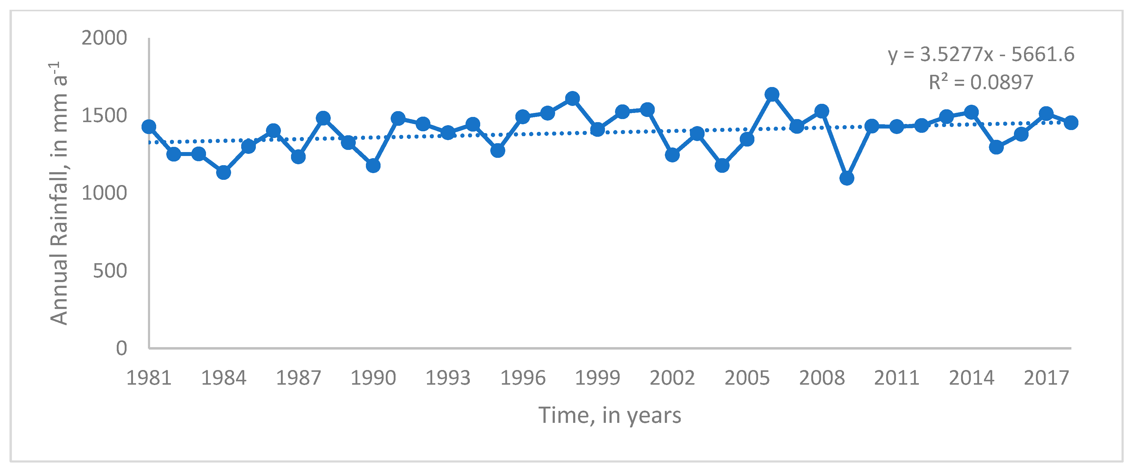
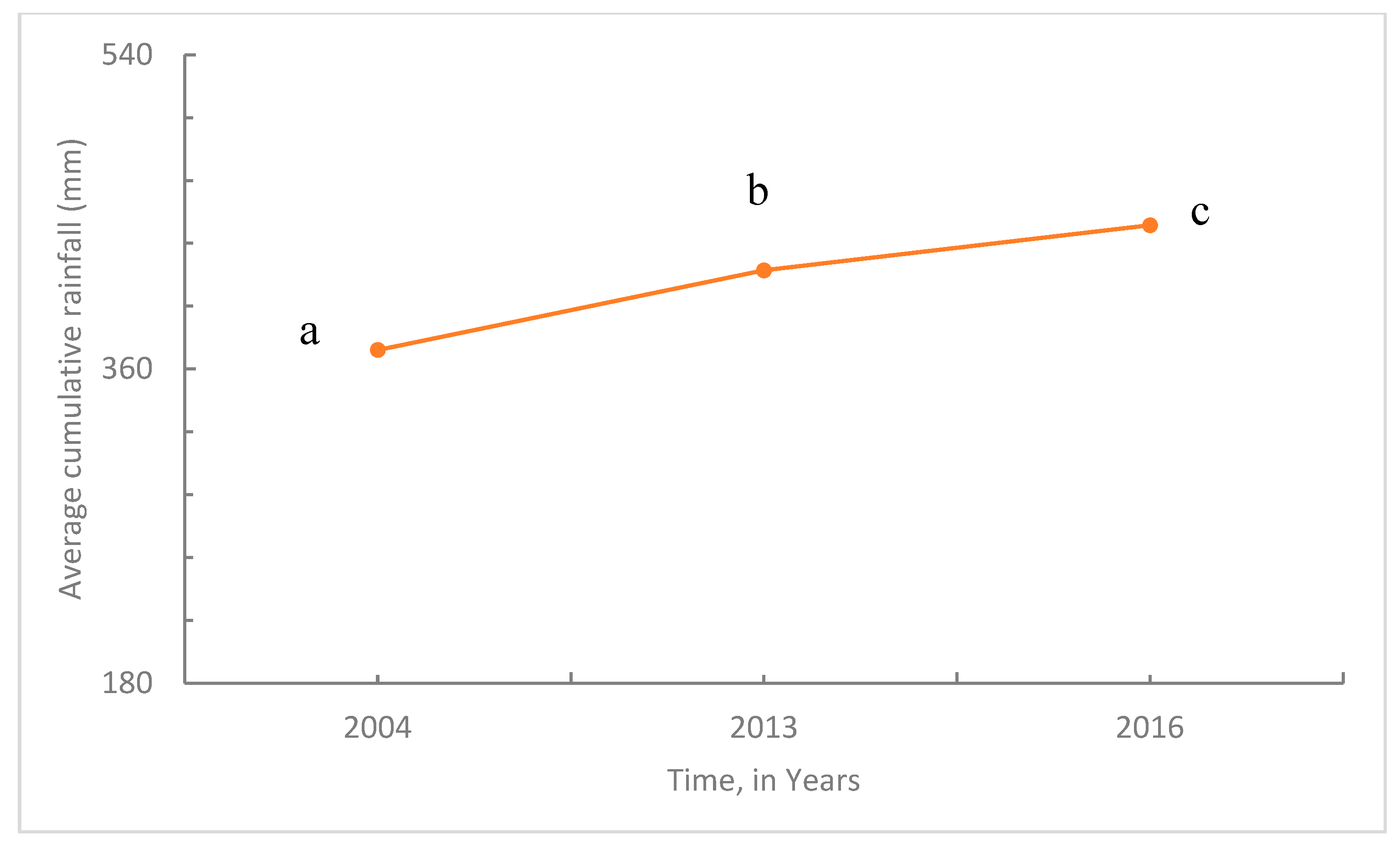
3.1. Precipitation

Data performance from CHRIPS checked by the Pearson’s correlation test with the observed data in SPSS was found to be a correlation coefficient of 0.51 for Debretabor station and a correlation coefficient of 0.44 for Wanzaye station, significant at a 0.01 level (Figure 4). The correlation of the precipitation (PCP) and flow data of Gumara also tested with Pearson correlation test in SPSS and was found to have an r of 0.49; correlation significant at a 0.01 level. The annual precipitation trend of Gumara catchment from the areal estimate for the whole dataset showed a slight increase (Figure 5). The annual PCP trend tested with Mann–Kendal’s test was found to be significant at the 0.05 level.

3.2. Flow Indices

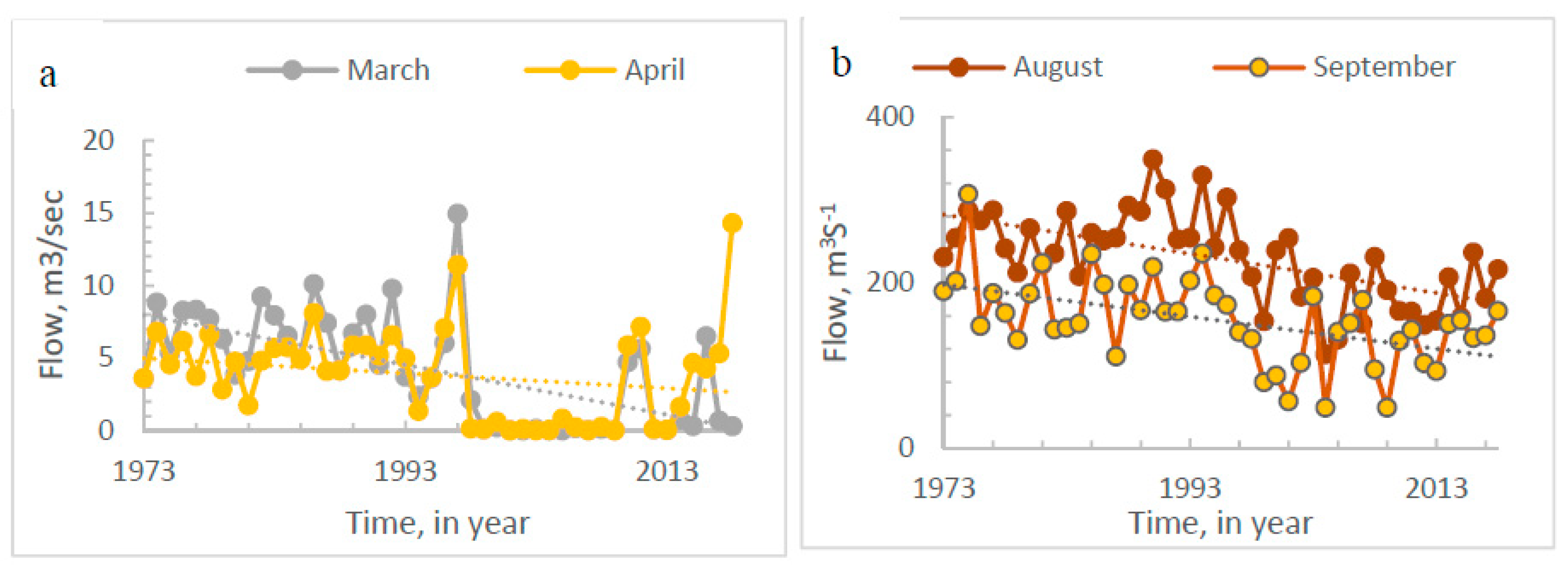
3.2.1. Monthly Flows

The monthly flow analysis indicated that low flow occurs from December to June, the lowest being in March, with a median flow of 4.0 m3 s−1 and a standard error (SE) 0.55 and high flows occur from July to November; the highest being in August, with a median flow of 236 m3 s−1 with a standard deviation of 8 m3 s−1 (Table 1 and Figure 6). A high coefficient of dispersion (COD) was found from November to May during the dry season (winter and spring); and a low COD was observed from June to October during the wet season (summer and autumn).
All monthly flows have a decreasing trend (Figure 6). Flows in the dry season in March and April, decreased in time likely due to pump irrigation and the expansion of eucalyptus trees.

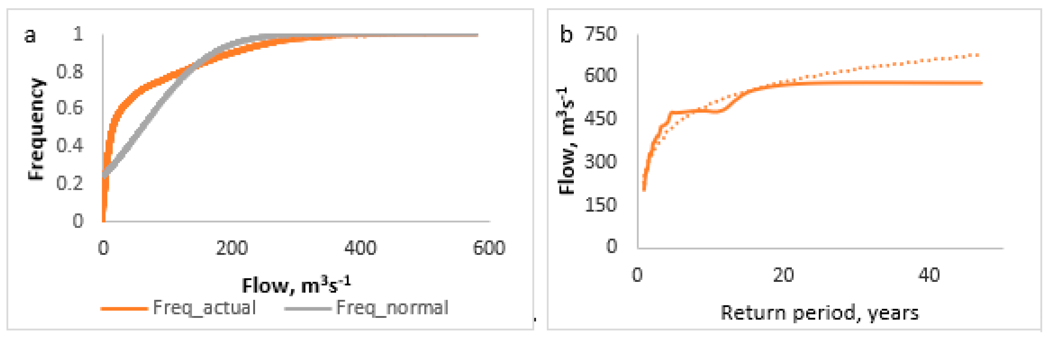
3.2.2. Low and High Flows

Low Flow

The Mann–Kendall trend test indicated that the 1-Day and 90-Day low flow decreased significantly over the study period at p = 0.01. Quantitatively, 1-Day low flow decreased from 1.55 m3 s−1 in 1973 to 0.16 m3 s−1 in 2018 and 90-Day (seasonal) low flow decreased from 4.88 m3 s−1 in 1973 to 2.04 m3 s−1 in 2018. The decrease in low flow after 1997 was verified in the discussion with farmers and district experts living and working in the study area. According to the discussants, pump irrigation started in 1997 using the pumps supported by German International Cooperation (GIZ). In the first year, pump irrigation was started by 25 farmers who were cultivating maize, then it reached maximum to all households in 2005. The delineation using Google Earth indicated that irrigated area was 29 km2 in 2019 (Figure 7). The average historical low flow before 1997 was 3.03 m3 s−1 or 3,141,504 m3 of water per year. The net irrigable area of the lower Gumara is 15.25 km2, distributed 6 km2 Onion, 0.2 km2 Tomato, 0.82 km2 Garlic, 0.16 km2 Pepper, 2.0 km2 Tef, 6 km2 Maize, and 0.07 km2 Lentil (Annual report 2018/19, Dera District Agriculture Office). The irrigation water requirement of Onion is 288,300 m3 km−2, Tomato 168,900 m3 km−2, Pepper 127,100 m3 km−2, Garlic 144,200 m3 km−2, Tef 84,150 m3 km−2, Lentil 308,300 m3 km−2, and Maize 167,450 m3 km−2 [43]. This amounts to a demand of 3,096,741 m3 of water per year for 15.25 km2, which is 99% of the value of the historical low flows before 1997.
There was an abrupt decrease of low flow in 1997 which remained at a bare minimum onwards. The coefficient of dispersion (COD) values are greater for all duration of flow, indicating greater variability in low flow (Table 2 and Figure 8). The mean decadal low flows were 3.02, 3.19, 1.96, 0.002, and 0.029 m3 s−1 for 1973–1980, 1981–1990, 1991–2000, 2001–2010 and 2011–2018, respectively (Table 3).The extreme decrease in low flow components impacts the predators of fish, reducing their mobility and ability to access prey concentrated in smaller pools.

High Flow

The maximum flows, similarly to the low flows, decreased over the time periods: 1-Day r2 of 0.53 with significant trend at p = 0.01 with Mann–Kendall’s test and 90-Day r2 of 0.32 (p = 0.01). Quantitatively, 1-Day high flow decreased from 335 m3 s−1 in 1973 to 266 m3 s−1 in 2018 and 90-Day (seasonal) high flow decreased from 188 m3 s−1 in 1973 to 185 m3 s−1 in 2018. The 1-Day maximum is a good indicator for large flood decrease as it indicates individual peaks rather than averages as the other durations do (Table 2 and Figure 8). The mean decadal high flow ranged from 432 m3 s−1 to 261 m3 s−1 between 1973 and 1980 and 2001 and 2010, respectively (Table 3).
From these results, we infer that the river is becoming disconnected earlier from the floodplain wetlands because of a decrease in “ecologically relevant” large floods. As studies indicated, this has an impact on fish breeding habitat shrinkage in a short period of time [44]. A decline in juvenile labeobarb abundance in the pool habitats of Gumara River occurred because of excess irrigation water abstraction, especially in the dry season months of March to May [44]. In addition, several studies found that in recent years, fish stocks declined rapidly, especially commercially important fish species like Labeobarbus’ which are migratory fishes requiring wetland habitats for breeding [23,32,45].
We inferred that the decrease in large flood and in low flows during dry season is attributed to unmanaged pump irrigation, the expansion of plantations and soil conservation works being undertaken since 2010 through government mass mobilization program. This agrees with the other studies in lake Tana Basin [46]. In addition, a study on the hydrological impact of a Eucalyptus plantation found that the cumulative rainfall required to generate 3 mm runoff was higher after a threefold expansion of the plantation area [47].
The normalized difference vegetation index (NDVI) for Gumara catchment was checked by extracting NDVI data in Google Earth engine, cloud computing platform, and showed a significant increasing trend at a 0.05 level (Figure 9). An increase in vegetation is expected to decrease (direct) runoff due to increasing evapotranspiration.
Therefore, using the satellite image data of MODIS, the dry season, the month of March, evapotranspiration over the Gumara was extracted and found to be increasing between 2001 and 2019 (Figure 9). The correlation of evapotranspiration with NDVI was 0.64 with Pearson’s correlation test; significant at the 0.01 level. The evapotranspiration is in line with the vegetation increase in the Gumara Catchment. An increase in vegetation has increased the evapotranspiration, which, in turn, increased the amount of infiltration water need to saturate soils before runoff generation. This suggests that the hydrological process is highly influenced by tree plantations [47,48].
Research has shown that in the Ethiopian highlands where saturation excess runoff dominates, daily discharge is a function of daily amount of rainfall, not of the rainfall intensity [48,49,50]. For watersheds to start generating surface runoff after the dry monsoon phase, the soil needs to become saturated [48,49,50]. We divided the study period into three blocks before catchment management interventions, including vegetation expansions (1998 to 2011), during interventions (2012 to 2014) and after soil and water conservation and vegetation expansions (2015 to 2018). The average cumulative rainfall required for a 20 mm runoff depth increased from 371 mm in the first period before intervention to 442 mm after interventions (Figure 10). The result agrees with the finding of another recent study from the Ethiopian Highlands [47].

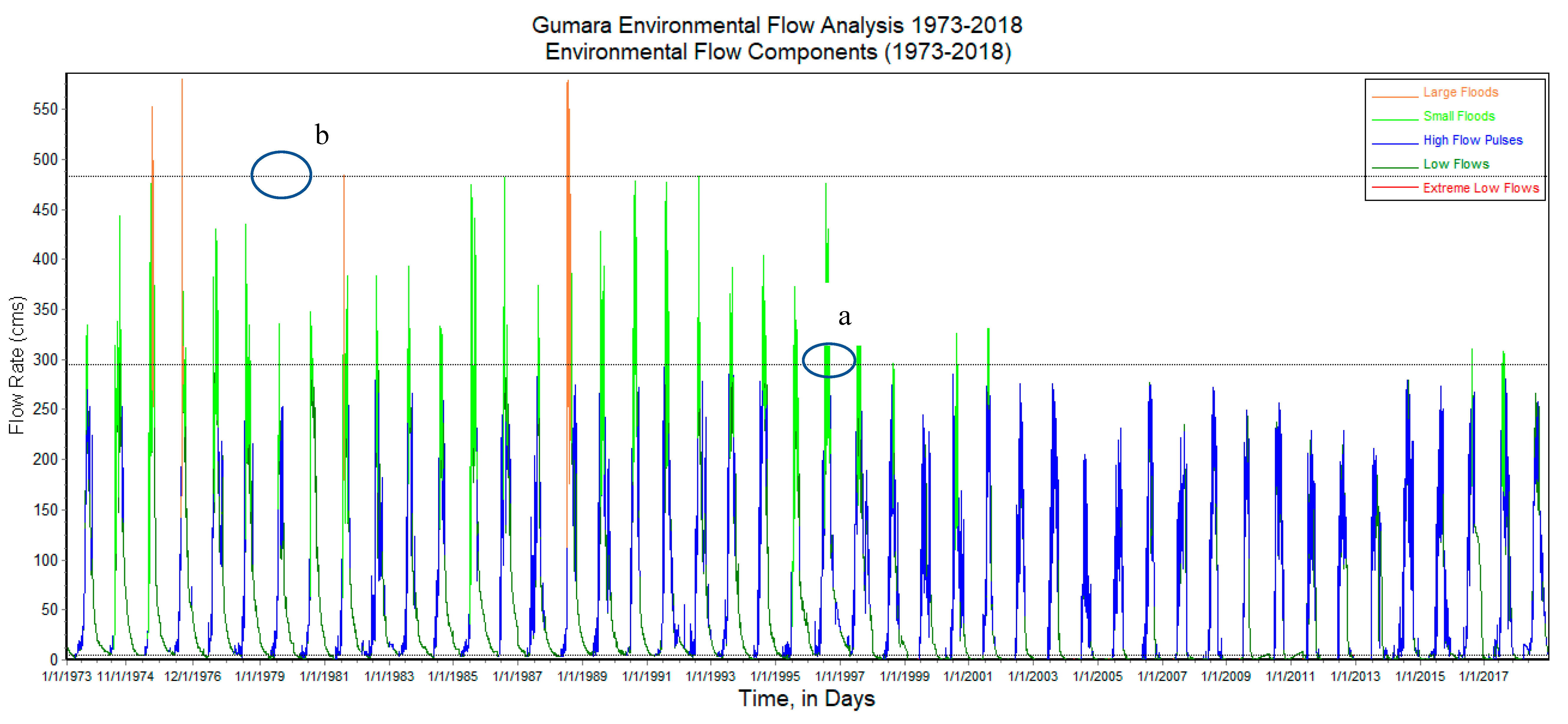
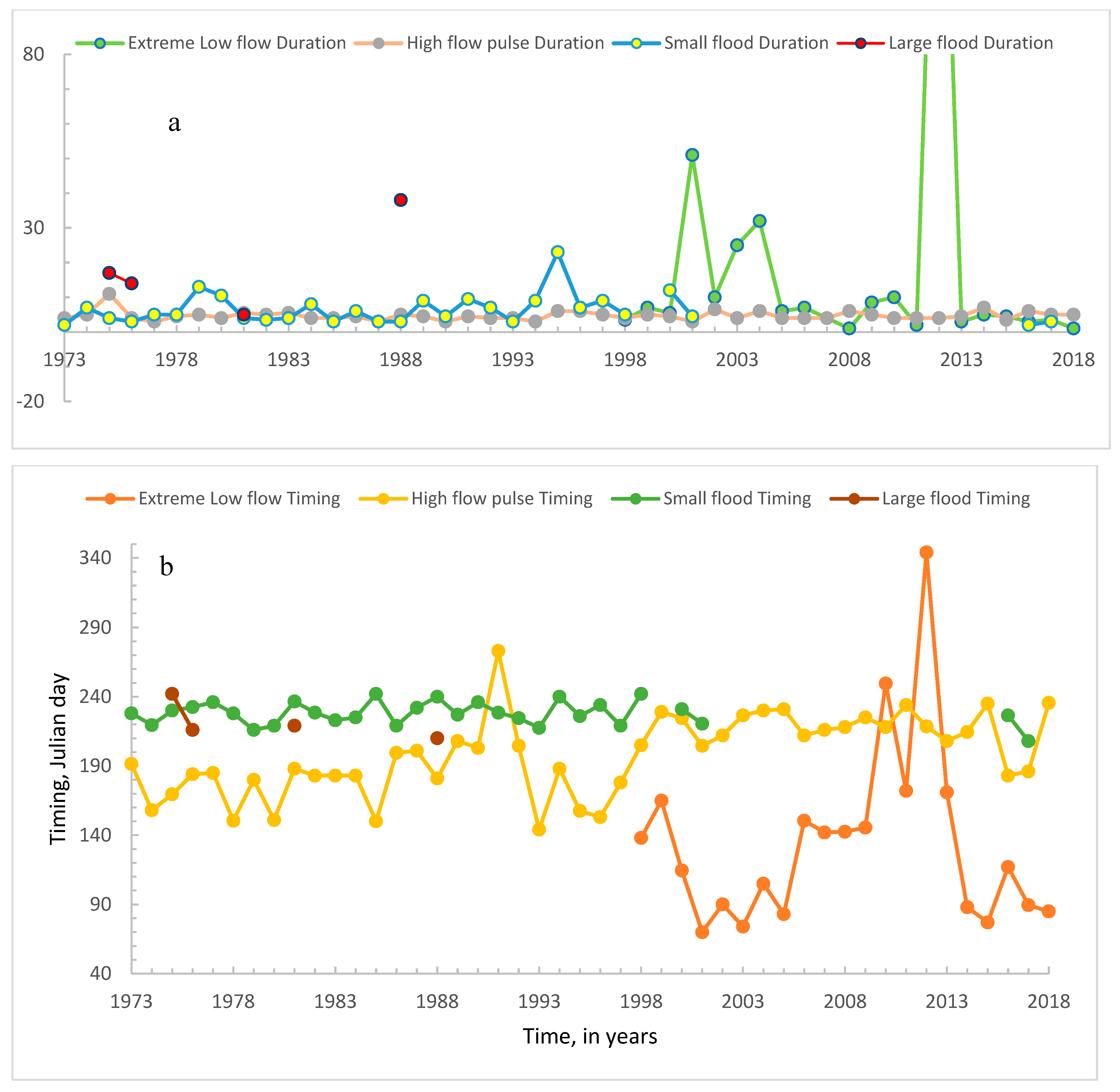
3.3. Environmental Flow Components (EFC), Durations and Timing

Environmental Flow Components

The EFC analysis found four large floods during the last 50 years, i.e., 1975, 1976, 1981 and 1988 (Figure 11). Interestingly, no large flood was recorded after 1989 and small floods exhibited a decrease after 1997. This has a similar interpretation with low- and high-flow condition. This results in an early disconnection of floodplain wetlands from the river and the lake, which impacts fish migration, spawning/breeding, and the growth period for juveniles. High-flow pulse increased and shows a nearly uniform magnitude in the last decades. On the other hand, extreme low flow and low flow decreased and could have an impact on predator-prey relationships as species are concentrated in smaller pools (Figure 11).

Flow Duration and Timing of Environmental Flow Components

All environmental flow components showed increasing duration except for high flow pulses (Figure 12). Extreme low flow showed increase in trend where low flow in other ways decreased in recent years. According to the flow components analysis, large and small floods were not available after 1988 and 2001 respectively. High-flow pulse, which occurs at the beginning of the wet season, is almost undisturbed, which can give fish and other aquatic animals increased access to upstream areas. This flow component is not enough for complete fish reproduction, which need spawning and a growth period in the river and flood plain wetlands provided by small and large floods.
The timing (the Julian day) of small flood occurrence is stable between 214 and 244 with a median of 228 and a COD of 0.039 but it is interrupted after 2001. Other environmental flow components are highly variable; for example, high-flow pulse moved from 194 Julian day in 1973 to about 230 Julian day in 2018, which is almost a month delay (Figure 12). This can cause a disruption of the reproduction cycle of fish and other aquatic animals which live both in the lake and river. High-flow pulses are a signal for these species to begin migrating into rivers to reach floodplain spawning areas.

3.4. Flow Components and Needs

The seasons considered in northwest Ethiopia are: the rainy season (Summer)—June, July and August; the beginning of the dry season (Autumn)—September, October and November; the dry season (Winter)—December, January and February; and end of dry season (Spring)—March, April and May. Figure 13 depicts the percentile flows for individual days of the calendar year over the duration of the discharge record for the bridge gauging station.
To relate flow regimes to ecological responses, we looked at fish spawning migration and reproduction with the percentile flows of Gumara River classified into different ecologically relevant flow components (Figure 13). This is in line with another similar study [42]. The definition of life histories of indicator fish species sensitive to hydrologic alterations in the study area is based on the literature [22,30,31,32,45,51,52,53,54,55,56] (Table 4). An overlay graph, Figure 13, depicts periods of fish spawning migration and reproduction with the percentile flows of Gumara river classified into different ecologically relevant flow components.
The overlaid graph, Figure 13, shows that spawning migration and reproduction begin in June and July for most fish species. Migration kicks off as freshest water or flow pulses reach the lake; high-flow pulses begin from 4.8 m3 s−1 in June and small floods from 294 m3 s−1 in July (Figure 13). However, some fish species, such as B. humilis and B. tanapelagious, stay in the littoral zone of the lake for reproduction [45].
As studies indicated, among commercially important migratory fishes of Lake Tana like C. gariepinus (cat fish), the major breeding season extends from April to July [51] (Table 4 and Figure 13). C. gariepinus requires the seasonal flow to emigrate from the Lake to the flood plain wetlands of Shesher and Welala via Gumara River to start the spawning. As shown in Figure 11, the high flow pulse (seasonal flow) has been delayed by one-month. This likely leads to a corresponding delay in the beginning of the spawning period of species like C. gariepinus (Figure 13).
This study has comparable results with recent studies globally which developed analytical connections between flow alterations and ecological responses (in testing the ELOHA framework) and suggested restoration possibilities [57,58,59]. Hence, results from this study indicate that the Gumara River and associated wetlands need restoration of ecologically relevant environmental flow components (large flood, small flood, high flow pulse, low flow and extreme low flow) to reverse the deterioration of the aquatic ecosystems in the river-wetland-lake interconnections. This will help to restore the aquatic ecosystem through regulating water resources use and appropriate conservation works in the upper watershed.

4. Conclusions

The results of this study indicate that low- and high-flow regimes of Gumara River have decreased over time. The low flow decrease was abrupt since 1997. Large floods also disappeared since 1988. One-day low flows decreased from 1.55 m3 s−1 in 1973 to 0.16 m3 s−1 in 2018, and 90-Day (seasonal) low flow decreased from 4.88 m3 s−1 in 1973 to 2.04 m3 s−1 in 2018. The decrease in flows in time is attributed to both water abstractions, catchment management interventions and rainfall variability. The cumulative rainfall required to generate runoff has increased over the study years. This flow reduction results in early disconnection of floodplain wetlands from the river, which, in turn, affects the breeding cycle of migratory fish species in the floodplain wetlands. Hence, the results of this study indicate that the Gumara River and associated wetlands need restoration of ecologically relevant flows (large flood, small flood, high-flow pulse, low-flow and extreme low-flow) to reverse the deterioration of the aquatic ecosystems in the river-wetland-lake interconnections. This will help to restore the aquatic ecosystem through regulating water resources use and appropriate conservation work in the upper watershed. The environmental flow management framework developed by NBI and the Ecological limits of hydrologic alteration (ELOHA) have helped to guide the study of the environmental flow components dynamics of the Gumara River. Finally, these results serve as the hydrological foundation for continued studies in the Gumara catchment, with the eventual goal of quantifying environmental flow requirements.

Author Contributions

Conceptualization, W.B.A., S.A.T. and M.E.M.; Data curation, W.B.A.; Formal analysis, W.B.A., S.A.T., T.A.N., D.A.M., M.V.C., K.W. and M.E.M.; Funding acquisition, W.B.A., S.A.T. and K.W.; Investigation, W.B.A.; Methodology, W.B.A., S.A.T., M.M.M., A.W. and M.E.M.; Project administration, S.A.T.; Resources, S.A.T., M.M.M., A.W. and K.W.; Supervision, S.A.T., M.M.M., A.W. and M.E.M.; Validation, T.S.S., K.W. and M.E.M.; Writing—original draft, W.B.A.; Writing—review and editing, W.B.A., S.A.T., M.M.M., M.G.D., T.A.N., D.A.M., T.S.S., M.V.C., K.W. and M.E.M. All authors have read and agreed to the published version of the manuscript.

Funding

This research was funded by Amhara Design and Supervision Works Enterprise, Global Minds Fund of Laboratory of Applied Geology and Hydrogeology in Ghent University and the PIRE project: “Taming Water in Ethiopia—An Interdisciplinary Approach to Improve Human Security in a Water-Dependent Emerging Region” supported by the National Science Foundation (NSF) under Grant No. 154587.4.

Acknowledgments

The flow data were obtained from Ministry of Water, Irrigation and Electric. Abbay basin Authority provided stage and discharge data. The authors acknowledged financial and technical support by the International Center for Tropical Agriculture (CIAT), the USAID-funded Africa RISING program, and the Water, Land and Ecosystems (WLE) Program of the CGIAR. The authors acknowledged the three anonymous reviewers and Professor Jan Nyssen who have provided comments on the manuscript.

Conflicts of Interest

The authors declare that there is no conflict of interest.

References

  1. Richter, B.D.; Baumgartner, J.V.; Powell, J.; Braun, D.P. A method for assessing hydrologic alteration within ecosystems. Conserv. Biol. 1996, 10, 1163–1174. [Google Scholar] [CrossRef] [Green Version]
  2. McClain, M.E. Balancing water resources development and environmental sustainability in Africa: A review of recent research findings and applications. Ambio 2013, 42, 549–565. [Google Scholar] [CrossRef] [PubMed] [Green Version]
  3. Pahl-Wostl, C.; Arthington, A.; Bogardi, J.; Bunn, S.; Hoff, H.; Lebel, L.; Nikitina, E.; Palmer, M.; Poff, L.N.; Richards, K.; et al. Environmental flows and water governance: Managing sustainable water uses. Curr. Opin. Environ. Sustain. 2013, 5, 341–351. [Google Scholar] [CrossRef]
  4. Reitberger, B.; McCartney, M. Concepts of Environmental Flow Assessment and Challenges in the Blue Nile Basin, Ethiopia, in Nile River Basin; Springer: Berlin/Heidelberg, Germany, 2011; pp. 337–358. [Google Scholar]
  5. Arthington, A.H.; Naiman, R.J.; McClain, M.E.; Nilsson, C. Preserving the biodiversity and ecological services of rivers: New challenges and research opportunities. Freshw. Biol. 2010, 55, 1–16. [Google Scholar] [CrossRef] [Green Version]
  6. Caissie, D.; El-Jabi, N.; Hébert, C. Comparison of hydrologically based instream flow methods using a resampling technique. Can. J. Civ. Eng. 2007, 34, 66–74. [Google Scholar] [CrossRef]
  7. Hughes, D.A.; Hannart, P. A desktop model used to provide an initial estimate of the ecological instream flow requirements of rivers in South Africa. J. Hydrol. 2003, 270, 167–181. [Google Scholar] [CrossRef]
  8. Tharme, R.E. A global perspective on environmental flow assessment: Emerging trends in the development and application of environmental flow methodologies for rivers. River Res. Appl. 2003, 19, 397–441. [Google Scholar] [CrossRef]
  9. Hughes, D. Providing hydrological information and data analysis tools for the determination of ecological instream flow requirements for South African rivers. J. Hydrol. 2001, 241, 140–151. [Google Scholar] [CrossRef]
  10. King, J.M.; Tharme, R.E.; De Villiers, M. Environmental Flow Assessments for Rivers: Manual for the Building Block Methodology; Water Research Commission: Pretoria, South Africa, 2000. [Google Scholar]
  11. Zalewski, M.; Negussie, Y.Z.; Urbaniak, M. Ecohydrology for Ethiopia—Regulation of water biota interactions for sustainable water resources and ecosystem services for societies. Ecohydrol. Hydrobiol. 2010, 10, 101–106. [Google Scholar] [CrossRef] [Green Version]
  12. Poff, N.L.; Richter, B.D.; Arthington, A.H.; Bunn, S.E.; Naiman, R.J.; Kendy, E.; Acreman, M.; Apse, C.; Bledsoe, B.P.; Freeman, M.C.; et al. The ecological limits of hydrologic alteration (ELOHA): A new framework for developing regional environmental flow standards. Freshw. Biol. 2010, 55, 147–170. [Google Scholar] [CrossRef] [Green Version]
  13. Poff, N.L.; Allan, J.D. Functional organization of stream fish assemblages in relation to hydrological variability. Ecology 1995, 76, 606–627. [Google Scholar] [CrossRef]
  14. NBI, Preparation of NBI Guidance Document on Environmental Flows: Nile E-Flows Framework Technical Implementation Manual; HYDROC GmbH: Siegum, Germany, 2016.
  15. Alemayehu, T.; McCartney, M.; Kebede, S. The water resource implications of planned development in the Lake Tana catchment, Ethiopia. Ecohydrol. Hydrobiol. 2010, 10, 211–221. [Google Scholar] [CrossRef]
  16. Awulachew, S.B. Water Resources and Irrigation Development in Ethiopia; Iwmi: Colombo, Sri Lanka, 2007; Volume 123. [Google Scholar]
  17. Setegn, S.G.; Rayner, D.; Melesse, A.M.; Dargahi, B.; Srinivasan, R. Impact of climate change on the hydroclimatology of Lake Tana Basin, Ethiopia. Water Resour. Res. 2011, 47. [Google Scholar] [CrossRef]
  18. Belete, M.A. Modeling and Analysis of Lake Tana Sub Basin Water Resources Systems, Ethiopia; Univ. Agrar-und Umweltwiss: Rostock, Germany, 2014. [Google Scholar]
  19. Duan, W.; He, B.; Takara, K.; Luo, P.; Nover, D.; Hu, M. Impacts of climate change on the hydro-climatology of the upper Ishikari river basin, Japan. Environ. Earth Sci. 2017, 76, 490. [Google Scholar] [CrossRef]
  20. Zou, S.; Jilili, A.; Duan, W.; De Maeyer, P.; Van De Voorde, T. Human and Natural Impacts on the Water Resources in the Syr Darya River Basin, Central Asia. Sustainability 2019, 11, 3084. [Google Scholar] [CrossRef] [Green Version]
  21. Abebe, W.B.; Douven, W.J.A.M.; McCartney, M.; Leentvaar, J. EIA Implementation and Follow Up: A Case Study of Koga Irrigation and Watershed Management Project ETHIOPIA; Unesco-IHE: Delft, The Netherlands, 2007. [Google Scholar]
  22. Anteneh, W.; Getahun, A.; Dejen, E.; Sibbing, F.A.; Nagelkerke, L.A.J.; De Graaf, M.; Wudneh, T.; Vijverberg, J.; Palstra, A.P. Spawning migrations of the endemic Labeobarbus (Cyprinidae, Teleostei) species of Lake Tana, Ethiopia: Status and threats. J. Fish Biol. 2012, 81, 750–765. [Google Scholar] [CrossRef] [PubMed]
  23. Dejen, E.; Anteneh, W.; Vijverberg, J. The decline of The Lake Tana (Ethiopia) fisheries: Causes and possible solutions. Land Degrad. Dev. 2017, 28, 1842–1851. [Google Scholar] [CrossRef] [Green Version]
  24. Duan, W.; He, B.; Nover, D.; Yang, G.; Chen, W.; Meng, H.; Zou, S.; Liu, C. Water quality assessment and pollution source identification of the eastern Poyang Lake Basin using multivariate statistical methods. Sustainability 2016, 8, 133. [Google Scholar] [CrossRef] [Green Version]
  25. Dagnew, D.C.; Guzman, C.D.; Zegeye, A.D.; Akal, A.T.; Moges, M.A.; Tebebu, T.Y.; Mekuria, W.; Ayana, E.K.; Tilahun, S.A.; Steenhuis, T.S. Sediment loss patterns in the sub-humid ethiopian highlands. Land Degrad. Dev. 2017, 28, 1795–1805. [Google Scholar] [CrossRef]
  26. Abebe, W.B.; GMichael, T.; Leggesse, E.S.; Beyene, B.S.; Nigate, F. Climate of Lake Tana Basin. In Social and Ecological System Dynamics; Springer: Berlin/Heidelberg, Germany, 2017; pp. 51–58. [Google Scholar]
  27. Atnafu, N.; Dejen, E.; Vijverberg, J. Assessment of the Ecological Status and Threats of Welala and Shesher Wetlands, Lake Tana Sub-basin (Ethiopia). J. Water Resour. Prot. 2011, 3, 540–547. [Google Scholar] [CrossRef] [Green Version]
  28. Karlberg, L.; Hoff, H.; Amsalu, T.; Andersson, K.; Binnington, T.; Flores-López, F.; de Bruin, A.; Gebrehiwot, S.; Gedif, A.B.; Heide, F.Z.; et al. Tackling complexity: Understanding the food-energy-environment nexus in Ethiopia’s Lake Tana sub-basin. Water Altern. 2015, 8, 710–734. [Google Scholar]
  29. Nagelkerke, L.; Sibbing, F.A. The Barbs of Lake Tana, Ethiopia: Morphological Diversity and Its Implications for Taxonomy, Trophic Resource Partitioning, and Fisheries. Ph.D. Thesis, Wageningen Agricultural University, Wageningen, The Netherlands, 1997. [Google Scholar]
  30. Goshu, G.; Tewabe, D.; Adugna, B.T. Spatial and temporal distribution of commercially important fish species of Lake Tana, Ethiopia. Ecohydrol. Hydrobiol. 2010, 10, 231–240. [Google Scholar] [CrossRef]
  31. Shitaw, T.; Medehin, S.G.; Anteneh, W. Spatio-temporal distribution of Labeobarbus species in Lake Tana. Int. J. Fish. Aquat. Stud. 2018, 6, 562–570. [Google Scholar]
  32. Ameha, A.; Assefa, A. The Fate of The Barbus of Gumara River, Ethiopia. SINET Ethiop. J. Sci. 2002, 25, 1–18. [Google Scholar] [CrossRef] [Green Version]
  33. Aynalem, S.; Bekele, A. Species composition, relative abundance and distribution of bird fauna of riverine and wetland habitats of Infranz and Yiganda at southern tip of Lake Tana, Ethiopia. Trop. Ecol. 2008, 49, 199. [Google Scholar]
  34. Zur Heide, F. Feasibility Study for a Lake Tana Biosphere Reserve, Ethiopia; Bundesamt für Naturschutz, BfN: Bonn, Germany, 2012. [Google Scholar]
  35. Funk, C.; Peterson, P.; Landsfeld, M.; Pedreros, D.; Verdin, J.; Shukla, S.; Husak, G.; Rowland, J.; Harrison, L.; Hoell, A.; et al. The climate hazards infrared precipitation with stations—A new environmental record for monitoring extremes. Sci. Data 2015, 2, 150066. [Google Scholar] [CrossRef] [Green Version]
  36. Kendall, M. Rank Correlation Methods; Charles Griffin: London, UK, 1975. [Google Scholar]
  37. Mann, H.B. Non-parametric tests against trend. Econom. J. Econom. Soc. 1945, 13, 245–259. [Google Scholar]
  38. Running, S.; Mu, Q.; Zhao, M. MOD16A2 MODIS/Terra Net Evapotranspiration 8-Day L4 Global 500 m SIN Grid V006; NASA EOSDIS Land Processes DAAC: Washington, DC, USA, 2017. [Google Scholar]
  39. The Nature Conservancy. Indicators of Hydrologic Alteration Version 7.1 User’s Manual; The Nature Conservancy: Virginia, VA, USA, 2009. [Google Scholar]
  40. Williams, G.P. Bank-full discharge of rivers. Water Resour. Res. 1978, 14, 1141–1154. [Google Scholar] [CrossRef]
  41. Nigatu, T.A.; Zimale, F.A.; Tilahun, S.A.; Abebe, W.B.; Behulu, Y.M.; Tegegn, B.A.; Steenhuis, T.S. Rating Curves for Infrequently Calibrated River Gauging Stations at the Rivers in Lake Tana Basin, Ethiopia. Water 2020, in press. [Google Scholar]
  42. DePhilip, M.; Moberg, T. Ecosystem Flow Recommendations for the Susquehanna River Basin; The Nature Conservancy: Harrisburg, PA, USA, 2010. [Google Scholar]
  43. ADSWE. Upper Rib Large Scale Irrigation Project, Volume IV: Irrigation Agronomy; Amhara National Regional State, Bureau of Water, Irrigation & Energy Development: Bahir Dar, Ethiopia, 2018. [Google Scholar]
  44. Dejen, E.; Vreven, E. Habitat Use and Downstream Migration of 0+ Juveniles of the Migratory Riverine Spawning Labeobarbus Species (Cypriniformes: Cyprinidae) of Lake Tana (Ethiopia). In Proceedings of the Fifth International Conference of the Pan African Fish and Fisheries Association (PAFFA5), Bujumbura, Burundi, 16–20 September 2013. [Google Scholar]
  45. Gebremedhin, S.; Getahun, A.; Anteneh, W.; Bruneel, S.; Goethals, P. A Drivers-Pressure-State-Impact-Responses Framework to Support the Sustainability of Fish and Fisheries in Lake Tana, Ethiopia. Sustainbility 2018, 10, 2957. [Google Scholar] [CrossRef] [Green Version]
  46. Enku, T.; Tadesse, A.; Yilak, D.L.; Gessesse, A.A.; Addisie, M.B.; Abate, M.; Zimale, F.A.; Moges, M.A.; Tilahun, S.A.; Steenhuis, T.S. Biohydrology of low flows in the humid Ethiopian highlands: The Gilgel Abay catchment. Biologia 2014, 69, 1502–1509. [Google Scholar] [CrossRef]
  47. Mhiret, D.A.; Dagnew, D.C.; Alemie, T.C.; Guzman, C.D.; Tilahun, S.A.; Zaitchik, B.F.; Steenhuis, T.S. Impact of Soil Conservation and Eucalyptus on Hydrology and Soil Loss in the Ethiopian Highlands. Water 2019, 11, 2299. [Google Scholar] [CrossRef] [Green Version]
  48. Enku, T.M.; Ayana, A.M.; Tilahun, E.K.; Mengiste, S.A.; Abate, M.; Steenhuis, T.S. Groundwater use of a small eucalyptus patch during the dry monsoon phase. Bioloigia 2020, in press. [Google Scholar]
  49. Liu, B.M.; Collick, A.S.; Zeleke, G.; Adgo, E.; Easton, Z.M.; Steenhuis, T.S. Rainfall-discharge relationships for a monsoonal climate in the Ethiopian highlands. Hydrol. Process. Int. J. 2008, 22, 1059–1067. [Google Scholar] [CrossRef]
  50. Tilahun, S.A.; Ayana, E.K.; Guzman, C.D.; Dagnew, D.C.; Zegeye, A.D.; Tebebu, T.Y.; Yitaferu, B.; Steenhuis, T.S. Revisiting storm runoff processes in the upper Blue Nile basin: The Debre Mawi watershed. Catena 2016, 143, 47–56. [Google Scholar] [CrossRef] [Green Version]
  51. Ameha, A.; Abdissa, B.; Mekonnen, T. Abundance, Length-Weight Relationships and Breeding Season of Claries Gariepinus (Toleostei: Clariidae) in Lake Tana Ethiopia. SINET Ethiop. J. Sci. 2006, 29, 17–176. [Google Scholar]
  52. Wudneh, T. Biology and Management of Fish Stocks in Bahir Dar Gulf, Lake Tana, Ethiopia; WUR: Wageningen, The Netherlands, 1998. [Google Scholar]
  53. Dejen Dresilign, E. Ecology and Potential for Fishery of the Small Barbs (Cyprinidae, Teleostei) of Lake Tana, Ethiopia. Ph.D. Thesis, Wageningen University, Wageningen, The Netherlands, 2003. [Google Scholar]
  54. Tewabe, D. Spatial and Temporal Distributions and Some Biological Aspects of Commercially Important Fish Species of Lake Tana, Ethiopia. J. Coast. Life Med. 2014, 2, 589–595. [Google Scholar]
  55. Nagelkerke, L.A.; Sibbing, F.A. The large barbs (Barbus spp., Cyprinidae, Teleostei) of Lake Tana (Ethiopia), with a description of a new species, Barbus osseensis. Neth. J. Zool. 2000, 50, 179–214. [Google Scholar] [CrossRef]
  56. De Graaf, M.; Machiels, M.A.; Wudneh, T.; Sibbing, F. Declining stocks of Lake Tana’s endemic Barbus species flock (Pisces, Cyprinidae): Natural variation or human impact? Biol. Conserv. 2004, 116, 277–287. [Google Scholar] [CrossRef]
  57. Endreny, T.A.; Kwon, P.; Williamson, T.N.; Evans, R. Reduced Soil Macropores and Forest Cover Reduce Warm-Season Baseflow below Ecological Thresholds in the Upper Delaware River Basin. J. Am. Water Resour. Assoc. 2019, 55, 1268–1287. [Google Scholar] [CrossRef]
  58. McManamay, R.A.; Orth, D.J.; Dolloff, C.A.; Mathews, D.C. Application of the ELOHA framework to regulated rivers in the Upper Tennessee River Basin: A case study. Environ. Manag. 2013, 51, 1210–1235. [Google Scholar] [CrossRef] [Green Version]
  59. McClain, M.E.; Subalusky, A.L.; Anderson, E.P.; Dessu, S.B.; Melesse, A.M.; Ndomba, P.M.; Mtamba, J.O.; Tamatamah, R.A.; Mligo, C. Comparing flow regime, channel hydraulics, and biological communities to infer flow–ecology relationships in the Mara River of Kenya and Tanzania. Hydrol. Sci. J. 2014, 59, 801–819. [Google Scholar] [CrossRef]
Figure 1. Gumara river at the bridge in the Fogera plain where the road from Bahir Dar to Gondar crosses; (a) August 2017 at flood stage during the rain phase and (b) February 2015 during the dry season when the flow has ceased (courtesy: M. M. Moges).
Water 12 00547 g001
Figure 2. Location map of the study area; (a) Ethiopia, (b) Lake Tana Sub-basin and (c) elevation map of the Gumara watershed; the Gumara floodplain (orange) and Welala and Shesher wetlands (blue) are shown. The boundaries of the Gumara floodplain are approximate due to small elevation differences and depend on the height of the flood.
Water 12 00547 g002
Figure 3. Cumulative Distribution Function (a) and Flood Frequency (b) Curves of Gumara River at the outlet. The orange line is the actual frequency and the grey line is the normal frequency. The actual frequency is the frequency of a flow value, indicating the number of data at or below it. The normal frequency is the predicted frequency for the normal distribution of the data. The solid line in the Flood Frequency curve is the actual flood flow versus return period and the dotted line is the logarithmic curve fit to estimate flood magnitude at a given return period.
Water 12 00547 g003
Figure 4. Cumulative precipitation measured at rain gauge stations (PCPst_Cum_Debretabor) and CHIRPS Satellite Data (PCPchirps_Cum_Gumara) versus time for Gumara river catchment (1994–2018).
Water 12 00547 g004
Figure 5. Annual precipitation of Gumara catchment (1981–2018) predicted with “Climate Hazards Group InfraRed Precipitation with Station Data” (CHIRPS). The trend line was found to be increasing at a rate of 4 mm per year.
Water 12 00547 g005
Figure 6. Monthly flow of Gumara 1973–2018 in (a) dry season (March and April) and (b) wet season (August and September). Both the dry and wet season monthly flows have a decreasing trend.
Water 12 00547 g006
Figure 7. Gumara watershed (a) and Pump irrigation sites between the bridge and Wanzaye town (b); taken from Google Earth of 2019 image. The blue line indicates the total irrigation area (29 km2) where the net irrigated area is 15.25 km2.
Water 12 00547 g007
Figure 8. One-day and 90-day low (a) and high flow (b) of Gumara River at the outlet (1973–2018). The figure depicts (a) the lowest flow from each individual day of the year as 1-day duration low flow and the lowest flow of average 90 days as 90-day (seasonal) duration low flow and (b) highest flow from each individual day of the year as 1-day duration high flow; and highest flow of average 90 days as 90-day duration high flow.
Water 12 00547 g008
Figure 9. NDVI of Gumara River catchment in Dry season month of March between 2000 and 2019 and March Evapotranspiration over the Gumara catchment; satellite data of “MODIS Global Terrestrial Evapotranspiration 8-day Global 1 km” resolution was used for the estimate.
Water 12 00547 g009
Figure 10. Average cumulative rainfall in three periods 1998–2011 (a), 2012–2014 (b) and 2015–2018 (c). The cumulative rainfall records considered here lie in the same day with 20 mm cumulative runoff depth records for each record year; that is the cumulative rainfall required for 20 mm run off generation.
Water 12 00547 g010
Figure 11. Environmental Flow Components of Gumara River; Extreme Low Flow, Low Flow, High Flow Pulse, Small Floods and Large Floods. The horizontal line (a) shows the small flood minimum peak flow and the horizontal line (b) shows large flood minimum peak flow.
Water 12 00547 g011
Figure 12. Duration (a) and Timing (b) of environmental flow components. Duration is the number of days a given flow component occurred and Timing is the Julian date when a given flow component occurred. Note. The Duration (a) in 2012 is 200 days.
Water 12 00547 g012
Figure 13. Flow Components vis-a-vis Spawning Migration Period (Below the line) and Reproduction Period (Above the line) of Fish Species in Lake Tana-Gumara River. Spawning migration and reproduction begin in June and July for most of the fish species. Migration kicks off as freshest water or flow pulses reach the lake, i.e., between high flow pulse begin from 4.8 m3 s−1 in June and small flood of 294 m3 s−1 in July.
Water 12 00547 g013
Table 1. Monthly Median Flows (m3 s−1) of Gumara River at the outlet (1973–2018). See Figure 1 for the location of the outlet; Q25 is flow that is exceeded 25% of the time, Q50 is the median and Q75 is flow exceeded 75% of the time.
MonthsMedian Flow (Q50), m3 s−1Coefficient of Disp.; (Q75–Q25)/Q50MonthsMedian Flow (Q50), m3 s−1Coeff. of Disp. (Q75–Q25)/Q50
January9.71.3August2360.3
February5.91.7September1510.4
March4.01.7October65.90.9
April4.21.3November31.21.4
May4.71.7December16.51.5
June13.31.0
July123.60.5
Table 2. Minimum and Maximum Flow (m3 s−1) of Different Duration in Gumara River at the ‘outlet’. These are the common variables in the Ecological Limits of Hydrologic Alteration (ELOHA) analysis. The abbreviations are listed in Table 1.
DurationMedian (Q50)Coeff. of Disp.; (Q75-Q25)/Q50DurationMedian (Q50)Coeff. of Disp.; (Q75-Q25)/Q50
1-day maximum3350.491-day minimum1.621.89
3-day maximum3160.413-day minimum1.701.85
7-day maximum2930.417-day minimum1.711.91
30-day maximum2480.3230-day minimum2.361.91
90-day maximum1830.3790-day minimum4.271.54
Table 3. Mean decadal (a) low- and (b) high-flows (m3 s−1) and decadal percentage changes of Gumara River at the ‘outlet’. The mean decadal low flow showed a decreasing trend since 1973–1980 and reached nearly zero for 2001–2010 and 2011–2018.
Years(a)Percent Change in Low Flow(b)Percent Change in High Flow
1973–19803.02 432.5
1981–19903.195.7441.32.0
1990–20001.96−38.7384.0−13.0
2001–20100.00−99.9261.0−32.0
2011–20180.00-263.40.9
Table 4. Ecological condition of fish species in Lake Tana-Gumara River (review).
S.N.Fish SpeciesMigration/Aggregation/PeriodBreeding Period/CatchHabitat/Spawning Places/Location
1Labeobarbus spp.July–OctoberJune–August (min in May, peak spawning in August)Fast flowing, clear, highly oxygenated water, and gravel-bed streams or rivers;
L. intermediusfrom July–3rd week of September
L. tsanensisfrom July–3rd week of September
L. brevicephalus3rd week of August–3rd week of September
L. nedgia1st week of September–1st week of October
2Oreochromis niloticus June to October (peak in July); (3 months, June–September)shallow littoral zone
3Clarias gariepinus April to July (peaked in June); max catch in Rainy season (peaked in June), min catch in Jan; short breeding period in July; high catch dry season (December-February); the breeding periods (1.5 months, June–July); peak in MayLargest aggregation in Gumara, abundant in the river mouth habitat; found mainly in the deeper open water area
4Varicorhinus beso max catch in August, min catch in Sep, Oct and Jandominated in the littoral
5Small barbs
b. humilis Between March and Septemberspawn in shallow riverine backwaters during the rainy season
b. tanapelagius March and September
b. pleurogramma found only in the flood plain during the rainy season
6Large barbs or piscivorous barbsJuly to Septemberbreeding period (4 months, mid-June to mid-October)Gumara river, at Wanzaye. the ‘large’ piscivorous barbs migrate to affluent rivers for spawning

