Enhancing Physical Similarity Approach to Predict Runoff in Ungauged Watersheds in Sub-Tropical Regions

Abstract

Regionalization techniques have been comprehensively discussed as the solution for runoff predictions in ungauged basins (PUB). Several types of regionalization approach have been proposed during the years. Among these, the physical similarity one was demonstrated to be one of the most robust. However, this method cannot be applied in large regions characterized by highly variable climatic conditions, such as sub-tropical areas. Therefore, this study aims to develop a new regionalization approach based on an enhanced concept of physical similarity to improve the runoff prediction of ungauged basins at country scale, under highly variable-weather conditions. A clustering method assured that watersheds with different hydrologic and physical characteristics were considered. The novelty of the proposed approach is based on the relationships found between rainfall-runoff model parameters and watershed-physiographic factors. These relationships were successively exported and validated at the ungauged basins. From the overall results, it can be concluded that the runoff prediction in the ungauged basins was very satisfactory. Therefore, the proposed approach can be adopted as an alternative method for runoff prediction in ungauged basins characterized by highly variable-climatic conditions.

1. Introduction

Runoff simulations have a significant influence on sustainable water resources management and engineering design all over the world. Hydrologic/hydraulic models represent the most used tool to solve this problem. Usually, these models are calibrated and validated to get the best set of parameters that optimizes the agreement between observations and simulations. However, this classical method cannot be tackled if the study area lacks observed runoff data [1].

Despite continuous expensive research and efforts to gather hydrologic data, there are still some areas of the world with scarce hydrometric gauging stations [2,3]. These areas have been representing a motivating and challenging topic for researchers and decision-makers. To address this problem, the International Association of Hydrological Sciences (IAHS) established the “Decade on Predictions in Ungauged Basins (PUB): 2003–2012” aiming to achieve significant advances in the capacity to make predictions in ungauged basins [4]. The primary goal of the international PUB initiative was to reduce the uncertainty in the runoff prediction by shifting away from tools that require calibration and curve fitting to tools that need little or no calibration [5,6]. The review study of Hrachowitz et al. [7] explained that regionalization is the most common method used to tackle the PUB issue. Three of the most commonly adopted methods for regionalization are based on spatial proximity, physical similarity, and regression [8,9,10,11,12,13,14,15]. The spatial proximity approach estimates the model parameters at ungauged watersheds using an interpolation technique. This method assumes that the nearby basins are located in a homogeneous region [8]. The physical similarity approach uses watershed attributes to similar group catchments. This method identifies a donor basin that is most similar to an ungauged area, taking into account its watershed attributes and then transfers a complete parameter set from the donor to the corresponding ungauged catchment (acceptor) for hydrologic modeling [16]. The regression technique considers watershed attributes as independent variables and model parameters as dependent variables [17]. Several studies have compared the performance of the three-regionalization approaches in different watersheds [18,19,20]. Parajka et al. used the semi-distributed Hydrologiska Byråns Vattenbalansavdelning (HBV) model in Austria and showed that the physical similarity method performs better than the regression and spatial proximity ones [8]. Oudin et al. compared the three-regionalization techniques for runoff simulations in ungauged catchments considering 913 gauged catchments in France. They found that spatial proximity slightly outperformed physical similarity in the areas characterized by a dense stream-gauge network, while their performance becomes similar when the density of the stream-gauging network decreases [9]. Yang et al. reported that the physical similarity methods showed the best outcomes followed by spatial proximity approaches; regression methods produce the worst results, based on more than 100 catchments in Norway [21]. Kay et al. compared the performance of regression and physical similarity methods with two models: probability distributed model (PDM) and time-area topographic extension (TATE). They applied this methodology for 119 watersheds across the UK but did not obtain consistent results. For the PDM, the physical similarity was more accurate, but regression outperformed physical similarity for TATE [22]. Based on the previous studies, it seems that the physical similarity approach can be considered slightly more robust than the other approaches. However, scientific results are not always consistent all over the world.

Catchment characteristics (e.g., basin surface, soil type, topography, and land use) and meteorological data (e.g., precipitation, air temperature, solar radiation, relative humidity, and wind speed) are commonly adopted as attributes to represent the physical similarity [12,23,24,25,26,27,28,29]. The classical physical similarity technique assumes that the similarity in the input attribute is fully transferred to the output (i.e., the runoff). The question arises as to whether it is reasonable to draw such generalized conclusions in terms of hydrologic simulations for ungauged basins within a sub-tropical large area (country scale) characterized by highly variable-climatic conditions. In cases like these, the relationship between input and output variables in the hydrologic process can be different between gauged and ungauged watersheds. This issue motivated us to find a better approach that can satisfactorily represent the hydrologic similarity of gauged and ungauged basins at country scale under highly variable-weather conditions. For the sake of clarity, we define hydrologic similarity as a holistic concept that refers to the basin’s response to the combination of precipitation and catchment characteristics.

On the basis of these considerations, the main objective of this work is developing an improved regionalization method, based on the physical similarity approach, which can be used in countries characterized by variations in climate. The classical regionalization method, that simply transfers a full set of model parameters from donors to acceptors, is improved here by finding relationships between physical catchment characteristics and model parameters. Furthermore, in this work, the conventional regionalization approach is aided by a clustering method that identifies homogeneous groups of watersheds, assuring that basins with different hydrologic and physical characteristics are taken into account.

This new regionalization approach was implemented in Uruguay (South America), whose climate is highly influenced by El Niño Southern Oscillation (ENSO), a quasi-periodic interaction between the atmosphere and the tropical Pacific Ocean [30,31].

2. Materials and Methods

2.1. Study Area

The climate in Uruguay (South America), in particular, precipitation and river flow regime, is highly influenced by El Niño Southern Oscillation (ENSO) phenomenon [32]. It is a quasi-periodic interaction between the atmosphere and the tropical Pacific Ocean, which is of vital importance to the global hydroclimate [31]. Several studies have documented this relationship. Pisciottano et al. used long records of data provided by a dense network of rainfall stations to investigate precipitation anomalies during the extreme phases of ENSO [33]. They demonstrated that rainfall during the period November–January tends to be above the median in El Niño years, as well as from March through July of the following years. Diaz et al. show that rainfall in Uruguayan basins has significant spatial and temporal variability [34].

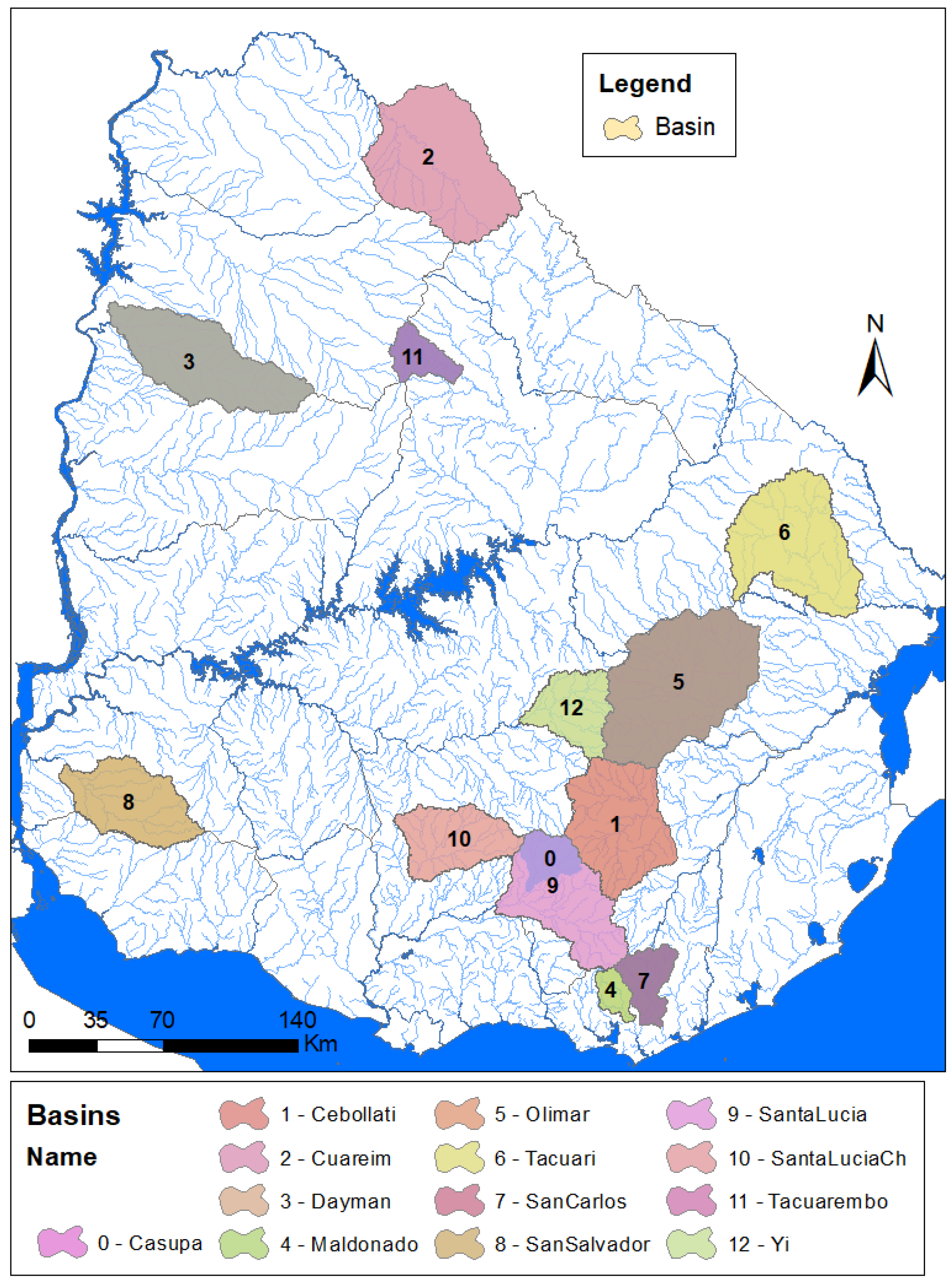
The study area covers 13 watersheds across Uruguay, having areas ranging from 300 to 5000 km² spread throughout northern and southern regions (Figure 1). These basins were selected based on three main criteria: (i) data quality; (ii) spatial distribution; (iii) rainfall-runoff model hypothesis (

Table 1. Criteria for watershed selection.

Criteria for Watershed Selections
Data Quality	Quality and availability of streamflow observations.
	Simultaneous precipitation and flow data.
Spatial Distribution	Watersheds distributed all over the country.
	Elevation covers the entire national range.
	Precipitation and temperature cover the entire national ranges.
	Different soil characteristics (dominant) considered.
Model Hypothesis	Adequate surface to the model-unit hydrograph.
	No presence of reservoirs.

). The annual mean precipitation is 1250–1450 mm in the northern region and 1050–1250 mm in the southern part. The average air temperature varies between 2 and 3 °C in northern and southern areas. In particular, in the northern regions, the average air temperature ranges approximately between 25 °C (in January) and 13 °C (in July); and in the southern areas, it ranges between 22 °C (in January) and 11 °C (in July). The relief varies between 0 m and 500 m above mean sea level (m.s.l.) in the entire country. Natural watersheds both in the southern and in the northern region are mostly covered with natural grassland (freely downloadable from the National Environmental Observatory of Uruguay (OAN) [35]).

In

Table 2. Catchment and hydrologic characteristics of the 13 selected watersheds.

Basin		Catchment Characteristics				Hydrologic Characteristics
ID	Name	Area (km2)	Slope (%)	Tc (h)	AD (mm)	R-B Index	Dominant Q (m3/s/km2)
0	Casupa	689	5.4	16	77	0.50	0.14
1	Cebollati	2884	6.2	38	76	0.43	0.34
2	Cuareim	4568	4.4	50	37	0.50	0.13
3	Dayman	3183	2.5	44	78	0.46	0.51
4	Maldonado	366	8.4	12	72	0.45	0.24
5	Olimar	4679	6.6	43	86	0.35	0.37
6	Tacuari	3544	5.1	54	107	0.32	0.49
7	San Carlos	803	8.3	18	74	0.61	0.28
8	San Salvador	2151	2.4	38	125	0.48	0.39
9	Santa Lucia	2754	6.0	36	81	0.50	0.27
10	Santa Lucía Ch.	1749	3.3	26	99	0.78	0.44
11	Tacuarembo Ch.	660	6.8	23	77	0.63	0.71
12	Yi	1380	4.2	26	76	0.50	0.21

, the catchment and hydrologic characteristics of the selected watersheds are reported. Among the catchment characteristics, basin area (km²), slope (%), concentration-time (Tc) (h), and available water content (AD) (mm) were considered. To represent the hydrologic signature of the watersheds, the Richards–Baker Flashiness Index (R-B index) and the dominant discharge (Dominant Q) were calculated.

The R-B index measures the absolute day-to-day fluctuations inflow relative to total discharge and provides a useful characterization of the streamflow variability. This index can be used to classify a stream as stable or flashy, and it is defined in Equation (1) [36].

$$R-B index = \frac{{{\displaystyle \sum }}_{i=1}^n\left|Q_i-Q_{i-1}\right|}{{{\displaystyle \sum }}_{i=1}^n{Q}_i}$$

(1)

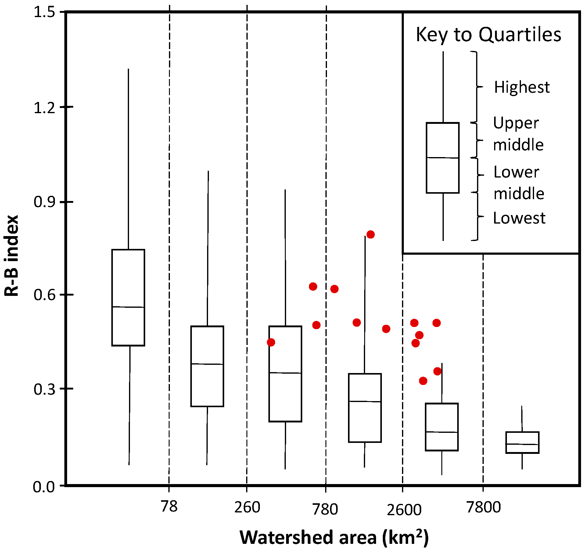
where Q_i is the mean daily flow on a given day i, and n is the number of days of recorded data at a given gauging station. To better classify streamflow, Baker et al. coupled R-B index with the surface watershed [36]. In particular, they represented 27-year average index values by box plots for six ranges of catchment size. The box plots divide the range of R-B values into quartiles, with the first quartile having the most stable streams and the fourth quartile having the flashiest (Figure 2). The watersheds selected for this work present an R-B index that ranges between 0.32 and 0.78 and their surface ranges between 366 km² and 4679 km². Based on the box plots shown in Figure 2, they are all located in the upper-middle/highest quartile, and therefore, they are classified as flashy.

The Dominant Q is a geomorphological concept and not strictly a measurable parameter. It represents a balance between the flows and sediments that shape the channel, the processes by which channel form is changed, and the ability of the boundary materials to resist change [37]. In this study, it was calculated by selecting a discharge based on a specified recurrence-interval discharge, typically between the 1 and 3-year events in the annual maximum series (2 years was chosen in this study). The annual series of maximum flow was adjusted to the generalized extreme value (GEV) distribution.

2.2. Data Collection

2.2.1. Precipitation, Climate, and Streamflow

Daily precipitation data (for the period 2001–2010) from 59 stations belonging to the National Institute of Meteorology (INUMET) and National Administration of Power Plants and Power Transmissions (UTE) was used in this study. The data quality was studied and analyzed, evaluating the accumulated annual rainfall (double mass curve) and the number of days with missing data. Furthermore, the records of 5 meteorological stations belonging to the National Institute of Agricultural Research (INIA) were taken into account. The latter, apart from the precipitation, provided climate data, including average air temperature (°C), average relative moisture (%), average wind speed (knots), and solar radiation (h). With this information, it was possible to calculate the potential evapotranspiration (PET) using the Penman-Monteith method.

Daily streamflow data (for the period 2001–2010) from 13 hydrometric stations belonging to the Uruguayan National Water Board (DINAGUA) was used. To ensure the quality of the data collected, a consistency analysis of the water balance was carried out, taking into account precipitation, evapotranspiration, streamflow, and the calculation of the runoff coefficient.

In Figure 3, the location of the selected pluviometric stations is shown with blue dots, the 5 meteorological stations are represented with pink squares, while the hydrometric stations are symbolized with red triangles.

2.2.2. Soil Type

The information about the soil types with a scale 1:40,000 was obtained from the General Directorate of Natural Resources of the Ministry of Livestock, Agriculture, and Fisheries (RENARE-MGAP). This map is known as CONEAT soil map, where CONEAT stands for the National Commission for the Agro-economic Study of the Earth (COmisión Nacional de Estudio Agro económico de la Tierra), that represents the name of the commission which developed the index CONEAT. This index characterizes the average productivity of the soils contained within one property. The Uruguayan soil has been categorized into 188 different types, each category with an associated productivity index. Among other information, this map provides the amount of available water content (AD) for each soil type. AD was calculated considering the thickness of soil horizons, the percentage of sand, silt, clay, and organic matter presented in each soil unit [38,39,40] (see Supplementary Materials (SM-1) for more information about the calculation of AD).

2.3. Rainfall-Runoff Model

The GR4J model (which stands for modèle du Génie Rural à 4 paramètres Journalier), a daily lumped four-parameter rainfall-runoff model, was used in this work. The GR4J model by Perrin et al. [41] is the modified version of the GR3J model initially proposed by Edijatno and Michel [42] and then successively improved by Nascimento and Edijatno et al. [43,44].

A well-known conceptualization of the model structure is shown in Figure 4, and the parameter description is reported in

Table 3. Description of the GR4J-model parameters.

Parameter	Description	Unit
x1	Maximum capacity of the production store	mm
x2	Groundwater exchange coefficient	mm
x3	Capacity of the nonlinear routing store	mm
x4	Unit-hydrograph time base	day

.

The model belongs to the family of conceptual lumped models. It is characterized by two reservoirs or stores: a production store, which computes effective rainfall, and a routing store combined with a unit hydrograph for water transfer. The input model data are precipitation (P) and potential evapotranspiration (PE), and they are used to calculate streamflow. This calculation is made in three steps: first, the effective rainfall is calculated with a zero capacity interception store and a soil moisture accounting store. Second, this effective rainfall is split into two components: one routes 90% of effective rainfall with a unit hydrograph UH1 and a nonlinear routing store; the other routes the remaining 10% with a second unit hydrograph UH2. Third, an inter-catchment groundwater flow function is computed to account for water gains or losses stemming from interactions with neighboring catchments or groundwater and is added to both components. The final discharge at the catchment outlet is calculated as the sum of both flow components.

The GR4J model parameters were calibrated on donor catchments and subsequently transferred to acceptors catchments. To test the performance of the rainfall-runoff model, the coefficient of determination (R²) (Equation (2)), Nash–Sutcliffe efficiency (NSE) (Equation (3)), and index of agreement (d) (Equation (4)) were used as metrics:

$$R^2={\left\{\frac{1}{N}\frac{{{\displaystyle \sum }}_{t=1}^N\left[\left(x_{obs}\left(t\right) - {\mu }_{obs}\right)\left(x_{sim}\left(t\right) - {\mu }_{sim}\right)\right]}{{\sigma }_{obs}{\sigma }_{sim}}\right\}}^2$$

(2)

$$\mathrm{NSE}=1 - \frac{{{\displaystyle \sum }}_{t=1}^N{\left[x_{obs}\left(t\right)-x_{sim}\left(t\right)\right]}^2}{{{\displaystyle \sum }}_{t=1}^N{\left[x_{obs}\left(t\right) - {\mu }_{obs}\right]}^2}$$

(3)

$$d=1 - \frac{{{\displaystyle \sum }}_{i=1}^N{\left[x_{obs}\left(t\right) - x_{sim}\left(t\right)\right]}^2}{{{\displaystyle \sum }}_{i=1}^N{\left[\left|x_{sim}\left(t\right) - {\mu }_{obs}\right| - \left|x_{obs}\left(t\right) - {\mu }_{obs}\right|\right]}^2}$$

(4)

where x_obs(t) is the observed value at the time step t, x_sim(t) is the simulated value, being (μ_sim, σ_sim) and (μ_obs, σ_obs) the first two statistical moments (means and standard deviations) of x_sim and x_obs, respectively, over the entire simulation period of length N.

2.4. Cluster Analysis for Watershed Selection

Conventional multivariate data-analysis techniques, principal component analysis (PCA) and cluster analysis (CA) (k-means), were used in this study to assure that watersheds with different hydrologic signature, and therefore with different physical and climate characteristics, were considered. Furthermore, the clustering method helps in reducing the computation time of the cross-validation.

The goal of the clustering algorithm is to partition a complex dataset into homogeneous clusters, such that the between-group similarities are smaller than the within-group similarities [45,46]. These clusters can reveal patterns related to the phenomenon under study. A distance function measures the similarity between observations. Firstly, the similarity is calculated between the data points. Once the data points begin to be grouped into clusters, the similarity is computed between the groups as well. Several metrics could be used to calculate it, and the choice of the similarity measure could influence the results [47]. This technique also requires a prior choice of the number of groups (k) that is arbitrary. In this study, the silhouette method was used to calculate the optimal k [48]. This analysis measures how close each point in a cluster is to the points in its neighboring clusters:

$$s\left(i\right)=\frac{b\left(i\right) - a\left(i\right)}{\max \left(b\left(i\right),a\left(i\right)\right)}$$

(5)

where a(i) is the average distance of the point (i) to all the other points in the cluster it is assigned (A), b(i) is the average distance of the point (i) to other points to its closest neighboring cluster (B).

Silhouette values lie in the range of [−1, 1]; the higher the value, the better is the cluster configuration. In particular, the value 1 is ideal since it indicates that the sample is far away from its neighboring cluster and very close to the group it is assigned. Similarly, the value −1 is the least preferred since it indicates that the point is closer to its neighboring cluster than to the cluster it is assigned.

2.5. Regionalization Approach

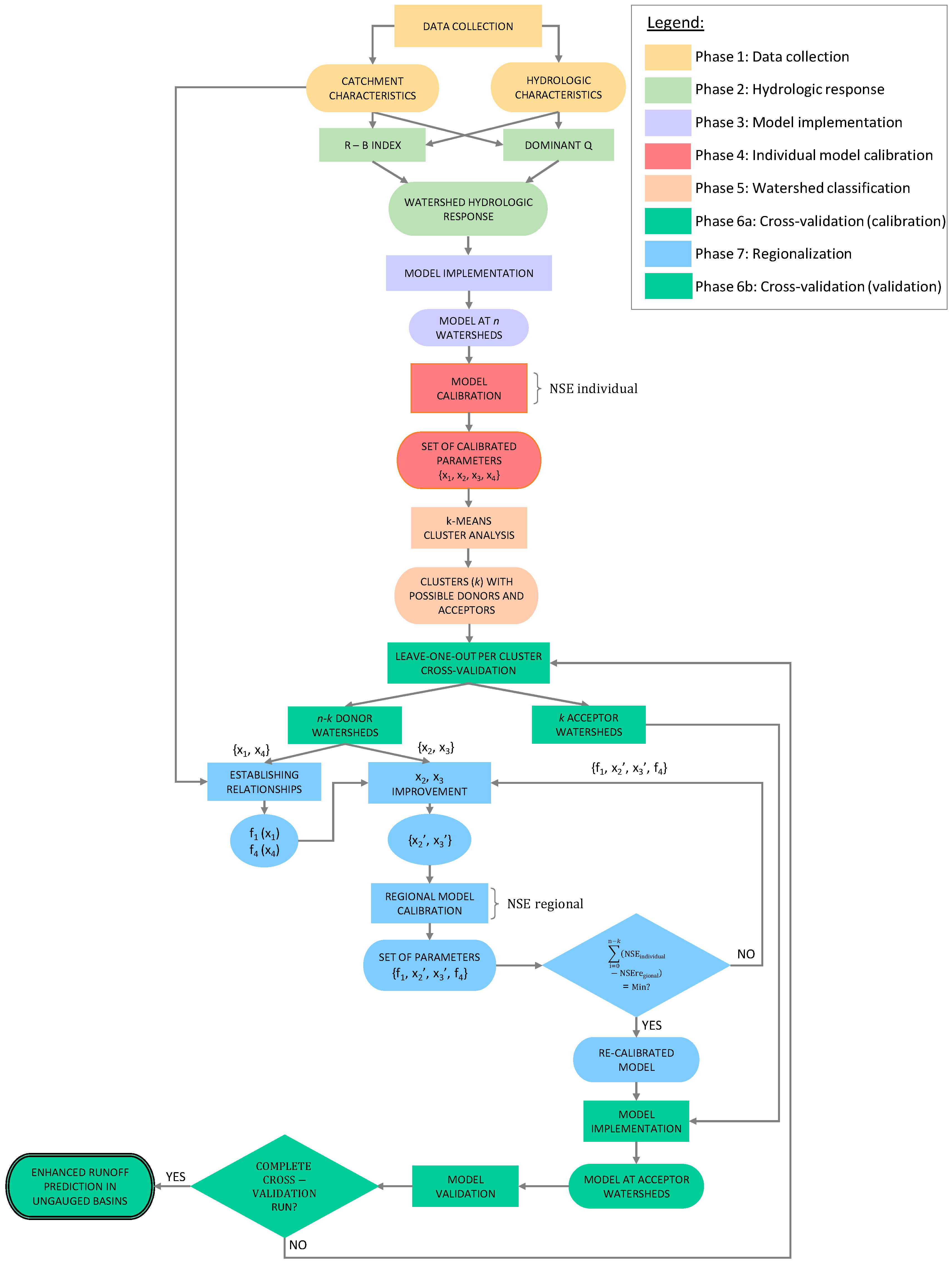
The new study approach is summarized in 7 phases as follows (Figure 5).

Phase 1: Data collection. The required input data were adequately collected: (i) physical catchment characteristics, e.g., DEM and soil type; and (ii) climatic/hydrologic characteristics, e.g., flow, precipitation, and climate.

Phase 2: Hydrologic response. The runoff signature of the studied watersheds was evaluated by calculating the R-B index and dominant discharge.

Phase 3: Model implementation. The rainfall-runoff model was implemented at the n catchments by exploiting the input data collected during Phase 1.

Phase 4: Individual model calibration. Model parameters were calibrated at each watershed. Model performance was assessed by comparing the predicted and observed runoff at donor catchments. With this aim, Nash-Sutcliffe efficiency (NSE_individual) was used as an objective function, coefficient of determination (R²) and index of agreement (d) as performance indicators.

Phase 5: Watershed classification. To assure the heterogeneity of the watersheds considered in terms of hydrologic signature, the catchments were clustered into k different groups according to their hydrologic and physical similarity (calculated in Phase 2). This phase will also reduce the computation time of the cross-validation phase.

Phase 6a: Leave-one-out cross-validation (calibration). The watersheds were divided into n-k donors and k acceptors.

Phase 7: Enhanced regionalization (Regional model calibration). This step is performed inside the cross-validation phase. Functional relationships between model parameters and physical-catchment attributes were established (f₁(x₁), f₄(x₄)). By considering f₁ and f₄ instead of x₁ and x₄, a regional model calibration was carried out (NSE_regional was used as a performance indicator) to find the pair {x₂, x₃} that minimize ${\displaystyle \sum }_{i=1}^{n-k}\left(NS{E}_{individual}-NS{E}_{regional}\right)$, where n-k represents the number of donor catchments.

Phase 6b: Leave-one-out cross-validation (validation). The performance of the proposed regionalization approach was evaluated (NSE_regional). The runoff output of the model with the regionalized and optimal calibrated parameters at each acceptor watershed was implemented at the k donors.

For the sake of clarity, it is worth mentioning that, in Figure 5, the input/output is represented with a circle, the output of the whole approach with a double-circle, and the processes with a rectangle.

3. Results and Discussion

3.1. Rainfall-Runoff Model Performance

The four parameters described in Table 3 were used to calibrate the rainfall-runoff model at each watershed. The 80% confidence intervals for the four parameters and the values chosen for each of them at each basin are shown in

Table 4. Approximate 80% confidence intervals for the four parameters (Adapted from [41]).

Parameter	80% Confidence Interval
x1 (mm)	[100, 1200]
x2 (mm)	[−5, 3]
x3 (mm)	[20, 300]
x4 (day)	[1.1, 2.9]

and

Table 5. Parameters of the rainfall-runoff model for the individual calibration.

Basin	x1	x2	x3	x4
Casupa	91	−2.5	70.0	2.0
Cebollati	90	0.5	70	2.7
Cuareim	105	1	25	2.4
Dayman	91	0.5	80.0	2.4
Maldonado	70	1	34	2.2
Olimar	105	0.5	80	3
San Carlos	100	0	30	2.3
San Salvador	130	1	15	2.6
Santa Lucia	100	−1	30	2.5
Santa Lucía Ch.	101	−2.5	49	2.3
Tacuarembo Ch	60	2	34.0	2.5
Tacuari	130	−2	110	3.3
Yi	100	−2.5	80	2.5

, respectively.

The values of x₁ are lower than the median value of its range (median = 350). Four of the values are even lower than the minimum presented in Table 4. This is justified by the fact that the Uruguayan soils are not thick and are characterized by expanded clay formed by minerals that, with water, increase their volume and reduce soil-storage capacity [49]. Therefore, Uruguayan soils are characterized by a very low soil-water availability. The values of x₄ are in the upper border of its range. Two of the values are higher than the maximum presented in Table 4. This depends on the watershed surface: the higher the area, the higher the influence of small flood-plain storages within the basin, the higher x₄.

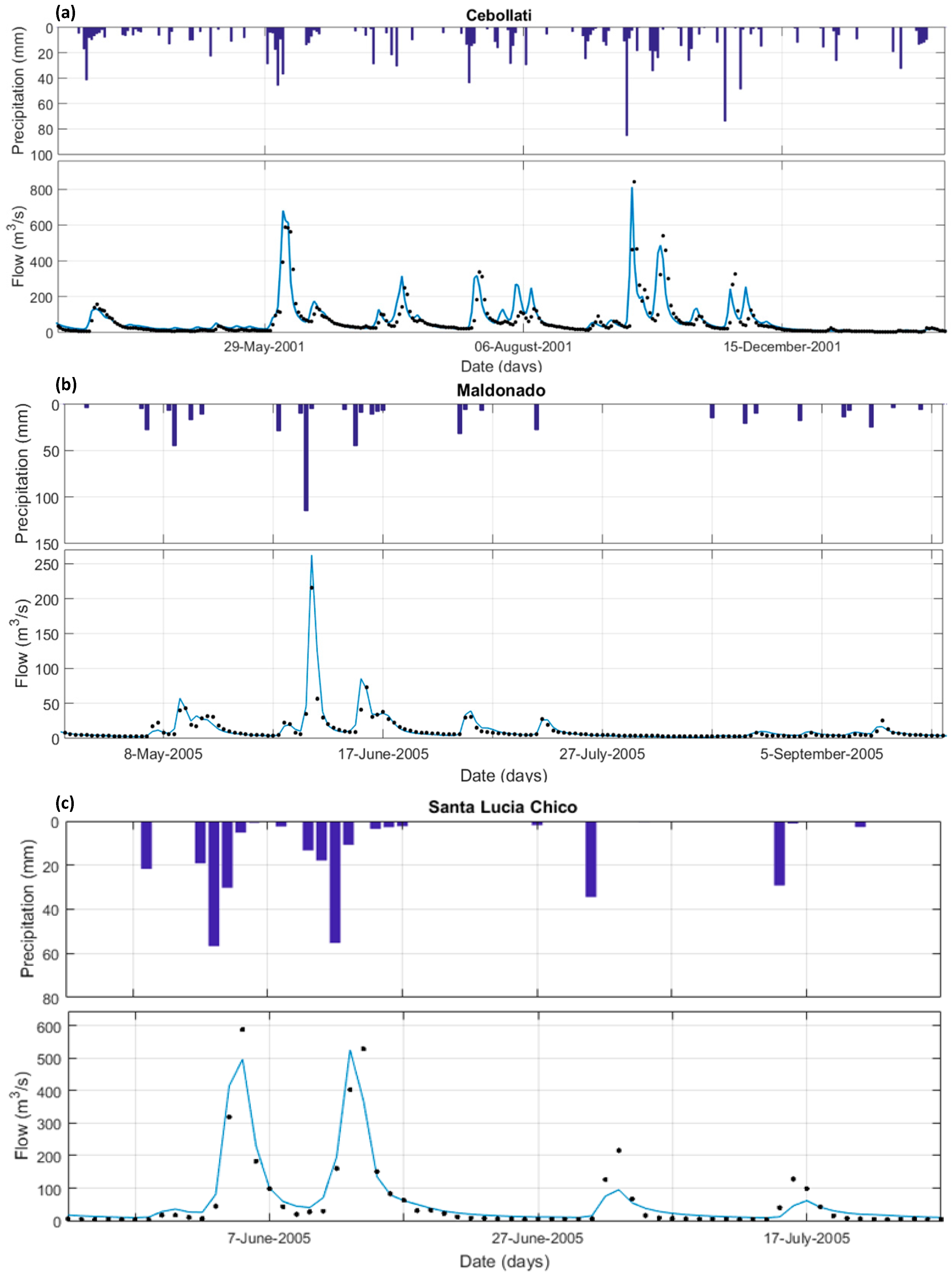
The calibration of the rainfall-runoff model employed an iterative process by varying the parameters in Table 4. Working taking into account the established range, and comparing (graphically in Figure 6 and numerically in

Table 6. Numerical comparison between the simulated and measured hydrographs (individual model calibration).

Basin	NSE	R2	d
Casupa	0.84	0.68	0.74
Cebollati	0.83	0.91	0.84
Cuareim	0.81	0.90	0.74
Dayman	0.82	0.66	0.77
Maldonado	0.80	0.90	0.81
Olimar	0.77	0.92	0.77
San Carlos	0.85	0.92	0.84
San Salvador	0.70	0.84	0.79
Santa Lucía	0.84	0.93	0.86
Santa Lucía Chico	0.68	0.83	0.76
Tacuarembó Chico	0.94	0.75	0.81
Tacuari	0.74	0.86	0.77
Yi	0.73	0.86	0.80

) the simulation with the measured hydrograph, the calibration was individually performed for each watershed until a good fit was obtained (individual model calibration). In particular, NSE was used as an objective function, and R² and d were used to evaluate the model performance. The period of calibration ranged between 2 and 5 years, depending on the data availability and data quality at each basin. In Figure 6, we are showing the comparison between measured and simulated streamflow of three basins significantly different among each other (Cebollati, Maldonado, and Santa Lucía Chico) for different time windows.

The agreement between measured and simulated hydrographs for all simulations was very satisfactory. In Figure 7, the statistical results of the individual calibration process at each selected watershed are represented. They follow the general performance ratings for adopted statistics by Moriasi et al. [50] and Chen et al. [51] reported in

Table 7. General performance ratings for adopted statistics.

Performance Rating	R2	NSE	d
Very good	0.75 < R2 ≤ 1.00	0.75 < NSE ≤ 1.00	0.75 < d ≤ 1.00
Good	0.65 < R2 ≤ 0.75	0.65 < NSE ≤ 0.75	0.65 < d ≤ 0.75
Satisfactory	0.50 < R2 ≤ 0.65	0.50 < NSE ≤ 0.65	0.50 < d ≤ 0.65
Unsatisfactory	R2 ≤ 0.50	NSE ≤ 0.50	d ≤ 0.50

.

3.2. Donor and Acceptor Catchment Selection

To assure the validity of the new regionalization approach to catchments characterized by different weather conditions, prior to implementing the cross-validation and regionalization approach, the 13 watersheds have been classified on the basis of their physical and hydrologic characteristics. With this aim, principal component analysis (PCA) associated with k-means clustering was applied to watershed attributes to classify the basins into k clusters.

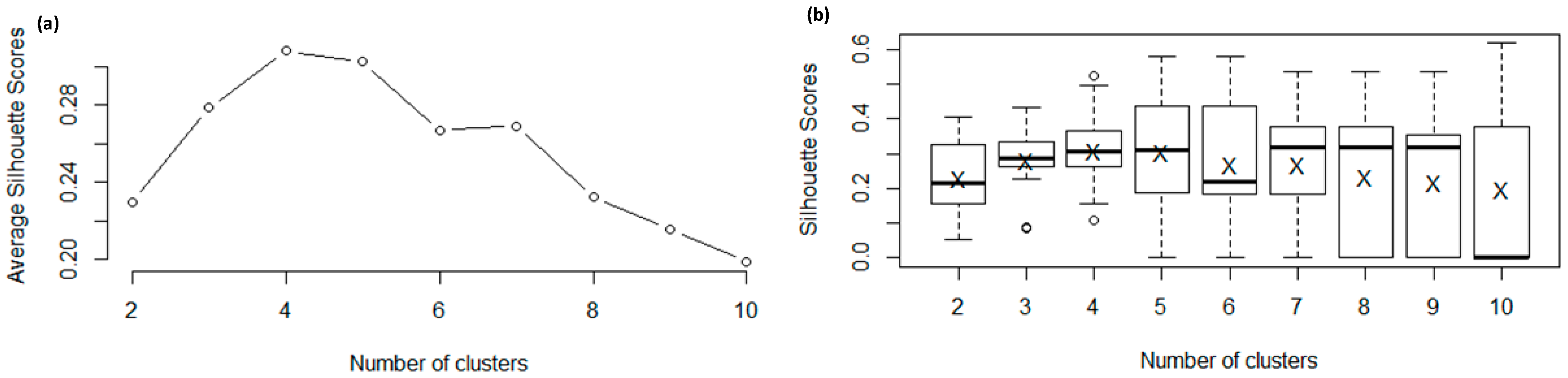
The silhouette method was adopted to identify the optimum number of clusters (k) to consider. The average silhouette score of all the examples in the data set was calculated (Figure 8a). This gives us one value representing the silhouette score of the entire cluster. Furthermore, the silhouette-score boxplot was represented to evaluate the dispersion of the data at each number of clusters considered. (Figure 8b). Since there were 13 watersheds, the possibility of having k = 2 to k = 10 was taken into account.

From Figure 8a, it seems that the optimum number of clusters is k = 4. However, in Figure 8b, it is possible to see that the dispersion of the data related to k = 4 is higher than k = 3. Furthermore, the k = 3-average is only slightly lower than the average on k = 4, and its minimum is higher than k = 4. For these reasons, we decided to group the watersheds into 3 clusters.

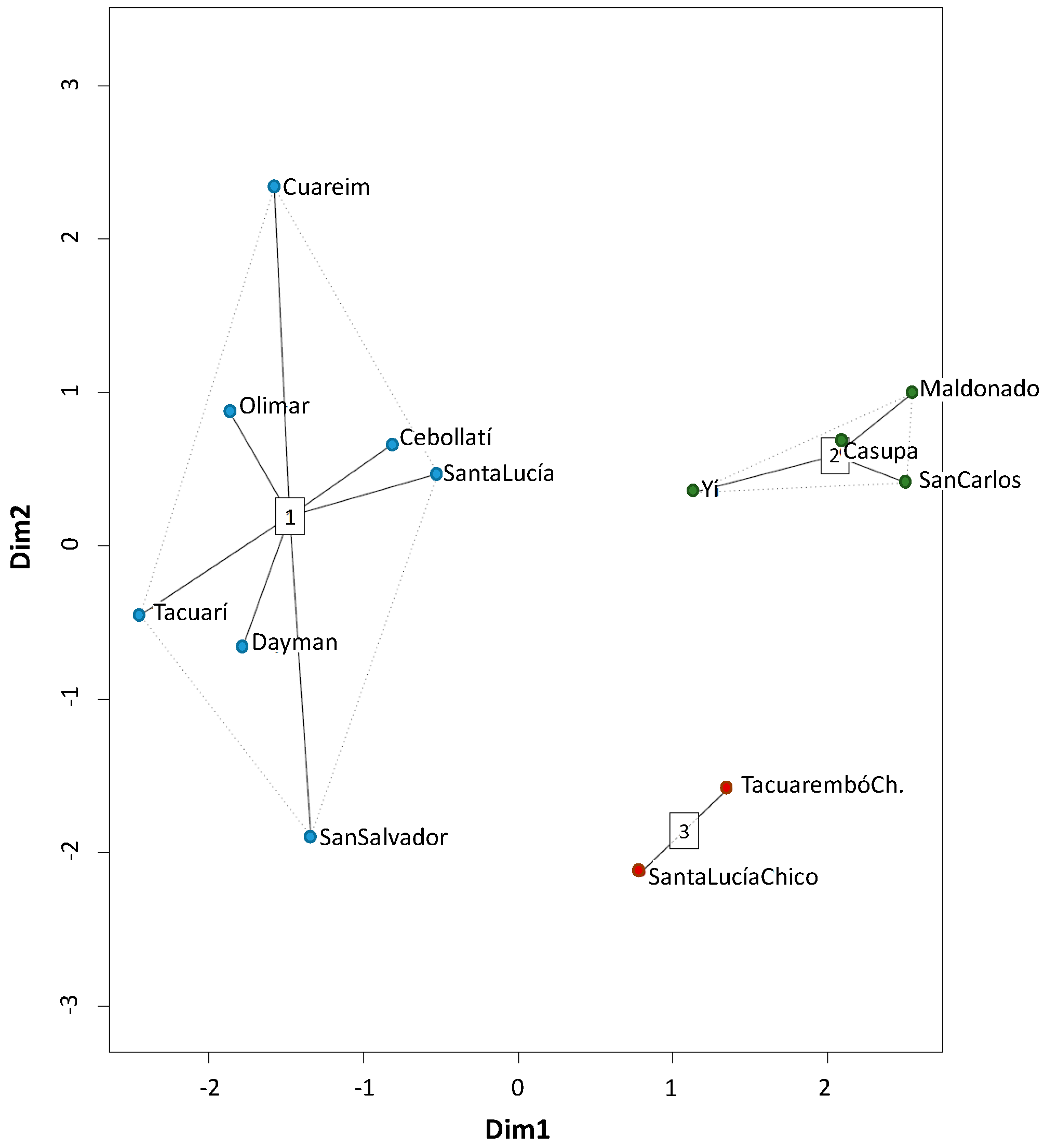
The PCA/k-means analysis was coded and run in R [52], by using the libraries “cluster,” “HSAUR,” and “vegan.” The attributes considered were watershed area (km²), slope (%), concentration-time (h), and AD (mm), for considering the physical catchment characteristics; R-B index, and Dominant Q (m³/s/km²), for taking into account the hydrologic response. A data matrix (13 × 7) was the input for this HCA, being 13 watersheds and 7 attributes (6 basin characteristics + 1 basin identification). Prior to classification, the attributes (raw data) were mean-centered and scaled to unit variance to give equal importance to each attribute and to handle the different measurement units of attributes. After the normalization, all attributes had mean equal to zero and standard deviation equal to one. The first two principal components (PCs) or dimensions (Dim) were selected since they represented 72% of the variance. In Figure 9, the resulting PCA scores plot is shown. Each of the 13 watersheds is represented by a data point in the plot, and their location indicates the score of each basin for the PCs.

3.3. Calibration and Model Parameter Regionalization

To evaluate the runoff predictions in ungauged watersheds, three of the thirteen catchments, each of them belonging to the three clusters k, were left out in turn and considered as ungauged or acceptor watersheds. Therefore, the performance of this methodology is successfully validated (with leave-one-out cross-validation) by assuming each gauged catchment, belonging to each cluster, as ungauged at once. From the donor catchments, the entire set of regionalized and optimal calibrated parameters is then used to model runoff at the “ungauged” catchments. This is then compared with the streamflow measurements to finalize the validation of the proposed approach.

The regionalization phase is located inside the cross-validation process; particularly between the calibration and validation stage (Figure 1).

A relationship between model parameters and physical basin characteristics was found. In particular, a relationship of this kind was established for x₁ and x₄.

x₁ was directly associated with the average of AD in the soil, which represents the maximum amount of water useful for the vegetation for the evapotranspiration process. It is calculated by subtracting field capacity and wilting point.

$$x_1 = AD$$

(6)

x₄ was found to be correlated with the concentration-time (Tc) of the basins. The best approximation to the Tc and x₄ was obtained using a relationship described by a power law. These curves are graphically reported in the Supplementary Materials (SM-2), and the following one has been considered as an average curve that represents all of them:

$$x_4=1.24·T_c{}^{0.205}$$

(7)

The agreement among x₄ − Tc data points and the regression (Equation (7)) was evaluated through the R², which was equal to 0.55.

Since no relationships between x₂ and x₃ with physical catchment characteristics were found, we proceeded with a regional model calibration to compute the optimal values for these two parameters. For doing this, a unique set of parameters for the 10 watersheds has to be found (where 10 is obtained from n − k = 10 − 3). Therefore, x₁ and x₄ were fixed on the basis of the correlations previously mentioned, and an iterative process was employed by varying x₂ and x₃ working within the established ranges. The regional calibration was performed until a good fit was obtained, i.e., when the difference between the NSE obtained from the individual calibration (NSE_individual), and the NSE obtained from the current calibration (NSE_regional) was minimum (Equation (8)). Among the three selected goodness-of-fit indicators (Equations (2)–(4)), NSE was chosen since it is the most restrictive one.

$${\displaystyle \sum }_{i=1}^{10}(NSE {individual}_i-NSE {regional}_i)$$

(8)

In this calibration process, the 10 donor watersheds were considered. It is worth remarking that these 10 watersheds are different at any iteration of the cross-validation process. In particular, considering that three clusters were identified and each of them contains seven, two, and four elements respectively (Figure 9), 56 iterations were computed for the cross-validation process. As partial outcomes, in

Table 8. Partial result: range of variation of NSE in the first stage of the cross-validation process (calibration).

Basin	NSE Max	NSE Min
Casupa	0.72	0.64
Cebollati	0.82	0.80
Cuareim	0.65	0.49
Dayman	0.73	0.70
Maldonado	0.77	0.72
Olimar	0.76	0.74
San Carlos	0.81	0.75
San Salvador	0.57	0.50
Santa Lucía	0.78	0.75
Santa Lucía Chico	0.52	0.48
Tacuarembó Chico	0.82	0.79
Tacuari	0.70	0.63
Yi	0.69	0.62

, the range of variation of NSE for the calibration process is presented.

It is worth noting that NSE is never lower than 0.5. Therefore, all the iterations can be considered satisfactory, good, and very good, based on the classification reported in Table 7.

3.4. Cross-Validation of the Regionalization Process

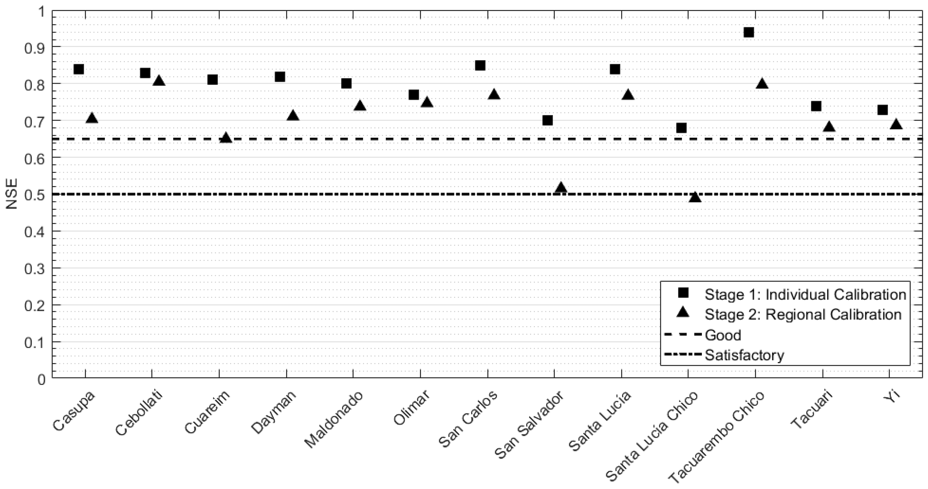
The improved regionalization method was tested at the acceptor basins. The streamflow prediction was then compared to the observed streamflow time-series at the pseudo-ungauged catchments. In Figure 10, the performance obtained at the individual calibration phase and regional calibration stage were evaluated by NSE. The numerical values for this final stage (regional model calibration) are reported in

Table 9. Numerical comparison between the simulated and measured hydrographs at acceptor catchments (validation of the enhanced regionalization process).

Basin	NSE	R2	d
Casupa	0.70	0.84	0.74
Cebollati	0.81	0.90	0.82
Cuareim	0.65	0.68	0.76
Dayman	0.71	0.82	0.78
Maldonado	0.74	0.87	0.77
Olimar	0.75	0.90	0.82
San Carlos	0.77	0.88	0.81
San Salvador	0.52	0.73	0.78
Santa Lucía	0.77	0.87	0.82
Santa Lucía Chico	0.49	0.67	0.78
Tacuarembo Ch.	0.80	0.94	0.82
Tacuari	0.68	0.80	0.79
Yi	0.69	0.87	0.80

. Considering that in the 56 iterations, x₂ and x₃ were varying in the ranges [−1.5, −0.5] and [47, 67] respectively, it is worth remarking that the following outcomes correspond to the best values of x₂ = −1.5 and x₃ = 59.

The GR4J model has obtained very good regionalized results by using the hydrologic and physical similarity approach. The NSE values vary from 0.49 (Santa Lucía Chico basin) to 0.81 (Cebollati basin), with an average equal to 0.70; the R² values vary from 0.67 (Santa Lucía Chico basin) to 0.94 (Tacuarembo Ch. basin), with an average equal to 0.83; the d values vary from 0.74 (Casupa basin) to 0.82 (Cebollati, Olimar, Santa Lucía, and Tacuarembo Ch. basins), with an average equal to 0.79. Overall, the agreement between measured and simulated hydrographs for all simulations was very satisfactory. From Figure 10, poorer performance was found only for San Salvador and Santa Lucía Chico watersheds for the regional calibration (NSE = 0.52 and NSE = 0.49, respectively). This can be caused by different reasons. (i) Santa Lucía Chico watershed lacks a good spatial distribution of pluviometric stations: two rain gauges located on the eastern border, two rain gauges in the north and one in the south (not belonging to the basin) were used to represent the precipitation distribution of this catchment (Figure 4). (ii) Another significant reason is represented by the low data quality in San Salvador watershed. (iii) It is essential to remark that San Salvador and Santa Lucía Chico are among the basins characterized by the lowest slope and the highest AD. Knowing that the GR4J model better simulates watersheds with a rapid hydrologic response [53,54,55], it is clear that this model is not the most suitable one for San Salvador and Santa Lucía Chico basins. This is confirmed by the fact that NSE values obtained from the individual calibration (Stage 1) were already the lowest among the 13.

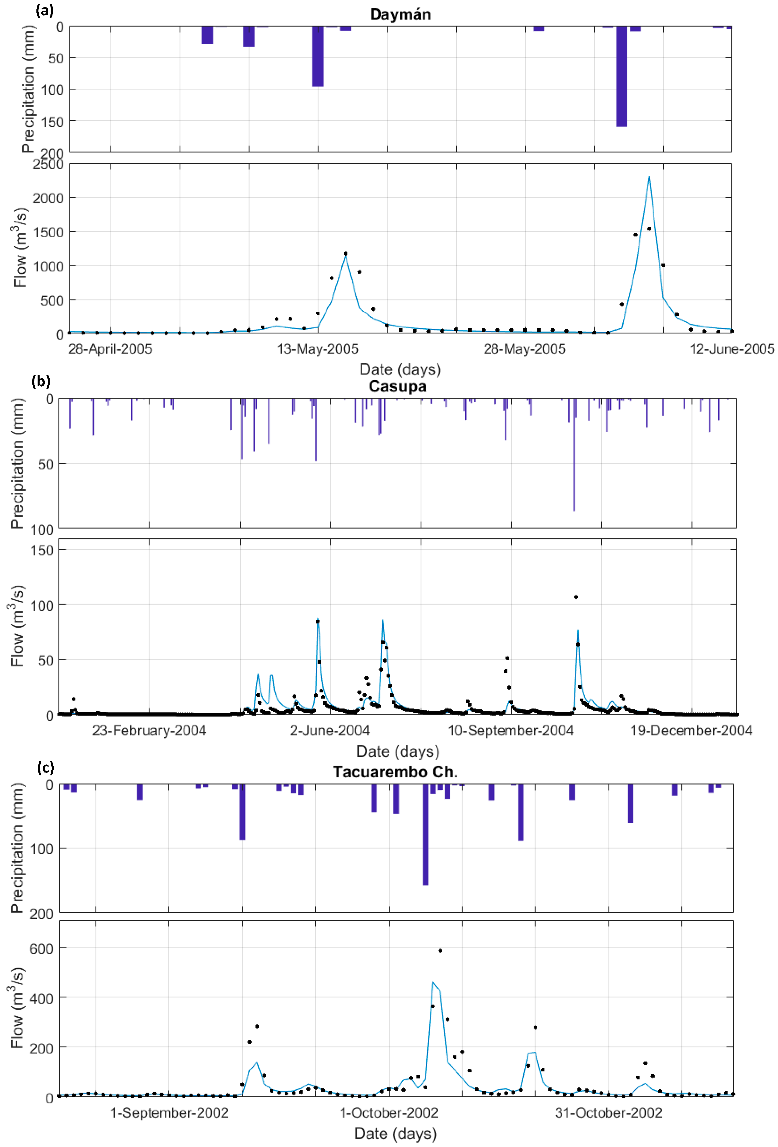
In Figure 11, the graphical comparison between observed and simulated hydrographs at three acceptor watersheds is shown. For this representation, the closest basins to the centroid of each cluster were considered. For the sake of completeness, the range of variation of NSE in the last stage of the cross-validation process (validation), and the graphical comparison between observed and simulated flow-duration curve (FDC) are reported in the Supplementary Materials (SM-3 and SM-4 respectively).

It is important to examine if the performance of the regionalization process changes with an individual attribute in catchments. A correlation matrix was analyzed, considering the regionalized values of the goodness-of-fit indicators and the physical and hydrologic catchment characteristics (

Table 10. Correlation matrix of basin characteristics and regionalized goodness-of-fit indicators.

	R2	NSE	d	Area	Slope	Tc	AD	R-B index	Dominant Q
R2	1.0
NSE	0.9	1.0
d	0.8	0.7	1.0
Area	−0.3	0.0	0.2	1.0
Slope	0.7	0.7	0.4	−0.3	1.0
Tc	−0.3	−0.1	0.2	0.9	−0.5	1.0
AD	−0.1	−0.5	0.0	−0.1	−0.3	0.1	1.0
R-B index	−0.3	−0.4	−0.4	−0.5	−0.1	−0.5	−0.1	1.0
Dominant Q	0.2	0.0	0.3	0.0	−0.1	0.2	0.5	0.2	1.0

).

There exists a strong direct relationship between the regionalized R², NSE, and catchment slope. The regionalized model performance tends to increase with an increase in slope. However, a decreasing trend is shown between AD and the regionalized NSE. This suggests that regionalization results tend to become better in steep-slope watersheds characterized by a low amount of available water content in their soils; e.g., watersheds with a high-runoff potentiality (flashy). The latter is justified from the fact that if Slope decreases and/or AD increases, considering a hypothetical output hydrograph, the superficial runoff contribution is reduced in favor of the contribution given by the groundwater flow (base flow + slow sub-surface flow). This reality cannot be well depicted in the GR4J model since it better simulates watersheds with a rapid hydrologic response. This result is generally in accordance with the regionalization results found in other regions, such as Australia, Asia, and Europe [53,54,55].

4. Summary and Conclusions

In this study, we proposed an improved regionalization approach that is valid at country scale and for those regions characterized by highly variable-climatic conditions. It was successfully applied to several gauged and pseudo-ungauged basins in Uruguay, a country whose climate is influenced by the ENSO.

A daily rainfall-runoff model, GR4J, was implemented and successfully calibrated at 13 watersheds (individual calibration) (NSE_average = 0.80; R²_average = 0.84; d_average = 0.79). To assure the validity of the new regionalization approach to catchments characterized by different weather conditions, prior to implementing the regionalization approach and the cross-validation process, the 13 watersheds were classified on the basis of their physical and hydrologic characteristics with the aid of PCA/k-means techniques.

After finding the optimal set of parameters of the hydrologic model at each basin, the proposed approach does not just transfer it to a similar ungauged watershed, but it finds robust relationships between x₁ and AD (called f₁) and between x₄ and T_c (called f₄). These correlations were then exploited for a regional model calibration that allowed to generate a calibrated set of parameters that was transferred to the basin acceptors for cross-validating the model and testing the accuracy and reliability of this new regionalization approach. Model performance was very satisfactory (NSE_average = 0.70; R²_average = 0.83; d_average = 0.79). It was found that the regionalized R² and NSE are directly correlated with catchment slope and inversely correlated with AD and surface basin, among the other variables. This suggests that regionalization results tend to become better in medium/small and steep-slope watersheds characterized by a low amount of available water content in their soils, e.g., watersheds with a high-runoff potentiality.

This paper not only provides an enhanced regionalization approach to predict runoff time series in ungauged catchments at country scale under highly variable-weather conditions, but also provides guidelines for a proper implementation of the GR4J model.

References

- Yang, X.; Magnusson, J.; Xu, C.-Y. Transferability of regionalization methods under changing climate. J. Hydrol. 2019, 568, 67–81. [Google Scholar] [CrossRef]
- Gorgoglione, A.; Gioia, A.; Iacobellis, V. A Framework for Assessing Modeling Performance and Effects of Rainfall-Catchment-Drainage Characteristics on Nutrient Urban Runoff in Poorly Gauged Watersheds. Sustainability 2019, 11, 4933. [Google Scholar] [CrossRef] [Green Version]
- Gorgoglione, A.; Bombardelli, F.A.; Pitton, B.J.L.; Oki, L.R.; Haver, D.L.; Young, T.M. Uncertainty in the parameterization of sediment build-up and wash-off processes in the simulation of water quality in urban areas. Environ. Model. Softw. 2019, 111, 170–181. [Google Scholar] [CrossRef]
- Sivapalan, M.; Takeuchi, K.; Franks, S.W.; Gupta, V.K.; Karambiri, H.; Lakshmi, V.; Liang, X.; McDonnell, J.J.; Mendiondo, E.M.; O’Connell, P.E.; et al. IAHS Decade on Predictions in Ungauged Basins (PUB), 2003–2012: Shaping an exciting future for the hydrological sciences. Hydrol. Sci. J. 2003, 48, 857–880. [Google Scholar] [CrossRef] [Green Version]
- Tsegaw, A.T.; Alfredsen, K.; Skaugen, T.; Muthanna, T.M. Predicting hourly flows at ungauged small rural catchments using a parsimonious hydrological model. J. Hydrol. 2019, 573, 855–871. [Google Scholar] [CrossRef]
- Nearing, G.S.; Ruddell, B.L.; Bennett, A.R.; Prieto, C.; Gupta, H. Does Information Theory Provide a New Paradigm for Earth Science? Hypothesis Testing. Water Resour. Res. 2020, 56, e2019WR024918. [Google Scholar] [CrossRef]
- Hrachowitz, M.; Savenije, H.H.G.; Blöschl, G.; McDonnell, J.J.; Sivapalan, M.; Pomeroy, J.W.; Arheimer, B.; Blume, T.; Clark, M.P.; Ehret, U.; et al. A decade of Predictions in Ungauged Basins (PUB)—A review. Hydrol. Sci. J. 2013, 58, 1198–1255. [Google Scholar] [CrossRef]
- Parajka, J.; Merz, R.; Blöschl, G. A comparison of regionalization methods for catchment model parameters. Hydrol. Earth Syst. Sci. Discuss. 2005, 2, 509–542. [Google Scholar] [CrossRef] [Green Version]
- Oudin, L.; Andréassian, V.; Perrin, C.; Michel, C.; Le Moine, N. Spatial proximity, physical similarity, regression and ungaged catchments: A comparison of regionalization approaches based on 913 French catchments. Water Resour. Res. 2008, 44, 1–15. [Google Scholar] [CrossRef]
- Reichl, J.P.C.; Western, A.W.; McIntyre, N.R.; Chiew, F.H.S. Optimization of a similarity measure for estimating ungauged streamflow. Water Resour. Res. 2009, 45, 1–15. [Google Scholar] [CrossRef] [Green Version]
- He, Y.; Bárdossy, A.; Zehe, E. A review of regionalization for continuous streamflow simulation. Hydrol. Earth Syst. Sci. 2011, 15, 3539–3553. [Google Scholar] [CrossRef] [Green Version]
- Samuel, J.; Coulibaly, P.; Metcalfe, R.A. Estimation of continuous streamflow in Ontario ungauged basins: Comparison of regionalization methods. J. Hydrol. Eng. 2011, 16, 447–459. [Google Scholar] [CrossRef]
- Razavi, T.; Coulibaly, P. Streamflow prediction in ungauged basins: Review of regionalization methods. J. Hydrol. Eng. 2013, 18, 958–975. [Google Scholar] [CrossRef]
- Salinas, J.L.; Laaha, G.; Rogger, M.; Parajka, J.; Viglione, A.; Sivapalan, M.; Blöschl, G. Comparative assessment of predictions in ungauged basins-Part 2: Flood and low flow studies. Hydrol. Earth Syst. Sci. 2013, 17, 2637–2652. [Google Scholar] [CrossRef] [Green Version]
- Viglione, A.; Parajka, J.; Rogger, M.; Salinas, J.L.; Laaha, G.; Sivapalan, M.; Blöschl, G. Comparative assessment of predictions in ungauged basins-Part 3: Runoff signatures in Austria. Hydrol. Earth Syst. Sci. 2013, 17, 2263–2279. [Google Scholar] [CrossRef] [Green Version]
- Bastola, S.; Ishidaira, H.; Takeuchi, K. Regionalisation of hydrological model parameters under parameter uncertainty: A case study involving TOPMODEL and basins across the globe. J. Hydrol. 2008, 357, 188–206. [Google Scholar] [CrossRef]
- Götzinger, J.; Bárdossy, A. Comparison of four regionalisation methods for a distributed hydrological model. J. Hydrol. 2007, 333, 374–384. [Google Scholar] [CrossRef]
- Bao, Z.; Zhang, J.; Liu, J.; Fu, G.; Wang, G.; He, R.; Yan, X.; Jin, J.; Liu, H. Comparison of regionalization approaches based on regression and similarity for predictions in ungauged catchments under multiple hydro-climatic conditions. J. Hydrol. 2012, 466, 37–46. [Google Scholar] [CrossRef]
- Zhang, Y.; Vaze, J.; Chiew, F.H.; Teng, J.; Li, M. Predicting hydrological signatures in ungauged catchments using spatial interpolation, index model, and rainfall–runoff modelling. J. Hydrol. 2014, 517, 936–948. [Google Scholar] [CrossRef]
- Swain, J.B.; Patra, K.C. Streamflow estimation in ungauged catchments using regionalization techniques. J. Hydrol. 2017, 554, 420–433. [Google Scholar] [CrossRef]
- Yang, X.; Magnusson, J.; Rizzi, J.; Xu, C.-Y. Runoff prediction in ungauged catchments in Norway: Comparison of regionalization approaches. Hydrol. Res. 2018, 49, 487–505. [Google Scholar] [CrossRef]
- Kay, A.L.; Jones, D.A.; Crooks, S.M.; Calver, A.; Reynard, S.N. A comparison of three approaches to spatial generalization of rainfall-runoff models. Hydrol. Process. 2006, 20, 3953–3973. [Google Scholar] [CrossRef]
- Samaniego, L.; Bárdossy, A.; Kumar, R. Streamflow prediction in ungauged catchments using copula-based dissimilarity measures. Water Resour. Res. 2010, 46, W02506. [Google Scholar] [CrossRef]
- Ayzel, G.V. Runoff predictions in ungauged Arctic basins using conceptual models forced by reanalysis data. Water Resour. 2018, 45, S1–S7. [Google Scholar] [CrossRef]
- Prieto, C.; Le Vine, N.; Kavetski, D.; García, E.; Medina, R. Flow Prediction in Ungauged Catchments Using Probabilistic Random Forests Regionalization and New Statistical Adequacy Tests. Water Resour. Res. 2019, 55, 4364–4392. [Google Scholar] [CrossRef]
- Bulygina, N.; McIntyre, N.; Wheater, H. Bayesian conditioning of a rainfall-runoff model for predicting flows in ungauged catchments and under land use changes. Water Resour. Res. 2011, 47, W02503. [Google Scholar] [CrossRef] [Green Version]
- Kratzert, F.; Klotz, D.; Herrnegger, M.; Sampson, A.K.; Hochreiter, S.; Nearing, G.S. Toward improved predictions in ungauged basins: Exploiting the power of machine learning. Water Resour. Res. 2019, 55, 11344–11354. [Google Scholar] [CrossRef] [Green Version]
- Addor, N.; Nearing, G.; Prieto, C.; Newman, A.J.; Le Vine, N.; Clark, M.P. A Ranking of Hydrological Signatures Based on Their Predictability in Space. Water Resour. Res. 2018, 54, 8792–8812. [Google Scholar] [CrossRef]
- Tegegne, G.; Kim, Y.-O. Modelling ungauged catchments using the catchment runoff response similarity. J. Hydrol. 2018, 564, 452–466. [Google Scholar] [CrossRef]
- Cazes-Boezio, G.; Robertson, A.W.; Mechoso, C.R. Seasonal dependence of ENSO teleconnections over South America and relationships with precipitation in Uruguay. J. Clim. 2003, 16, 1159–1176. [Google Scholar] [CrossRef]
- Talento, S.; Terra, R. Basis for a streamflow forecasting system to Rincón del Bonete and Salto Grande (Uruguay). Theor. Appl. Climatol. 2013, 114, 73–93. [Google Scholar] [CrossRef]
- García, N.O.; Mechoso, C.R. Variability in the discharge of South American rivers and in climate. Hydrol. Sci. J. 2005, 50, 478. [Google Scholar] [CrossRef]
- Pisciottano, G.; Díaz, A.; Cazes, G.; Mechoso, C.R. El Niño-Southern Oscillation Impact on Rainfall in Uruguay. J. Clim. 1994, 7, 1286–1302. [Google Scholar] [CrossRef] [Green Version]
- Diaz, A.F.; Studzinski, C.D.; Mechoso, C.R. Relationships between precipitation anomalies in Uruguay and southern Brazil and sea surface temperature in the Pacific and Atlantic Oceans. J. Clim. 1998, 11, 251–271. [Google Scholar] [CrossRef]
- National Environmental Observatory of Uruguay (OAN). Available online: https://www.dinama.gub.uy/oan/ (accessed on 8 May 2019).
- Baker, D.B.; Richards, R.P.; Loftus, T.T.; Kramer, J.W. A New Flashiness Index: Characteristics and Applications to Midwestern Rivers and Streams. J. Am. Water Resour. Assoc. 2004, 40, 503–522. [Google Scholar] [CrossRef]
- García, M.H. Sedimentation Engineering. In Processes, Management, Modeling, and Practice; ASCE Manuals and Reports on Engineering Practice No. 110; American Society of Civil Engineers: Reston, VA, USA, 2008; ISBN 13: 978-0-7844-0814-8. [Google Scholar]
- Molfino, J. Estimation of Available Water in the CONEAT Groups-Methodology Used. 2009. Available online: http://www.mgap.gub.uy/sites/default/files/multimedia/estimacion_de_agua_disponible_en_los_grupos_coneat_metodologia_empleada.pdf (accessed on 24 April 2019). (In Spanish).
- Fernández, J.C. Estimaciones de densidad aparente, retención de agua a tensiones de–1/3 y–25 bar y agua disponible en el suelo a partir de la composición granulométrica y porcentaje de materia orgánica. In 2da Reunión Técnica; Facultad de Agronomía, Universidad de la República: Montevideo, Uruguay, 1979. (In Spanish) [Google Scholar]
- Silva, A.; Ponce de León, J.; García, F.; Durán, A. Aspectos metodológicos en la determinación de la capacidad de retener agua en los suelos del Uruguay. In Boletín de Investigación, 10; Facultad de Agronomía: Montevideo, Uruguay, 1988. (In Spanish) [Google Scholar]
- Perrin, C.; Michel, C.; Andréassian, V. Improvement of a parsimonious model for streamflow simulation. J. Hydrol. 2003, 279, 275–289. [Google Scholar] [CrossRef]
- Edijatno, N.; Michel, C. Un modèle pluie-débit journalier à trois paramétres. La Houille Blanche 1989, 2, 113–121. (In French) [Google Scholar]
- Nascimento, N.O. Appréciation à L’aide D’un Modéle Empirique Des Effets D’action Anthropiques Sur La Relation Pluie-Débit à L’échelle Du Bassin Versant. Ph.D. Thesis, CERGRENE/ENPC, Paris, France, 1995; p. 550. (In French). [Google Scholar]
- Edijatno; Nascimento, N.O.; Yang, X.; Makhlouf, Z.; Michel, C. GR3J: A daily watershed model with three free parameters. Hydrol. Sci. J. 1999, 44, 263–277. [Google Scholar] [CrossRef]
- Gorgoglione, A.; Crisci, M.; Kayser, R.H.; Chreties, C.; Collischonn, W. A New Scenario-Based Framework for Conflict Resolution in Water Allocation in Transboundary Watersheds. Water 2019, 11, 1174. [Google Scholar] [CrossRef] [Green Version]
- Gorgoglione, A.; Gioia, A.; Iacobellis, V.; Piccinni, A.F.; Ranieri, E. A rationale for pollutograph evaluation in ungauged areas, using daily rainfall patterns: Case studies of the Apulian region in Southern Italy. Appl. Environ. Soil Sci. 2016, 2016, 1–16. [Google Scholar] [CrossRef] [Green Version]
- Gorgoglione, A.; Bombardelli, F.A.; Pitton, B.J.L.; Oki, L.R.; Haver, D.L.; Young, T.M. Role of Sediments in Insecticide Runoff from Urban Surfaces: Analysis and Modeling. Int. J. Environ. Res. Public Health 2018, 15, 1464. [Google Scholar] [CrossRef] [PubMed] [Green Version]
- Rousseeuw, P.J. Silhouettes: A graphical aid to the interpretation and validation of cluster analysis. J. Comput. Appl. Math. 1987, 20, 53–65. [Google Scholar] [CrossRef] [Green Version]
- Silveira, L. Large scale basins with small to negligible slopes. Part I: Generation of runoff. Nord. Hydrol. 2000, 31, 15–26. [Google Scholar] [CrossRef]
- Moriasi, D.N.; Arnold, J.G.; Van Liew, M.W.; Bingner, R.L.; Harmel, R.D.; Veith, T.L. Model evaluation guidelines for systematic quantification of accuracy in watershed simulations. Soil Water Div. Asabe 2007, 50, 885–900. [Google Scholar]
- Chen, H.; Luo, Y.; Potter, C.; Moran, P.J.; Grieneisen, M.L.; Zhang, M. Modeling pesticide diuron loading from the San Joaquin watershed into the Sacramento-San Joaquin Delta using SWAT. Water Res. 2017, 121, 374–385. [Google Scholar] [CrossRef]
- R Core Team. R: A Language and Environment for Statistical Computing; R Foundation for Statistical Computing: Vienna, Austria, 2017; Available online: https://www.R-project.org/ (accessed on 30 April 2019).
- Mpelasoka, F.S.; Chiew, F.H.S. Influence of rainfall scenario construction methods on runoff projections. J. Hydrometeorol. 2009, 10, 1168–1183. [Google Scholar] [CrossRef]
- Parajka, J.; Andréassian, V.; Archfield, S.A.; Bárdossy, A.; Blöschl, G.; Chiew, F.; Duan, Q.; Gelfan, A.; Hlavcova, K.; Merz, R.; et al. Predictions of runoff hydrographs in ungauged basins. In Predictions in Ungauged Basins: Synthesis across Processes; Blöschl, G., Sivapalan, S., Wagener, T., Savenije, H., Eds.; Cambridge University Press, Places and Scales: Cambridge, UK, 2013; Chapter 10; pp. 227–268. [Google Scholar]
- Li, F.; Zhang, Y.; Xu, Z.; Liu, C.; Zhou, Y.; Liu, W. Runoff predictions in ungauged catchments in southeast Tibetan Plateau. J. Hydrol. 2014, 511, 28–38. [Google Scholar] [CrossRef]
Figure 1.
Selected watersheds.
Figure 2.
Distribution of R-B Index values for streams in six size classes of watersheds and location of the R-B index values for the 13 selected watersheds (red dots) (adapted from [36]).
Figure 3.
Location of pluviometric stations (blue dot), hydrometric stations (red triangle), and weather stations (pink square).
Figure 4.
Conceptualization of the GR4J rainfall-runoff model (E: potential evapotranspiration; P: precipitation; Q: streamflow; xi: model parameter i; other letters are internal state variables) [41].
Figure 5.
Flowchart describing the phases of the proposed regionalization approach.
Figure 6.
Comparison between observed (black dots) and simulated hydrograph (blue line) at (a) Cebollati, (b) Maldonado, and (c) Santa Lucía Chico watersheds.
Figure 7.
Calibration results at the ten selected watersheds (the square symbolizes R2, the circle represents NSE, and the triangle d).
Figure 8.
(a) Average silhouette scores. (b) Boxplot of silhouette scores (‘X’ represents the average).
Figure 9.
PCA scores plot and k-means clustering.
Figure 10.
Regional calibration results compared with individual calibration results in terms of NSE values.
Figure 11.
Comparison between observed (black dots) and simulated hydrograph (blue line) at (a) Dayman (centroid of k1), (b) Casupa (centroid of k2), and (c) Tacuarembo Chico (centroid of k3) watersheds.