Effect of Seasonality on the Quantiles Estimation of Maximum Floodwater Levels in a Reservoir and Maximum Outflows


Hydraulic and Environmental Engineering Department, Universitat Politècnica de València, Cno. de Vera s/n, 46022 Valencia, Spain
*
Author to whom correspondence should be addressed.
Water 2020, 12(2), 519; https://doi.org/10.3390/w12020519
Submission received: 23 December 2019
/
Revised: 7 February 2020
/
Accepted: 11 February 2020
/
Published: 13 February 2020
(This article belongs to the Section Water Resources Management, Policy and Governance)
Abstract
:Certain relevant variables for dam safety and downstream safety assessments are analyzed using a stochastic approach. In particular, a method to estimate quantiles of maximum outflow in a dam spillway and maximum water level reached in the reservoir during a flood event is presented. The hydrological system analyzed herein is a small mountain catchment in north Spain, whose main river is a tributary of Ebro river. The ancient Foradada dam is located in this catchment. This dam has no gates, so that flood routing operation results from simple consideration of fixed crest spillway hydraulics. In such case, both mentioned variables (maximum outflow and maximum reservoir water level) are basically derived variables that depend on flood hydrograph characteristics and the reservoir’s initial water level. A Monte Carlo approach is performed to generate very large samples of synthetic hydrographs and previous reservoir levels. The use of extreme value copulas allows the ensembles to preserve statistical properties of historical samples and the observed empirical correlations. Apart from the classical approach based on annual periods, the modelling strategy is also applied differentiating two subperiods or seasons (i.e., summer and winter). This allows to quantify the return period distortion introduced when seasonality is ignored in the statistical analysis of the two relevant variables selected for hydrological risk assessment. Results indicate significant deviations for return periods over 125 years. For the analyzed case study, ignoring seasonal statistics and trends, yields to maximum outflows underestimation of 18% for T = 500 years and 29% for T = 1000 years were obtained.
1. Introduction
Large dam safety management systems must comply with the complex interaction between flood hydrology, climate, and water management policies. Regarding the flood hydrology, it is important to adequately represent a wide spectrum of possible hydrological loads to the dam, consistent with historical records and with upstream catchment hydrology [1]. A reliable approach to quantify hydrological risks to the dam itself and to downstream zones requires the use of a stochastic approach in order to appropriately combine different situations concerning initial reservoir levels (previous to flood occurrence), dam hydraulic routing, and flood hydrograph representation. In this sense, Monte Carlo approaches represent an efficient way to adequately tackle the problem [2,3,4,5,6].
The goal of the present research is to achieve a reliable statistical description of selected relevant variables affecting dam and downstream hydrological safety for a given alpine catchment in Northern Spain. More precisely, maximum outflows in the spillway and maximum levels reached in the reservoir during dam flood routing are investigated [7]. These are essentially derived variables, actually depending on the catchment flood hydrology upstream the reservoir and the dam operation during flood occurrence.
Under the hypothesis of a simple dam operation without the presence of hydraulic gate regulation (fixed crest spillway), the two mentioned variables basically depend on the reservoir level prior to the arrival of a given flood and the flood hydrograph characteristics (peak flow, volume, duration, and time pattern). This second group of predictive variables is essentially stochastic and not statistically independent, as significant empirical correlations are found between them. Additionally, their empirical distributions and statistical dependencies can be significantly different along the year, suggesting the interest of performing a seasonal modelling approach.
For flood frequency analysis purposes, many authors describe the flood hydrograph in terms of its peak flow and its volume, which can be considered the two most relevant variables [8,9,10,11,12,13]. Although the time pattern and hydrograph duration are also relevant variables to take into account, data availability in many real-world applications do not allow to incorporate successfully such descriptors in the analysis, which is the case of the study presented in this research, where the statistical analysis of flood hydrographs is restricted to peak flow (Q) and total hydrograph volume (V). Extreme value copula families have been applied to model the bivariate distribution (Q, V) for each of the selected seasons, following the method proposed by [14]. According to the method, a Monte Carlo simulation of synthetic design flood hydrographs (DFHs) is performed, making use of a gamma-type theoretical pattern to define them.
The empirical distributions and statistical dependencies between Q and V can be significantly different along the year, suggesting the interest of performing a seasonal modelling approach. It is clear that flood hydrograph properties are affected by the hydrological regime characteristics, which are known to present significant differences between seasons. There are several reasons supporting these statements. Rainfall dynamics usually change along the year. Depending on the type of climatic region, it is common to find some subperiods characterized by less frequent rainfall events, but higher rainfall intensities occur, while in other subperiods of the year rainfall events typically present longer durations and more uniform distributions of rainfall amounts throughout the episode. In colder regions, snow precipitation influences dramatically the whole cycle, and snow-melting processes introduce a significant change in the hydrological dynamics of the catchment, depending on the season. The runoff-producing mechanisms are also known to change significantly throughout the year, as well as antecedent humidity conditions of the catchment, vegetation, and other influencing factors. Many contributions can be found in the literature that differentiate statistical samples of flood events arising from different hydrological contexts, usually linked to seasons [15,16,17,18,19,20].
The resulting seasonal flood hydrographs and their properties consequently present characteristics that are clearly different in statistical terms, when considering different seasons. Some authors have also investigated how different runoff generation mechanisms, runoff thresholds, and antecedent soil moisture conditions can affect significantly flood frequency distribution properties [21,22]. These aspects can also affect statistical correlations between relevant hydrological variables. For instance, correlation between peak flows and hydrograph volumes might differ significantly depending on the seasons and/or type of dominant runoff generation mechanisms.
Concerning reservoir initial levels, the empirical distribution is also affected by changes of the hydrological regime along the year. On the other hand, the existence of eventual reservoir freeboard management policies can affect such distributions, resulting in empirical distributions of initial reservoir water levels that differ from one season to another.
Under this perspective, a seasonally based flood frequency analysis can be more realistic than the most popular annual flood frequency analysis, which allows to estimate the expected maximum flood for a given return period, independently of the month or season in which it occurs. This is particularly true when the performed analysis involves the statistical dependence between selected variables, as it is the case for the present research.
If only seasonal frequency distributions are investigated, the derived annual cumulative distribution can be obtained as the product of the seasonal cumulative distribution functions, under the assumption of independence among floods in different seasons [23]. Such distributions can then be compared to the one obtained directly from the classical flood frequency analysis under an annual basis.
According to this seasonal approach, and following the modelling steps in [14], a 50,000 hydrographs ensemble was generated for each of the seasons considered, preserving in each case the seasonal statistical properties of marginal distributions as well as statistical dependence between variables.
These ensembles can be considered as a hydrological load to the dam. However, the aim of the research is to translate them into hydraulic variables directly affecting the decision-making processes related to dam safety and downstream hydrological safety. More specifically, maximum outflows in the spillway and maximum levels reached in the reservoir during dam flood routing are investigated. To do so, reservoir levels prior to the arrival of floods is also modelled for each of the selected seasons, and a simple dam routing procedure under the hypothesis of fixed crest spillway is carried out in order to finally obtain synthetic outflow hydrographs.
The Monte Carlo approach is also performed following exactly the same steps, for both the seasonal and annual basis, allowing to estimate cumulative distributions of the two selected variables (i.e., maximum outflows in the spillway and maximum levels reached in the reservoir). Significant differences are found after the two approaches, which are quantified and discussed.
2. Methodology
2.1. Seasons Identification
In order to perform the seasonal flood frequency analysis, some subyearly periods (seasons) need to be conveniently defined in a previous step, depending of the hydrological characteristics of the catchment. This approach will finally allow to estimate maximum expected floods during a given season for a given return period.
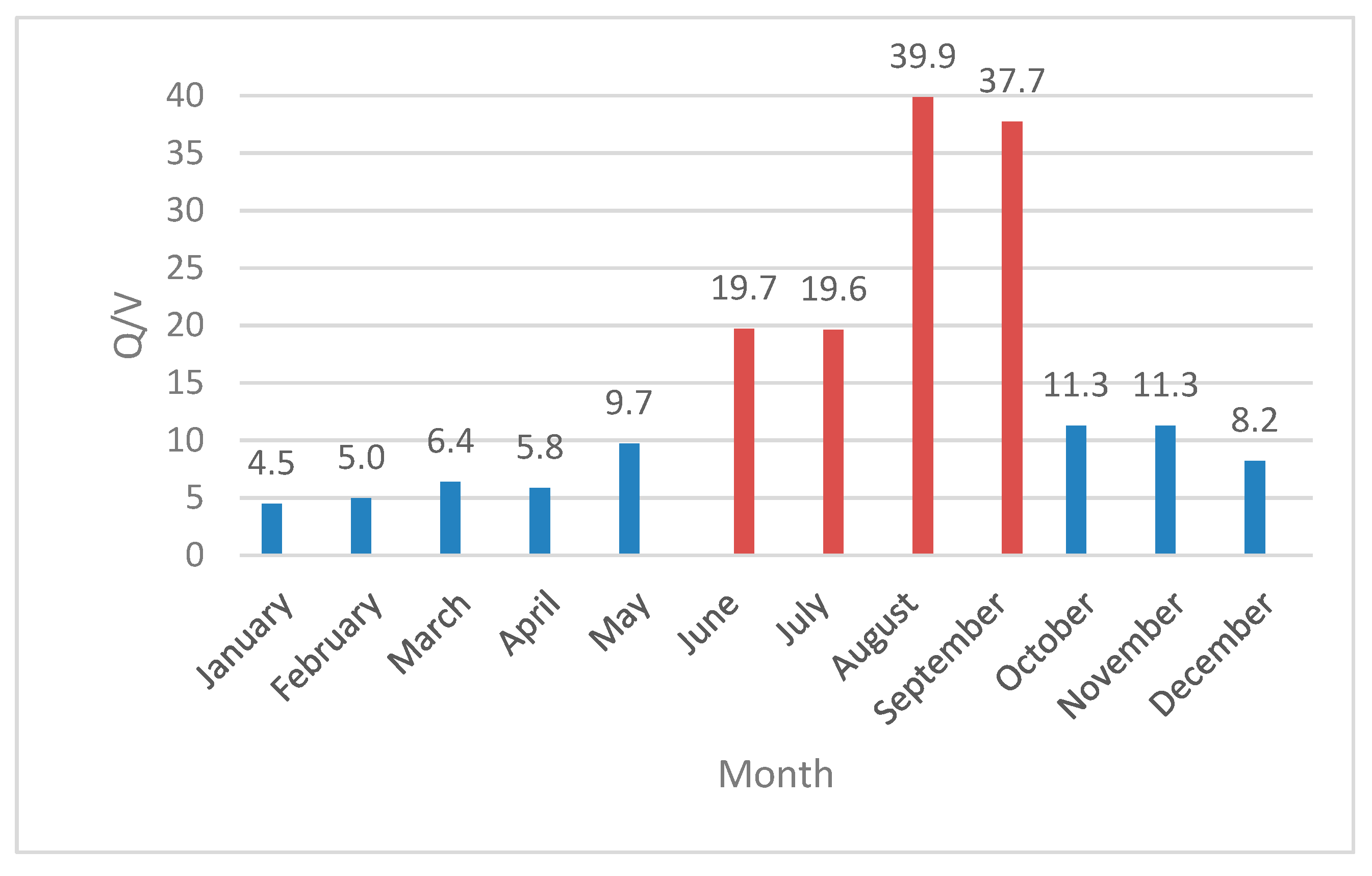
Among the different systematic approaches to identify seasons from a sample of historical flood hydrographs, the contributions of [24,25] are particularly interesting. Following its lines, and for the present the present research, the ratio α = Q/V is analyzed for all available historical flood events, in such a way that two main seasons (winter/summer) can be effectively identified, depending on the prevailing values of the ratio.
For the case study presented herein, described in detail in Section 3.2, the summer season is characterized by shorter duration flood events and, thus, larger values of the α ratio, while the winter season is characterized by longer floods and generally lower values of the α ratio.
Under the assumption that a given season presents a characteristic average ratio, for instance, αs for summer season, such a value can be estimated by means of ordinary least-squares regression through the origin (RTO) without a constant term. This regression should be performed over the family of “m” pairs (Q1, V1), (Q2, V2), …, (Qm, Vm) describing peak flows and hydrograph total volumes corresponding to “m” historical flood hydrographs that took place during the summer season. The higher the coefficient of determination for the linear regression, the more representative the αs value is for the chosen summer season. The same rule would apply for the winter season and its representative ratio value αw, with a coefficient of determination .
The best assignment of months to each season, and thus, splitting of the year into two adequate subperiods, can be attained in practice by maximizing [], regarding each of the seasons contains a minimum of 25% of the total number of historical events considered in the analysis [24].
2.2. Statistical Analysis of Input Variables
The input variables analyzed, extracted from historical records, are the following:
- Z0 = initial reservoir levels, prior to the flood event occurrence;
- Q = maximum peak of an inflow hydrograph to the reservoir;
- V = volume of the hydrograph.
With respect to the first one, Z0, descriptive statistical analyses were carried out on a monthly, seasonal, and annual basis. In each case, the empirical distribution was directly obtained from the data set. No parametric analysis has been proposed in this case, as will be later justified. Concerning (Q, V) pairs extracted from the historical flood hydrographs, a bivariate statistical analysis was performed for all selected flood events during the historical period considered. The same analysis was performed only with the summer hydrographs sample, and another one considering only the winter hydrographs. Thus, three different statistical analyses were performed. The method applied was identical in the three cases, while the samples were different.
Such methodology follows exactly the same modelling steps used in [14], including marginal distributions analysis and copula modelling.
2.2.1. Marginal Distributions
A POT (peaks over threshold) analysis [26,27,28] was performed over Q and V variables, where Q is the flow peak expressed in m3/s and V the volume expressed in 106 m3.
For each of the samples, a univariate statistical POT analysis was carried out, employing the General Pareto Distribution (GPD), which is the theoretically consistent [29,30] choice for the POT method, as in Equation (1).
where α, β, and γ are the location, scale, and shape parameter factors, respectively.
In all cases, the probability-weighted moments (PWM) method has been adopted as the parameter estimation procedure in [31,32], being an extensively used method, particularly suited for high quantile estimators [30,31,32]. Concerning goodness-of-fit tests, the Anderson–Darling test was applied for all fitted distributions. [30].
2.2.2. Copula Modeling
Floods in statistical terms are clearly a multivariate phenomenon, which requires multivariate analysis methods to adequately represent hydrological loads to infrastructures like dams [8,9,10,11,12,13].
Several properties of the flood hydrograph, apart from the flow peak, are to be taken into account for a realistic representation, including hydrograph volume, duration, and time pattern of the hydrograph. All of them actually affect spillway operation in dam routing. For the purposes in this research, a bivariate statistical analysis was performed considering the most relevant variables Q and V, thus accounting for the empirical statistical dependence observed between both variables.
Copula modelling comprises the analysis of the empirical statistical dependence among the two variables involved (Q and V), the copula selection, copula fitting, and finally a goodness-of-fit assessment. Details of the procedure applied herein can be found in [14].
The degree of statistical dependence between both variables Q and V was quantified through analytical methods [33]. In particular, γ-Pearson, ρ-Spearman, and τ-Kendall statistics were computed for each of the three samples analyzed.
Concerning copula selection, an interesting study assessing limitations, properties, and key aspects for a best choice can be found in [34]. The tested copulas herein were extreme value copulas [9,11,34]. More precisely, the ones that were applied and compared in this research were Gumbel, Galambos, and Hüsler-Reiss (H-R). Table 1 shows the characteristic function defining each of them.
With respect to the copula fitting procedure, several methods based in ranges were used herein: the maximum pseudo-likelihood method (MPL), Kendall’s inversion, and Spearman’s methods have been selected. In all three cases, the parameter estimation does not depend on marginal distribution properties [35].
Concerning the copula goodness-of-fit assessment, there are a wide variety of tests available in the literature, both graphic and analytical ones [36]. The Cramér-von Mises statistic (Sn based on the empirical copula) shows satisfactory behavior for all copula models, making it possible to differentiate among extreme value copulas [37].
The Sn statistic can be written as Equation (2).
where Sn is the Cramer-von Mises statistic, and A is the Pickands dependence function. An and are, respectively, non-parametric and parametric estimators of A, which are calculated following strictly the expressions in [37].
Also, it is important to calculate the p-value associated to the goodness-of-fit test to formally assess whether the selected model is suitable. The p-value was obtained through a parametric bootstrap-based procedure, validated in [37,38].
The tail dependence coefficient has been also calculated for each of the tested copulas [33]. The comparison between empirical and theoretical values indicates the ability of the different copulas tested to satisfactorily reproduce the statistical dependence observed in the distribution tail. Table 2 shows the theoretical values of the tail dependence coefficient. The empirical estimators of this parameter have been computed according to [39].
2.3. Synthetic Hydrographs Generation
The stochastic approach proposed herein is focused on the generation of flood inflow hydrographs to the reservoir under study. Three ensembles of synthetic hydrographs were generated (one for winter, one for summer, and another one for the whole year). The size of each ensemble was 50,000. The procedure used a Monte Carlo generation of 50,000 pairs (Q, V) using estimated marginal distributions and selected copulas. Then, a definition of a theoretical time pattern for the synthetic hydrograph, corresponding to each pair of values (Q, V), was introduced. To do so, a gamma-shaped hydrograph was adopted, which is a classic approximation in hydrology proposed by mid-twentieth century investigators [40,41], and provides an ideal representation of the most usual cases found in the observed hydrographs. It contemplates a rising branch until reaching the peak, followed by a more gradual decrease and more extended period in time (Equation (3)). Basically, the gamma shape results from the convolution of an instantaneous unit hydrograph of a cascade of n equal linear reservoirs [40].
Although there exists a variety of methods to estimate the parameters of this hydrograph, a practical procedure to determine it has been adopted, as proposed by [42,43]. Time to the peak is firstly calculated by using the simplest triangular formulation of the hydrograph, and then both parameters of the gamma function are estimated. Equation (3) shows the theoretical resulting expression.
where , and k,n must satisfy and .
2.4. Dam Routing
The assessment of the hydrological safety of the dam as well as the accurate evaluation of downstream flooding risks are not only conditioned by the probabilistic definition of inflows to the reservoir. Dam routing obviously plays a crucial role, as outflow hydrographs over the spillway and maximum floodwater levels reached in the reservoir clearly depend on the dam routing process. Therefore, the hydraulic behavior of the spillway together with the previous reservoir surface level at the initiation of the flood event (Z0) are key factors to take into account in the simulations. Although the first one is essentially deterministic, the second factor clearly requires a probabilistic description.
Different authors have presented dam routing applications considering Z0 as a random variable [7,44,45], as it is clear that those levels can significantly fluctuate throughout the year. This is due to a variety of reasons such as randomness of natural flood events and dam operation rules. In the case study presented herein (spillway without gates), such rules basically included water supply operations to satisfy downstream irrigation demands along the year, ecological flow maintenance, and freeboard management policies preventing dam hydrological risks. In the context of the Monte Carlo simulation to be performed, the natural option to introduce Z0 in the stochastic analysis would be to assign random values drawn from the empirical distribution of historical Z0 registers. This was the criteria adopted in this research, following the lines of [7,44,45]. In this case, though, empirical distributions were obtained previously for each of the seasons considered when the Monte Carlo simulation was performed on seasonal basis. When seasonality is ignored, Monte Carlo simulations on an annual basis are likely to include many scenarios involving values of (Z0, Q, V) that are not realistic. For instance, certain typical summer flash floods would be dam-routed, assuming an unrealistic previous water level Z0, at least in a probabilistic sense. This concern is a key aspect affecting results, and in particular distributions of output variables such as MWRL (maximum water reservoir level reached during flood dam routing) and MO (maximum outflow discharge in the spillway during flood dam routing). In fact, such distributions should be affected not only by the different nature of seasonal floods (as explained in Section 2.1), but also by the different expected Z0 values according to observed seasonal empirical frequency distributions.
Previous modelling step 2.3 provides a wide collection of design synthetic flood hydrographs (DFHs), preserving observed empirical statistics and dependencies between both selected variables Q and V. The Monte Carlo approach provides three samples of 50,000 DFHs, each one corresponding to summer season hydrographs, winter season hydrographs, and for the whole year hydrographs.
The routing effect of a given dam with single crested spillway is evaluated through the use a practical dam routing scheme. The basic equation is the following Equation (4):
where S(t) represents the volume of water stored in the reservoir at time t, and I(t) is the inflow expressed in m3/s, while Q (t, S) is the outflow discharge over the spillway. If the reservoir storage capacity S is defined as a function of the water surface level H, the area of the water surface can be derived as A = dS/dH, and the hydraulic water balance equation can be written in the following form (Equation (5)):
At a given time t, the outflow from the reservoir is a function of the reservoir water level H and the geometry and hydraulic operation of the spillway. Under the simple hypothesis of a free fixed crest of known length L, the outflow can be evaluated through Equation (6):
where Q is the outflow, CD is the discharge coefficient, L is the spillway length, and h is the water height over the spillway fixed crest.
The practical application of dam routing for a given synthetic flood hydrograph requires a previous definition of the initial water level in the reservoir [7,44,45]. The values used in the simulations were random following the empirical distributions observed in each of the corresponding seasons under consideration (summer, winter, and whole year). Thus, statistical independence of initial reservoir water levels with respect the DHFs was assumed herein, although different empirical distributions were used in each case, depending on the season under consideration. Practical solution of Equations (4) and (5) were discussed long ago [46], including analytical approaches under a hypothesis of a power function representing the storage–outflow discharge relationship. Concerning numerical approaches, which are usually more convenient, there are many different strategies found in the literature [46,47,48,49,50]. Authors in [48] discuss the robustness of several numerical methods for the solution of the dam routing equation. One of the most straight-forward techniques resorts to the trapezoidal rule to approximate Equation (5), resulting in Equation (7):
where Sj represents the reservoir storage at the start of interval j, and Sj+1 is the storage at the end of the time interval. Ij, Ij+1 are respective values of inflow at the start and end of the time interval, and Qj and Qj+1 are the spillway discharges at the beginning and end of the interval.
Other more robust numerical methods are proposed in the literature. The Laurenson-Pilgrim method, the fourth-order Runge-Kutta method, and the fixed order Cash-Karp method can be outlined. For the purposes of the research presented herein, the simpler trapezoidal rule Equation (7) was adopted, which in fact yielded negligible differences with respect to the Runge-Kutta algorithm for small Dt time increments.
For each and every one of the synthetic events considered, dam routing provides an output hydrograph with a maximum outflow (MO), a maximum water level reached in the reservoir during the process (MWRL), and a parametric index evaluating routing coefficient η, defined as the ratio between the outflow hydrographs and the inflow flood peak discharge [47,48,49,50].
Therefore, and after processing all the synthetic hydrographs of the three ensembles, cumulative distributions of the maximum water level reached in the reservoir, maximum outflow (output hydrograph peak), and coefficient η were obtained, providing solid bases for reliable quantile estimations at given return periods, as well as quantitative evaluation of the effect of introducing seasonality in the statistical analysis.
3. Case Study
3.1. Basic Descriptors of the Catchment
The Martin river catchment, controlled by Cueva Foradada dam, has been selected as the case study. Martin river is a tributary of Ebro river, with a total length of 98 km until the dam and an average slope of 0.014. The catchment area is 600 km2 until the dam location. The upper Martin river catchment belongs to a moderate mountain region in a continental zone, with an average annual cumulative precipitation close to 500 mm/year, with negligible snow occurrence. The mountain range has peaks over 1500 m where the Martin river is born. The lower part of the catchment downstream from the dam exhibits precipitation rates under 300 mm/year, turning into a mild, semiarid Mediterranean climatic context [51]. Figure 1 shows the location of the catchment, while Figure 2 presents an aerial view of the reservoir and the dam, equipped with a fixed crest spillway of length 110 m. The maximum reservoir storage capacity is 22.08·106 m3, producing a surface water area of 2.3·106 m2. The reservoir is used to satisfy local irrigation demands on the downstream plain closer to Ebro river.
3.2. Data Set
The historical hydrographs analyzed in this research were from 1964–2018. A total of 214 flood events were selected, each one of them defined in terms of an inflow hydrograph to the reservoir. Figure 3 presents one of the events, illustrating the relevant variables derived from the flood hydrograph.
The average annual flow rate of Martin river was very low, although it showed sudden increments originated by high intensity precipitation events. The most characteristic ones were summer events of relatively short duration and high rainfall rates, usually associated to convective precipitation events that produced rapidly increasing river discharges over a short period of time. They resulted in flash floods with characteristic steep rising limbs in the hydrographs and important peak flows (Q). These events usually presented small lag times and typically took place during late spring and summer months. On the other hand, more persistent rainfall derived from frontal systems usually occurred along the rest of the year, eventually producing floods with longer duration (i.e., several days) and more significant volumes (V). From this point of view, it can be initially assumed the existence of two main flood typologies that are identified hereafter as winter floods and summer floods [52].
According to the qualitative description of summer vs winter typical floods, the α ratio previously introduced in Section 2.1 becomes useful for practical identification of seasons. Summer floods should be expected to generally produce higher α-ratios, while winter floods should in principle yield to lower α values. This α-ratio was computed for the complete set of selected floods. The resulting monthly averaged values are presented in Figure 4.
According to the procedure described in Section 2.1, ordinary least-squares regression through the origin (RTO) without constant term was applied to (Q, V) pairs, with month assignments arranged in several combinations of two subperiods or consecutive seasons. Table 3 shows results of the estimated values.
Figure 5 presents the scatterplot of pairs (Q, V) and the corresponding optimal regressions maximizing regression efficiencies . This optimal value was achieved when the year was divided into the following two periods: June to September (summer period) and October to May (winter period). This result was expected, after the monthly statistics already shown in Figure 4.
Table 4 presents some relevant empirical statistics for the complete sample of 214 hydrographs and also for the subsamples corresponding to each of the two seasons identified.
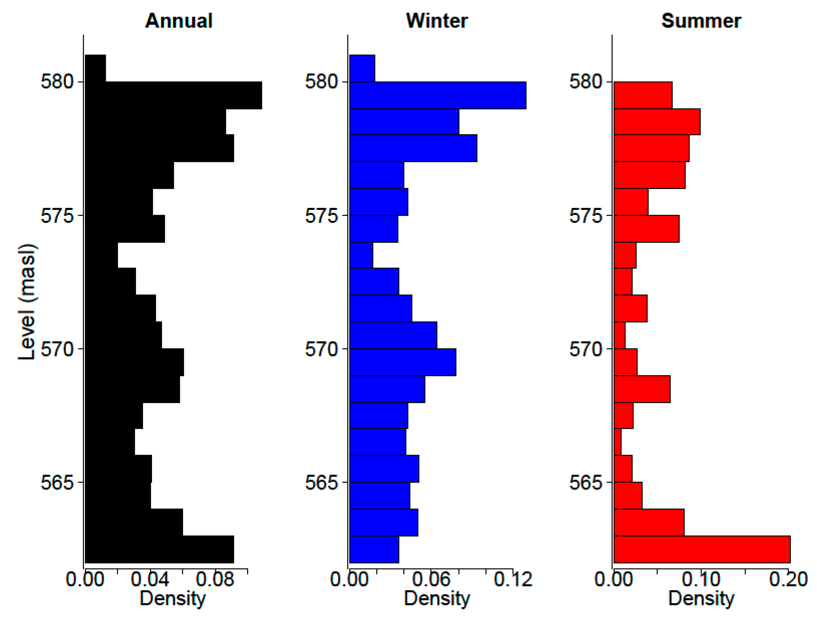
According to the two subperiods established, the empirical distribution of Z0 values has been obtained for each one of them. Figure 6 shows the empirical frequency distribution of the reservoir water level for each case (data provided by the Confederación Hidrográfica del Ebro (CHE)).
4. Results
4.1. Marginal Distributions of Q and V
The procedure described in Section 2.2.1 has been applied to perform the flood frequency analysis for flow peaks (Q) at the river Martin, using data from gauge station Alcaine. The thresholds used for each of the samples were estimated using the mean residual life plot methodology [53]. The resulting estimations are the a values reported in Table 5. The sample to be analyzed included a total of 214 values of Q, representing peak flows values of each of the selected flood hydrographs during the period 1964 to 2018. Statistical analysis of variable V, representing the hydrograph volume (106 m3), was also performed according to the same hypothesis detailed in Section 2.2.1. The resulting fitted distributions are presented in Figure 7.
The cumulative distribution function in Figure 7 provides a direct answer to practical estimation of the peak flow Q expected for a given return period T, regardless of the season in which it occurs, that is, considering annual flood frequency regime. To do so, Equation (8) should be applied [54]:
where Q is the peak flow value corresponding to return period T, λ is the average number of peaks per year in the sample, and F(Q) is the fitted theoretical cumulative distribution function. In case of applying this classical annually based analysis, any aspect concerning seasonality is being completely ignored.
The same procedure previously described, can be also applied with sub-yearly samples, in order to assess estimation of seasonal flood frequencies, that is, flood frequencies referred exclusively to events taking place in the intra-annual period under consideration (either summer or winter, in this case). Table 5 presents the estimated parameters GPD after applying the PWM method, for the different samples analyzed, including the referred analysis of Figure 7, which was performed for annual flood frequency regime. For all distributions fitted, the Anderson-Darling test was applied, yielding to no rejection of the hypothesis that the given sample of data is actually drawn from GPD theoretical distribution.
Figure 8 and Figure 9 show resulting GPDs fitted to seasonal samples, including both the flow peaks (Q) and the hydrographs volumes (V).
These probability distributions estimate, in practice, the expected peak flow value (or hydrograph volume) associated to an assigned return period, given that the flood event occurs in the intra-annual period under consideration.
It is interesting to remark that distributions in Figure 8 and Figure 9 clearly reflect the qualitative aspect previously discussed about the different nature and characteristics of summer floods versus winter floods. For a given return period, flow peaks in Figure 9 (summer floods) were indeed significantly higher than those derived from Figure 8 (winter floods). This is exactly as expected, in accordance with known seasonal differences concerning hydrological dynamics of the catchment. Conversely, hydrograph volumes estimated for a given T are clearly larger in the winter season (Figure 8), as compared to those derived from Figure 9.
4.2. Copula Modeling
The results of (Q, V) bivariate analysis based on copula modelling resulted from the application of the method described in Section 2.2.1, comprising the following steps: analysis of the observed statistical dependence among variables, copula selection, copula fitting, and goodness-of-fit assessment. The procedure is carried out exactly in the same manner for each of the three samples analyzed herein (summer season, winter season, and whole year period), following the modelling steps in [14] where further details about copula modelling can be found.
Table 6, Table 7 and Table 8 present results obtained concerning estimation of characteristic copula values for the chosen family of extreme value copulas (i.e., Gumbel, Galambos, and Husler-Reiss copulas). The copula parameter θn estimates n and was obtained through the methods of statistical inference based in ranges, already mentioned in Section 2.2.2. Table 6, Table 7 and Table 8 also include the p-value as well as the Cramer-von Mises statistic proposed by [55]. For each of the tables, the best copula estimation method is highlighted in bold according to the goodness-of-fit tests computed.
The best behavior was exhibited by the Husler-Reiss copula for all cases. As explained in Section 2.2.2, in order to further contrast suitability of the copulas under study, the dependence coefficient of the upper tail of the distribution was analyzed. To do so, theoretical and empirical values of the statistic λU were compared. These are presented in Table 9 and Table 10, respectively. The empirical estimates have been calculated using the estimator proposed by [39].
From values presented in Table 9 and Table 10, it can be concluded that theoretical and empirical estimates of λU values were very similar, indicating a satisfactory behavior of the right upper tail of the distribution. The values highlighted in bold are the ones that better fit the empirical estimators of the samples, which were copula Husler-Reiss in all cases.
4.3. Monte Carlo Simulation
Synthetic ensembles of 50,000 pairs (Q, V) have been generated via Monte Carlo simulation, following the generation scheme mentioned in Section 2.3. As a result of the process, three long families of synthetic pairs were obtained: (Qa, Va) for annual period, (Qw, Vw) for winter season, and (Qs, Vs) for summer season.
Figure 10 presents a scatter plot of 50,000 values generated from each of the three copulas fitted. Each of the dots in Figure 10 is linked to a synthetic, gamma-shaped hydrograph, with parameters n and k directly obtained from the given pair (Q, V) following the criteria described in Section 2.3. As a consequence, a family of 50,000 synthetic hydrographs was available for each of the periods (i.e., winter, summer, and annual periods). These collections of synthetic hydrographs satisfactorily preserved statistics of the main characteristics observed in historical records, including peak flow, volume, and statistical dependence between both. This applied for each of the seasons and also for the historical hydrographs observed, regardless of the season during which they took place. They can be effectively used as hydrological loads for the Cueva Foradada reservoir in order to assess hydrological safety of the dam and other issues of interest, such as optimal management of the dam, freeboards, infrastructure design improvements, risk evaluation, and so forth.
4.4. Reservoir Dam System Routing
Figure 6 presents the observed Z0 frequency distributions for the winter season, summer season, and for the whole year in the Cueva Foradada reservoir. As expected, important differences can be identified between them. When the Monte Carlo scheme was performed on an annual basis, the ensemble of synthetic hydrographs was used with no consideration of the season in which they occurred. These hydrographs were dam routed using Z0 values randomly taken from the empirical annual distribution (black frequency histogram in Figure 6), and thus, with no concern about seasons. An analogous procedure was applied using the other two ensembles (summer and winter floods), using the corresponding empirical Z0 distribution in Figure 6.
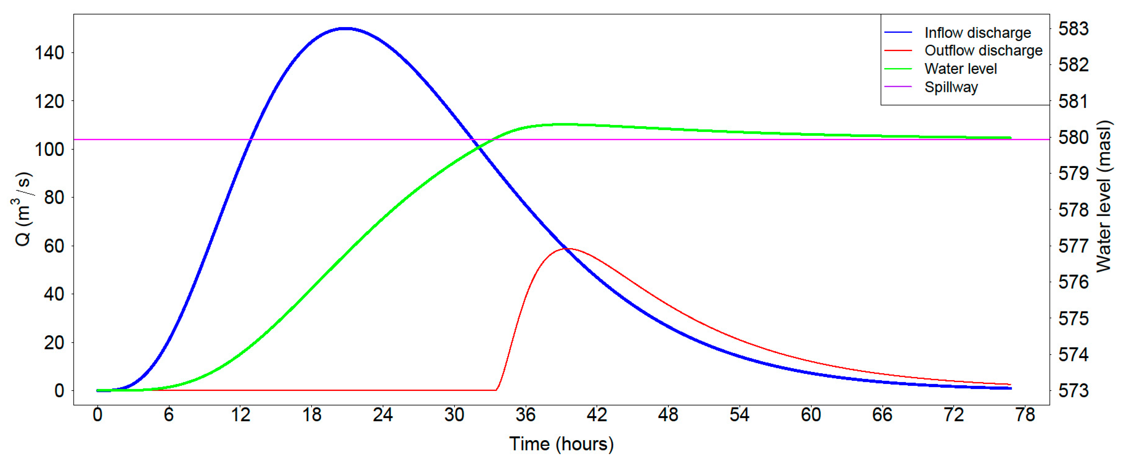
A total of 150,000 simulations were performed: 50,000 (summer), 50,000 (winter), and 50,000 (annual), all resulting from dam routing process equations described in Section 2.4. For every one of them, both output variables MWRL and MO were obtained. Figure 11 shows an example of the dam routing application to one synthetic hydrograph.
For each of the season ensembles, the application of a simple plotting position, Equation (9), provides MWRL and MO frequency curves.
In Equation (9), r is the order of each of the values, c is a coefficient, and n is the size of the sample. c value is taken equal to 0.44 according to [56].
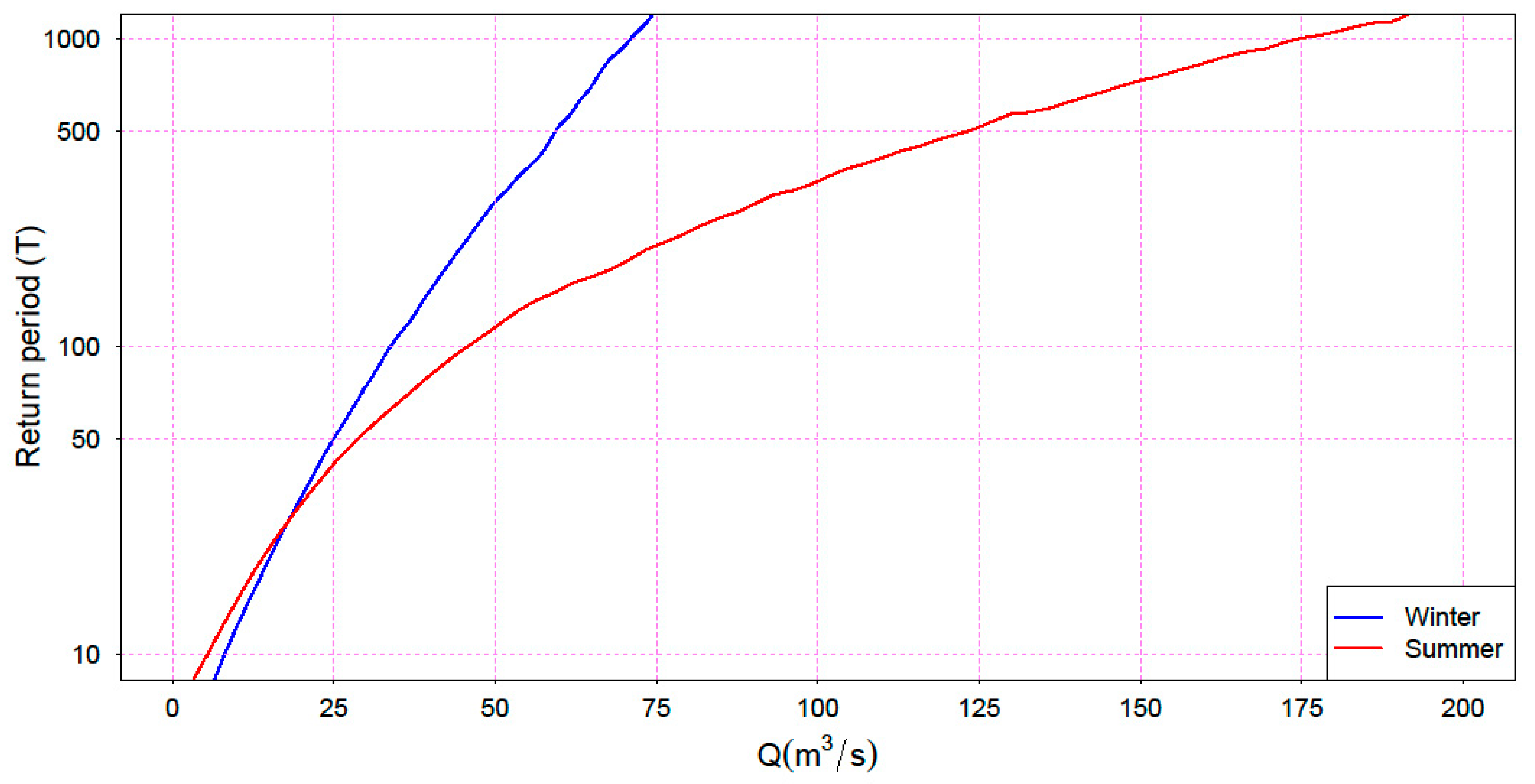
Figure 12 shows results obtained for variable MWRL, while Figure 13 shows the results corresponding to variable MO.
CDFs plotted in red and blue (Figure 12 and Figure 13) provide probability estimations for both objective variables (MWRL and MO), given that the flood event occurs in either summer or winter, respectively. As expected, summer events yielded larger values of both MWRL and MO, as a consequence of the intense convective storms usually taking place during months of June, July, August, and September. It should be noted, though, that for low return periods (ordinary floods), both MWRL and MO quantiles are expected to be larger for winter season. In particular, this is true for T < 30 years. This fact is associated to situations when Z0 is close to the spillway crest level. While this never occurs during summer season, it is more likely to occur during winter months, and can effectively give rise to outflows in the spillway during ordinary floods. Concerning the index coefficient η, defined as the ratio between the outflow hydrographs and the inflow flood peak discharge, certain differences were found between seasons. Table 11 shows basic statistics for the η coefficient after Monte Carlo simulations. It should be noted that attenuation of the peak was more efficient during summer months, in a statistical sense. During the summer season, there is usually a larger available storage capacity in the reservoir. On top of that, the frequency of intense summer floods is characterized by fast hydrological responses, more concentrated in time, resulting in steep rising limbs of the hydrographs. Therefore, it should be expected that during summer flood events, peak inflow frequently occurs while the reservoir has not reached 100% storage capacity. As a consequence, the η coefficient tends to be lower for the summer season when compared to values obtained for winter floods.
It is of practical interest for the hydrological risk assessment to obtain quantile estimations of maximum expected MWRL and MO values for selected return periods, regardless of the season in which flood is taking place, based on the seasonal stochastic analysis previously performed. Thus, the idea is to infer the MWRL and MO frequency distributions at an annual time scale, benefiting from the more realistic approach performed on the seasonal time scale. The annual cumulative distribution can be obtained as the product of the seasonal cumulative distribution functions, under the assumption of statistical independence among different seasons [15,57]. This assumption has been adopted in related recent studies [23,24]. Following those lines, it is possible to infer the MWRL and MO CDFs for the annual flood frequency regime, based on the seasonal stochastic approaches (Figure 14 and Figure 15). The modelling framework proposed herein allows to quantify the seasonality effect because the Monte Carlo approach is also performed on a classical annual basis. For this purpose, and additional ensemble of 50,000 synthetic hydrographs were dam routed. In this case, such synthetic hydrographs had no consideration of the season in which they occurred. They were routed using Z0 values randomly taken from the annual empirical distribution (Figure 6), with no concern about seasons. Therefore, it should be remarked that resulting CDFs plotted in black (Figure 14 and Figure 15) were obtained from a computational scheme that completely ignored seasonality. In other words, bivariate statistical analysis of Q and V distributions was performed, regardless of the season in which the flood event occurred. On the other hand, water levels in the reservoir prior to flood occurrence were random values drawn from the empirical distribution of Z0 along the year (Figure 6), also ignoring seasonal trends.
Figure 14 and Figure 15 show the resulting frequency distributions. For the case study under consideration, it can be observed that the classical approach ignoring seasonality properties in the analysis provided quantiles with small differences from the seasonal approach, at least for return periods under T = 125 years. For larger T values, though, a degree of underestimation was observed, which was more significant as return periods increased. In particular, for T = 1000 years, the MWRL was underestimated by 26 cm (Table 12), equivalent to 402000 m3, while the maximum outflow was underestimated by 29% (Table 13). Therefore, ignoring the seasonal statistical properties yields a quantile underestimation that might be relevant in the context of hydrological risk evaluation.
5. Conclusions
The modelling framework proposed herein allows to estimate MWRL and MO, expected for an assigned return period T, for annual flood frequency regime. In other words, final quantiles are estimated for both selected variables, independently of the season in which flooding occurs. The method is based on the stochastic analysis of seasonal floods, which are described in terms the hydrograph peak (m3/s) and the hydrograph volume (106 m3), incorporating in the analysis observed dependencies between Q and V through copula modelling approach. Previous reservoir levels at the initiation of the flood event are also incorporated on seasonal basis through the empirical distribution observed in the Cueva Foradada reservoir.
The resulting CDFs for seasonal MWRL and MO are consistent with known differences between the historical flood events during different periods of the year. The annual flood frequency distribution is obtained as the product of the seasonal cumulative distribution functions, under the assumption of statistical independence among different seasons.
On the other hand, a classical approach is also performed on an annual basis and ignoring the seasonal statistical properties and of variables Q, V, and Z0 in any of the modelling steps. We find that seasonality consideration induces higher values of maximum expected MWRL and MO values for a given return period, in particular for T > 125. This approach is more realistic than the classical annual analysis due to its ability to provide an improved multivariate representation of the known qualitative properties of summer floods and winter floods. The use of the specific empirical seasonal distributions for Z0 yields more reliable estimates of variables resulting from dam routing (i.e., MWRL and MO). Results outline the importance of considering seasonality when dealing with flood management and, more particularly, hydrological dam safety.
For the case of the river Martin catchment, controlled by the Cueva Foradada dam, rainfall regime characteristics produce maximum inflow peaks to the reservoir during the summer season. Thus, the maximum expected values of MWRL and MO are generally larger for summer, at least when extraordinary floods are considered. However, for ordinary floods (lower T values), winter events produce larger expected quantiles of both MWRL and MO, mainly due to the higher probability of having the reservoir close to its maximum capacity. This conclusion clearly arises from the statistical approach based on seasons, providing a more realistic bivariate modeling of variables (Q, V) for each season, while making use of a Z0 empirical distribution also obtained specifically for each of the seasons.
Ignoring seasonality effects in the statistical analysis yields significant underestimations of maximum outflows in the spillway during flood events (MO). The results obtained for the case study of Foradada Dam in river Martin (Spain) indicate MO underestimations of 18% for T = 500 years and 29% for T = 1000 years. For return periods under 125 years, quantile estimations are not significantly affected by seasonal trends. Although it should be noted that slight overestimations result from ignoring seasonality.
Concerning maximum flood water levels reached in the reservoir (MWRL), also underestimation of quantiles for T > 125 years is observed, resulting from the classical annual flood frequency analysis. Nevertheless, theses underestimates are not so significant as those of (MO). Ignoring seasonality in the statistical analysis, the underestimation of reservoir maximum storage during flood occurrence is approximately 160,000 m3 (T = 500 years) and 402,000 m3 (T = 1000 years). For lower return periods (T < 125), no significant seasonality effect is observed in this case.
The approach presented herein represents a convenient framework to assess optimization freeboard policies, as it makes use of the Z0 empirical frequency distributions. Different management strategies concerning freeboards policies yield to changes in Z0 distributions, which might be introduced in the simulation scheme proposed herein, in order to assess potential changes in variables affecting downstream flooding risk and hydrological dam safety.
The methodology described presents several limitations derived from various hypotheses introduced, which should be outlined. Firstly, the already mentioned issue concerning the seasonal statistical independence hypothesis would require further research. On the other hand, the question concerning hydrograph time pattern, it is a known fact that real hydrographs actually present a variety of patterns, eventually including more than one peak [48], while a single peaked hydrograph is being assumed herein, following a Nash type pattern [41].
Finally, the stochastic approach developed in this research is stationary; thus, it does not incorporate any climate change projection. In [58,59], evidence of climate change effects on floods is reported. This concern introduces larger uncertainty when high return periods T are considered. Such studies point out future changes in flood regimes affecting not only frequency and magnitude of floods, but also a shift in their timing, which might increase the seasonality effects in statistical terms [60,61,62,63].
Author Contributions
Conceptualization, J.Á.A. and R.G.-B.; Data curation, J.Á.A.; Formal analysis, J.Á.A. and R.G.-B.; Investigation, J.Á.A. and R.G.-B.; Methodology, J.Á.A. and R.G.-B.; Project administration, R.G.-B.; Resources, J.Á.A.; Software, J.Á.A.; Supervision, R.G.-B.; Validation, J.Á.A. and R.G.-B.; Visualization, J.Á.A.; Writing—original draft, J.Á.A. and R.G.-B.; Writing—review & editing, R.G.-B. All authors have read and agreed to the published version of the manuscript.
Funding
This research received no external funding.
Acknowledgments
The authors wish to acknowledge support from Confederación Hidrográfica del Ebro.
Conflicts of Interest
The authors declare no conflicts of interest.
References
- Blazkova, S.; Beven, K. Flood frequency estimation by continuous simulation of subcatchment rainfalls and discharges with the aim of improving dam safety in a large basin in the Czech Republic. J. Hydrol. 2004, 292, 153–172. [Google Scholar] [CrossRef]
- Mo, C.; Mo, G.; Yang, Q.; Ruan, Y.; Jiang, Q.; Jin, J. A quantitative model for danger degree evaluation of staged operation of earth dam reservoir in flood season and its application. Water Sci. Eng. 2018, 11, 81–87. [Google Scholar] [CrossRef]
- Liu, Z.; Xu, X.; Cheng, J.; Wen, T.; Niu, J. Hydrological risk analysis of dam overtopping using bivariate statistical approach: A case study from Geheyan Reservoir, China. Stoch. Environ. Res. Risk Assess. 2018, 32, 2515–2525. [Google Scholar] [CrossRef]
- King, L.M.; Schardong, A.; Simonovic, S.P. A Combinatorial Procedure to Determine the Full Range of Potential Operating Scenarios for a Dam System. Water Resour. Manag. 2019, 33, 1451–1466. [Google Scholar] [CrossRef]
- Chen, J.; Zhong, P.; Wang, M.; Zhu, F.; Wan, X.; Zhang, Y. A risk-based model for real-time flood control operation of a cascade reservoir system under emergency conditions. Water 2018, 10, 167. [Google Scholar] [CrossRef] [Green Version]
- Gabriel-Martin, I.; Sordo-Ward, A.; Garrote, L.; Granados, I. Hydrological Risk Analysis of Dams: The Influence of Initial Reservoir Level Conditions. Water 2019, 11, 461. [Google Scholar] [CrossRef] [Green Version]
- Gabriel-Martin, I.; Sordo-Ward, A.; Garrote, L.; Castillo, L.G. Influence of initial reservoir level and gate failure in dam safety analysis. Stochastic approach. J. Hydrol. 2017, 550, 669–684. [Google Scholar] [CrossRef]
- Requena, A.I.; Mediero, L.; Garrote, L. A bivariate return period based on copulas for hydrologic dam design: Accounting for reservoir routing in risk estimation. Hydrol. Earth Syst. Sci. 2013, 17, 3023–3038. [Google Scholar] [CrossRef] [Green Version]
- Mediero, L.; Jiménez-Álvarez, A.; Garrote, L. Design flood hydrographs from the relationship between flood peak and volume. Hydrol. Earth Syst. Sci. 2010, 14, 2495–2505. [Google Scholar] [CrossRef] [Green Version]
- Goodarzi, E.; Mirzaei, M.; Shui, L.T.; Ziaei, M. Evaluation dam overtopping risk based on univariate and bivariate flood frequency analysis. Hydrol. Earth Syst. Sci. Discuss. 2011, 8, 9757–9796. [Google Scholar] [CrossRef]
- De Michele, C.; Salvadori, G.; Canossi, M.; Petaccia, A.; Rosso, R. Bivariate statistical approach to check adequacy of dam spillway. J. Hydrol. Eng. 2005, 10, 50–57. [Google Scholar] [CrossRef]
- Volpi, E.; Fiori, A. Design event selection in bivariate hydrological frequency analysis. Hydrol. Sci. J. 2012, 57, 1506–1515. [Google Scholar] [CrossRef]
- Rizwan, M.; Guo, S.; Yin, J.; Xiong, F. Deriving Design Flood Hydrographs Based on Copula Function: A Case Study in Pakistan. Water 2019, 11, 1531. [Google Scholar] [CrossRef] [Green Version]
- Aranda, J.A.; García-Bartual, R. Synthetic hydrographs generation downstream of a river junction using a copula approach for hydrological risk assessment in large dams. Water 2018, 10, 1570. [Google Scholar] [CrossRef] [Green Version]
- Waylen, P.; Woo, M. Prediction of annual floods generated by mixed processes. Water Resour. Res. 1982, 18, 1283–1286. [Google Scholar] [CrossRef]
- Villarini, G.; Smith, J.A. Flood peak distributions for the eastern United States. Water Resour. Res. 2010, 46. [Google Scholar] [CrossRef] [Green Version]
- Smith, J.A.; Villarini, G.; Baeck, M.L. Mixture Distributions and the Hydroclimatology of Extreme Rainfall and Flooding in the Eastern United States. J. Hydrometeorol. 2011, 12, 294–309. [Google Scholar] [CrossRef]
- Strupczewski, W.G.; Kochanek, K.; Bogdanowicz, E.; Markiewicz, I. On seasonal approach to flood frequency modelling. Part I: Two-component distribution revisited. Hydrol. Process. 2012, 26, 705–716. [Google Scholar] [CrossRef]
- Collins, M.J.; Kirk, J.; Pettit, J.; Degaetano, A.T.; Sam Mccown, M.; Peterson, T.C.; Means, T.N.; Zhang, X. Annual floods in New England (USA) and Atlantic Canada: Synoptic climatology and generating mechanisms. Phys. Geogr. 2014, 35, 195–219. [Google Scholar] [CrossRef]
- Vormoor, K.; Lawrence, D.; Schlichting, L.; Wilson, D.; Wong, W.K. Evidence for changes in the magnitude and frequency of observed rainfall vs. snowmelt driven floods in Norway. J. Hydrol. 2016, 538, 33–48. [Google Scholar] [CrossRef]
- Iacobellis, V.; Fiorentino, M.; Gioia, A.; Manfreda, S. Best fit and selection of theoretical flood frequency distributions based on different runoff generation mechanisms. Water 2010, 2, 239–256. [Google Scholar] [CrossRef]
- de Michele, C.; Salvadori, G. On the Derived Flood Frequency Distribution: Analytical Formulation and the Influence of Antecedent Soil Moisture Condition. J. Hydrol. 2002, 262, 245–258. [Google Scholar] [CrossRef]
- Baratti, E.; Montanari, A.; Castellarin, A.; Salinas, J.L.; Viglione, A.; Bezzi, A. Estimating the flood frequency distribution at seasonal and annual time scales. Hydrol. Earth Syst. Sci. 2012, 16, 4651–4660. [Google Scholar] [CrossRef] [Green Version]
- Fischer, S.; Schumann, A.; Schulte, M. Characterisation of seasonal flood types according to timescales in mixed probability distributions. J. Hydrol. 2016, 539, 38–56. [Google Scholar] [CrossRef]
- Yan, L.; Xiong, L.; Ruan, G.; Xu, C.-Y.; Yan, P.; Liu, P. Reducing uncertainty of design floods of two-component mixture distributions by utilizing flood timescale to classify flood types in seasonally snow covered region. J. Hydrol. 2019, 574, 588–608. [Google Scholar] [CrossRef]
- Madsen, H.; Rasmussen, P.F.; Rosbjerg, D. Comparison of annual maximum series and partial duration series methods for modeling extreme hydrologic events: 1. At-site modeling. Water Resour. Res. 1997, 33, 747–757. [Google Scholar] [CrossRef]
- Claps, P.; Laio, F. Can continuous streamflow data support flood frequency analysis? An alternative to the partial duration series approach. Water Resour. Res. 2003, 39. [Google Scholar] [CrossRef] [Green Version]
- Lang, M.; Ouarda, T.; Bobée, B. Towards operational guidelines for over-threshold modeling. J. Hydrol. 1999, 225, 103–117. [Google Scholar] [CrossRef]
- Balkema, A.A.; de Haan, L. Residual Life Time at Great Age. Ann. Probab. 1974, 2, 792–804. [Google Scholar] [CrossRef]
- Ferreira, A.; de Haan, L. On the block maxima method in extreme value theory: PWM estimators. Ann. Stat. 2015, 43, 276–298. [Google Scholar] [CrossRef] [Green Version]
- Dupuis, D.J. Estimating the probability of obtaining nonfeasible parameter estimates of the generalized pareto distribution. J. Stat. Comput. Simul. 1996, 54, 197–209. [Google Scholar] [CrossRef]
- Hosking, J.R.M.; Wallis, J.R.; Wood, E.F. Estimation of the Generalized Extreme-Value Distribution by the Method of Probability-Weighted Moments. Technometrics 1985, 27, 251–261. [Google Scholar] [CrossRef]
- Serinaldi, F. Analysis of inter-gauge dependence by Kendall’s τK, upper tail dependence coefficient, and 2-copulas with application to rainfall fields. Stoch. Environ. Res. Risk Assess. 2008, 22, 671–688. [Google Scholar] [CrossRef]
- Dupuis, D.J. Using copulas in hydrology: Benefits, cautions, and issues. J. Hydrol. Eng. 2007, 12, 381–393. [Google Scholar] [CrossRef]
- Kim, G.; Silvapulle, M.J.; Silvapulle, P. Comparison of semiparametric and parametric methods for estimating copulas. Comput. Stat. Data Anal. 2007, 51, 2836–2850. [Google Scholar] [CrossRef]
- Genest, C.; Favre, A.-C.; Béliveau, J.; Jacques, C. Metaelliptical copulas and their use in frequency analysis of multivariate hydrological data. Water Resour. Res. 2007, 43. [Google Scholar] [CrossRef] [Green Version]
- Genest, C.; Remillard, B. Validity of the parametric bootstrap for goodness-of-fit testing in semiparametric models. Ann. L’institut Henri Poincare Probab. Stat. 2008, 44, 1096–1127. [Google Scholar] [CrossRef]
- Genest, C.; Kojadinovic, I.; Nešlehová, J.; Yan, J. A goodness-of-fit test for bivariate extreme-value copulas. Bernoulli 2011, 17, 253–275. [Google Scholar] [CrossRef]
- Capéraà, P.; Fougères, A.-L.; Genest, C. A nonparametric estimation procedure for bivariate extreme value copulas. Biometrika 1997, 84, 567–577. [Google Scholar] [CrossRef]
- Bras, R.L. Hydrology: An Introduction to Hydrologic Science; Addison Wesley Publishing Company: Boston, MA, USA, 1990. [Google Scholar]
- Nash, J.E. The form of the instantaneous unit hydrograph. Comptes Rendus Rapports Assemblee Generale Toronto 1957, 3, 114–121. [Google Scholar]
- Bhunya, P.K.; Berndtsson, R.; Ojha, C.; Mishra, S. Suitability of Gamma, Chi-square, Weibull, and Beta distributions as synthetic unit hydrographs. J. Hydrol. 2007, 334, 28–38. [Google Scholar] [CrossRef]
- Nadarajah, S. Probability models for unit hydrograph derivation. J. Hydrol. 2007, 344, 185–189. [Google Scholar] [CrossRef]
- Carvajal, C.; Peyras, L.; Arnaud, P.; Boissier, D.; Royet, P. Probabilistic modeling of floodwater level for dam reservoirs. J. Hydrol. Eng. 2009, 14, 223–232. [Google Scholar] [CrossRef]
- Aranda Domingo, J.Á.E. Stimación de la Probabilidad de Sobrevertido y Caudales Máximos Aguas Abajo de Presas de Embalse. Efecto del Grado de Llenado Inicial; Universitat Politècnica de València: Valencia, Spain, 2014. [Google Scholar]
- Yevdjevich, V.M. Analytical integration of the differential equation for water storage. J. Res. Natl. Bur. Stand. Sect. B Math. Math. Phys. 1959, 63, 43. [Google Scholar] [CrossRef] [Green Version]
- Gioia, A. Reservoir routing on double-peak design flood. Water 2016, 8, 553. [Google Scholar] [CrossRef] [Green Version]
- Fiorentini, M.; Orlandini, S. Robust numerical solution of the reservoir routing equation. Adv. Water Resour. 2013, 59, 123–132. [Google Scholar] [CrossRef] [Green Version]
- Rong, Y.; Zhang, T.; Peng, L.; Feng, P. Three-Dimensional Numerical Simulation of Dam Discharge and Flood Routing in Wudu Reservoir. Water 2019, 11, 2157. [Google Scholar] [CrossRef] [Green Version]
- Scarrott, A.; Reed, R.M.J.; Bayliss, D.W. Indexing the attenuation effect attributable to reservoirs and lakes. In Statistical Procedures for Flood Frequency Estimation; Flooding Centre for Ecology & Hydrology: Wallingford, UK, 1999. [Google Scholar]
- Peña Monné, J.L.; Cuadrat, J.; Sánchez Fabre, M. El Clima de la Provincia de Teruel; Instituto de estudio turoren lenses: Teruel, Spain, 2002. [Google Scholar]
- Guillén, M.P. Las Cuencas Fluviales Turolenses. Ph.D. Thesis, Departamento de Geografía y Ordenación del Territorio, University Zaragoza, Zaragoza, Spain, 2001. [Google Scholar]
- Coles, S.; Bawa, J.; Trenner, L.; Dorazio, P. An Introduction to Statistical Modeling of Extreme Values; Springer: Berlin/Heidelberg, Germany, 2001; Volume 208. [Google Scholar]
- Pickands, J. Bayes Quantile Estimation and Threshold Selection for the Generalized Pareto Family. In Extreme Value Theory and Applications; Springer: Boston, MA, USA, 1994; pp. 123–138. [Google Scholar]
- Joe, H.; Xu, J.J. The Estimation Method of Inference Functions for Margins for Multivariate Models; University of British Columbia Library: Vancouver, BC, Canada, 1996. [Google Scholar]
- Gringorten, I.I. A plotting rule for extreme probability paper. J. Geophys. Res. 1963, 68, 813–814. [Google Scholar] [CrossRef]
- Todorovic, P.; Rousselle, J. Some Problems of Flood Analysis. Water Resour. Res. 1971, 7, 1144–1150. [Google Scholar] [CrossRef]
- Blöschl, G.; Bierkens, M.F.P.; Chambel, A.; Cudennec, C.; Destouni, G.; Fiori, A.; Kirchner, J.W.; Mcdonnell, J.; Savenije, H.H.G.; Sivapalan, S.; et al. Twenty-three unsolved problems in hydrology (UPH)–a community perspective. Hydrol. Sci. J. 2019, 64, 1141–1158. [Google Scholar] [CrossRef] [Green Version]
- Blöschl, G.; Hall, J.; Parajka, J.; Perdigao, R.A.P.; Merz, B.; Arheimer, B.; Aronica, G.T.; Bilibashi, A.; Bonacci, O.; Borga, M.; et al. Changing climate shifts timing of European floods. Science 2017, 357, 588–590. [Google Scholar] [CrossRef] [PubMed] [Green Version]
- Alfieri, L.; Burek, P.; Feyen, L.; Forzieri, G. Global warming increases the frequency of river floods in Europe. Hydrol. Earth Syst. Sci. 2015, 19, 2247–2260. [Google Scholar] [CrossRef] [Green Version]
- Garijo, C.; Mediero, L.; Garrote, L. Utilidad de las proyecciones climáticas generadas por AEMET para estudios de impacto del cambio climático sobre avenidas a escala nacional. Ingeniería Del Agua 2018, 22, 153. [Google Scholar] [CrossRef] [Green Version]
- Soriano, E.; Mediero, L.; Garijo, C. Selection of Bias Correction Methods to Assess the Impact of Climate Change on Flood Frequency Curves. Proceedings 2018, 7, 14. [Google Scholar] [CrossRef] [Green Version]
- Garijo, C.; Mediero, L. Assessment of Changes in Annual Maximum Precipitations in the Iberian Peninsula under Climate Change. Water 2019, 11, 2375. [Google Scholar] [CrossRef] [Green Version]
Figure 1.
Location of the Cueva Foradada basin.

Figure 2.
Aerial view of Cueva Foradada dam and its fixed crest spillway.

Figure 3.
Summer event (11–12 September 2006).

Figure 4.
Monthly empirical average values computed for α.

Figure 5.
Regression through the origin (RTO) linear regressions over (Q, V) pairs. Winter (blue) and summer (red).
Figure 5.
Regression through the origin (RTO) linear regressions over (Q, V) pairs. Winter (blue) and summer (red).

Figure 6.
Empirical frequency distribution of the reservoir water level.

Figure 7.
Empirical CDFs and GPD with PWM parameter estimation.

Figure 8.
Empirical CDFs and GPD with PWM parameter estimation. Winter season.

Figure 9.
Empirical CDFs and GPD with PWM parameter estimation. Summer season.

Figure 10.
Scatter plot of (3 × 50,000) values generated from the copulas fitted.

Figure 11.
Illustrative example of dam routing applied to one synthetic hydrograph.

Figure 12.
Maximum water reservoir level (MWRL) reached during flood dam routing.

Figure 13.
Maximum outflow discharge (MO) in the spillway during flood dam routing.

Figure 14.
Plotting positions of MWRL derived from synthetic hydrograph dam routing.

Figure 15.
Plotting positions of maxim floods derived from synthetic hydrographs.


Table 1.
Extreme value copula parameters.
| Copula | Expression | |
|---|---|---|
| Gumbel | ||
| Galambos | ||
| H-R |
where , , and Φ is the standard univariate distribution. .
Table 2.
Tail dependence coefficient for each of the tested copulas.
| Copula | |
|---|---|
| Gumbel | |
| Galambos | |
| H-R |
where is the copula parameter and Φ the univariate normal distribution function.
Table 3.
Definition of the seasons.
| Seasons | O | N | D | J | F | M | A | M | J | J | A | S | |||
|---|---|---|---|---|---|---|---|---|---|---|---|---|---|---|---|
| 1 | - | - | - | - | - | - | - | - | - | - | - | - | 0.2003 | 0.2003 | |
| 2 | - | - | - | - | - | - | - | - | + | + | + | + | 0.5511 | 0.1737 | 0.5511 |
| 3 | + | - | - | - | - | - | - | - | + | + | + | + | 0.3955 | 0.4562 | 0.4562 |
| 4 | - | - | - | - | - | - | - | - | + | + | + | - | 0.4415 | 0.3074 | 0.4415 |
Table 4.
Basic empirical statistics of Q, V for the different samples considered.
| Variables | Winter | Summer | Annual | |||
|---|---|---|---|---|---|---|
| Q (m3/s) | V (106 m3) | Q (m3/s) | V (106 m3) | Q (m3/s) | V (106 m3) | |
| Sample size | 120 | 120 | 94 | 94 | 214 | 214 |
| Maximum | 6697 | 708 | 8825 | 412 | 8825 | 708 |
| Mean | 928 | 137 | 1527 | 077 | 1200 | 110 |
| Stan deviation | 840 | 136 | 1762 | 074 | 1362 | 117 |
| Skewness | 352 | 185 | 228 | 261 | 304 | 227 |
Table 5.
Probability-weighted moments (PWM) estimated parameters.
| Distribution | GPD (General Pareto Distribution) | |||
|---|---|---|---|---|
| Parameters | Location (a) | Scale (b) | Shape (g) | AD Test-(p-Value) |
| Q_Annual | 7.500 | 9.802 | 0.332 | 0.297–0.941 |
| V_Annual | 0.089 | 1.763 | −0.109 | 0.358–0.863 |
| Q_Winter | 4.500 | 4.647 | 0.403 | 0.434–0.813 |
| V_Winter | 0.170 | 1.721 | −0.044 | 0.549–0.697 |
| Q_Summer | 10.000 | 14.167 | 0.234 | 0.832–0.457 |
| V_Summer | 1.000 | 1.257 | −0.132 | 0.194–0.992 |
Table 6.
Estimated copula values for different methods. Annual.
| Martin River. Annual | ||||
|---|---|---|---|---|
| Copula | Estimation Method | p-Value | ||
| Gumbel | t-Kendall inversion | - | - | - |
| ρ-Spearman inversion | - | - | - | |
| MPL | 1.198 | 0.0280 | 0.2527 | |
| Galambos | t-Kendall inversion | 0.471 | 0.0137 | 0.8397 |
| ρ-Spearman inversion | 0.476 | 0.0128 | 0.8117 | |
| MPL | 0.458 | 0.0180 | 0.4901 | |
| H-R | t-Kendall inversion | 0.829 | 0.0132 | 0.8067 |
| ρ-Spearman inversion | 0.834 | 0.0125 | 0.8467 | |
| MPL | 0.818 | 0.0157 | 0.5297 | |
Table 7.
Estimated copula values for different methods. Winter station.
| Martin River. Winter | ||||
|---|---|---|---|---|
| Copula | Estimation Method | p-Value | ||
| Gumbel | t-Kendall inversion | 2.021 | 0.0177 | 0.1943 |
| ρ-Spearman inversion | 2.052 | 0.0224 | 0.1763 | |
| MPL | 1.835 | 0.0200 | 0.8177 | |
| Galambos | t-Kendall inversion | 1.307 | 0.0179 | 0.2073 |
| ρ-Spearman inversion | 1.332 | 0.0218 | 0.1603 | |
| MPL | 1.118 | 0.0200 | 0.7877 | |
| H-R | t-Kendall inversion | 1.829 | 0.0184 | 0.1464 |
| ρ-Spearman inversion | 1.847 | 0.0208 | 0.1883 | |
| MPL | 1.605 | 0.0240 | 0.6638 | |
Table 8.
Estimated copula values for different methods. Summer station.
| Martin River. Summer | ||||
|---|---|---|---|---|
| Copula | Estimation Method | p-Value | ||
| Gumbel | t-Kendall inversion | 1.579 | 0.0012 | 0.9955 |
| ρ-Spearman inversion | 1.598 | 0.0025 | 0.9785 | |
| MPL | 1.550 | 0.0014 | 0.9855 | |
| Galambos | t-Kendall inversion | 0.856 | 0.0008 | 0.9991 |
| ρ-Spearman inversion | 0.869 | 0.0016 | 0.9885 | |
| MPL | 0.832 | 0.0007 | 0.9985 | |
| H-R | t-Kendall inversion | 1.299 | 0.0008 | 0.9985 |
| ρ-Spearman inversion | 1.311 | 0.0013 | 0.9905 | |
| MPL | 1.272 | 0.0008 | 0.9995 | |
Table 9.
and values.
| Copula | |||||||
|---|---|---|---|---|---|---|---|
| (QA, VA) | (QW, VW) | (QS, QS) | (QA, VA) | (QW, VW) | (QS, QS) | ||
| Gumbel | 1.198 | 2.021 | 1.579 | 0.216 | 0.591 | 0.449 | |
| Galambos | 0.476 | 1.307 | 0.856 | 0.233 | 0.588 | 0.445 | |
| H-R | 0.834 | 1.829 | 1.272 | 0.231 | 0.585 | 0.432 |
Table 10.
Estimated values for .
| Sample | |
|---|---|
| 0.232 | (Annual Q-V) |
| 0.542 | (Winter Q-V) |
| 0.433 | (Summer Q-V) |
Table 11.
Basic statistics for the η coefficient.
| Variables | Winter | Summer |
|---|---|---|
| Min. | 0 | 0 |
| Max | 0.98 | 0.99 |
| Mean | 0.11 | 0.06 |
| Stand. Dev. | 0.24 | 0.19 |
| Skew | 1.89 | 2.70 |
Table 12.
Effect of statistical consideration of seasonality on maximum flood water levels (MWRL).
| Return Period (years) | 50 | 100 | 500 | 1000 |
|---|---|---|---|---|
| Ignoring seasons | 580.26 | 580.34 | 580.54 | 580.66 |
| Considering seasons | 580.24 | 580.33 | 580.62 | 580.80 |
Table 13.
Effect of statistical consideration of seasonality on maximum output flows MO (m3/s).
| Return Period (years) | 50 | 100 | 500 | 1000 |
|---|---|---|---|---|
| Ignoring seasons | 42.2 | 58.2 | 105.0 | 137.2 |
| Considering seasons | 38.7 | 54.8 | 123.9 | 176.4 |
© 2020 by the authors. Licensee MDPI, Basel, Switzerland. This article is an open access article distributed under the terms and conditions of the Creative Commons Attribution (CC BY) license (http://creativecommons.org/licenses/by/4.0/).
Share and Cite
MDPI and ACS Style
Aranda, J.Á.; García-Bartual, R. Effect of Seasonality on the Quantiles Estimation of Maximum Floodwater Levels in a Reservoir and Maximum Outflows. Water 2020, 12, 519. https://doi.org/10.3390/w12020519
AMA Style
Aranda JÁ, García-Bartual R. Effect of Seasonality on the Quantiles Estimation of Maximum Floodwater Levels in a Reservoir and Maximum Outflows. Water. 2020; 12(2):519. https://doi.org/10.3390/w12020519
Chicago/Turabian StyleAranda, José Ángel, and R. García-Bartual. 2020. "Effect of Seasonality on the Quantiles Estimation of Maximum Floodwater Levels in a Reservoir and Maximum Outflows" Water 12, no. 2: 519. https://doi.org/10.3390/w12020519
Note that from the first issue of 2016, this journal uses article numbers instead of page numbers. See further details here.