Quantifying the Impacts of Climate Change and Vegetation Variation on Actual Evapotranspiration Based on the Budyko Hypothesis in North and South Panjiang Basin, China

Abstract

Actual evapotranspiration (E_a) plays a key role in the global water and energy cycles. The accurate quantification of the impacts of different factors on E_a change can help us better understand the driving mechanisms of E_a in a changing environment. Climate change and vegetation variations are well known as two main factors that have significant impacts on E_a change. Our study used three differential Budyko-type equations to quantify the contributions of climate change and vegetation variations to E_a change. First, in order to establish the relationship between the parameter n, which usually presents the land surface characteristics in the Budyko-type equations, with basic climatic variables and the Normalized Difference Vegetation Index (NDVI), the stepwise linear regression method has been used. Then, elasticity and contribution analyses were performed to quantify the contributions of different numbers of climatic factors and NDVI to E_a change. The North and South Panjiang basin in China was selected to investigate the efficiency of the modified Budyko-type equations and quantify the impacts of climate change and vegetation variations on E_a change. The empirical formal of the parameter n established in this study can be used to simulate the parameter n and E_a for the study area. The results of the elasticity and contribution analyses suggest that climate change contributed (whose average contribution is 149.6%) more to E_a change than vegetation variation (whose average contribution is −49.4%). Precipitation, NDVI and the maximum temperature are the major drivers of E_a change, while the minimum temperature and wind speed contribute the least to E_a change.

1. Introduction

Driven mainly by solar radiation, terrestrial actual evapotranspiration (E_a) plays a key role in the water and energy exchange between land surface and atmosphere. In the context of global change, the accurate quantification of E_a and identification of different factors (such as climatic factors and vegetation conditions) that influence E_a change are crucial for evaluating the impacts of changes in climate and vegetation on water and energy cycles, improving the accuracy of hydrological forecasting and developing a suitable strategy for water resource management.

Recently, many studies have indicated significant change in E_a due to climate change based on statistical analyses [1,2,3,4,5]. These findings have increased the interest in investigating the potential climatic driving factors that control the changes in E_a. Some previous studies indicated that the impacts of changes in different climatic factors on E_a change are quite different. For example, a change in temperature can affect E_a primarily by changing the capacity of air to hold water vapor. Increased cloudiness and decreased solar irradiance can induce reductions in E_a [6]. The decrease in solar irradiance was found to be the main cause of the decline in E_a across many regions of the world [7,8]. As an important factor related to aerodynamic turbulence in E_a calculations, wind speed affects E_a by altering the process of vapor removal, which transfers large quantities of air over the evapotranspiration surface [6]. In addition to these statistical analyses, many mathematical models of E_a estimation, such as the Penman–Monteith model [9,10], the Budyko hypothesis model [11,12,13] and the complementary relationship framework [14,15,16], have been used to analyze the effects of changes in various climatic factors on E_a change.

However, an increasing number of studies have found that climate change is not the only driver of E_a change [5,17,18]. Among the potential influential factors other than climate change, land surface vegetation conditions, which are the largest contributor to total evapotranspiration [19,20] and partly control the maximum soil water available for evapotranspiration, have received considerable attention in analyses of E_a change in recent years [12,21,22,23]. In studies of the impacts of vegetation variations on E_a change, Shao et al. [24] and Wang and Dickinson [9] found that afforestation contributes to E_a increase at the mean annual scale and plants’ growth increases E_a at the seasonal scale. Jaramillo et al. [25] indicated that a main increase of E_a is mainly due to the increase of cultivated area and/or crop production in Sweden. Zhang et al. [17] found that the significant upward trend of global E_a from 1982 to 2013 was mainly driven by vegetation greening. Previous studies have suggested that it is necessary to explicitly incorporate key indices of vegetation conditions into the Budyko framework for many catchments [22,25,26,27,28]. Consequently, it is meaningful and important to investigate how these climate and vegetation characteristics collectively influence the spatial and temporal change in E_a.

Generally, the Budyko framework [11] has been widely used to investigate the impacts of climate change and vegetation variations on E_a change in various catchments with different climate and land surface conditions because of its conceptual appeal and the fact that it requires only routinely recorded weather data [25,27,28,29,30,31,32,33]. In addition to the energy and water supplies in the Budyko framework, other factors can influence the process by which water escapes from the land surface into the atmosphere [11,22,28,34], and these factors can be numerically represented by the free parameter, n, in Budyko-type equations [35,36,37]. Moreover, many studies have found that the value of n is basin-specific [12,22,30] and suggested that it is necessary to better characterize the variables that contribute to the change in n. Based on previous studies, land surface characteristics, including climatic factors, vegetation conditions, topography and soil properties, have been identified as the potential descriptors of a catchment that control the change in n [12,21,22,28,30,33,38]. The influence of these physical characteristics on n is known to be important, and many researchers have explored how these physical characteristics collectively influence the spatial and temporal change in n [12,21,30,33]. In recent years, a few studies found that the time-varying parameter in the Budyko framework can better describe the changing processes of E_a and separate the impacts of climate change and other land-related factors on the E_a change in the changing environment, such as Jiang et al. [11], Liu et al. [39] and Tian et al. [40]. At the same time, combing the elasticity method and Budyko framework (such as the equation proposed by Turc-Pike et al. [41], Fu [35], Zhang et al., [36], Yang et al. [42] and Wang-Tang [37]), some studies specifically explored the impacts and contributions of climatic factors and land-related factors on the E_a change (e.g., Yang and Yang [43], Jiang et al. [13], Xu et al. [44] and Wang et al. [45]). However, with the time-varying parameter in the Budyko framework, limited studies have specifically investigated the impacts and contributions of different numbers of climatic factors and vegetation indices on E_a change. Therefore, we try to establish the relationship between the time-varying parameter, n, and temporally changing variables and further quantify each related climatic factor and vegetation indices on E_a change in this study.

In this study, based on the time window method, the temporal change in parameter n and the associated drivers are investigated to develop an empirical model of the time-varying parameter n by using a stepwise linear regression method. The motivation for advancing the empirical model of n is to use it in the context of three Budyko-type equations described by Fu [35], Zhang et al. [36] and Wang-Tang [37] to estimate E_a and analyze the impacts of changes in climate and vegetation coverage on change in E_a. Specifically, the objectives of this paper are:

(1)

To explore the temporal trends of major meteorological factors and land surface vegetation coverage from 1982 to 2013 in the study area.

(2)

To improve E_a estimations using the Budyko-type equations described by Fu [35], Zhang et al. [36] and Wang-Tang [37] by establishing the relationships between the time-varying parameter, n, and the indices of climate and vegetation coverage.

(3)

To analyze the impacts of climate change and vegetation variations on E_a change by combining the improved Budyko-type equations and elasticity method.

The remainder of this paper is organized as follows. Descriptions of the datasets used in this study and the study area are introduced in Section 2. The methodology, including descriptions of the Budyko framework, moving window method, stepwise linear regression analysis, and contribution analysis, is given in Section 3. The results and discussions of the model assessment in relation to the datasets are given in Section 4. Finally, the conclusions are presented in Section 5.

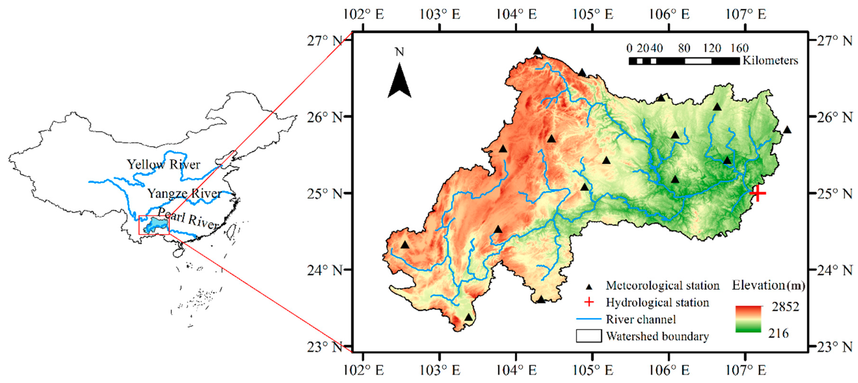
2. Study Area and Data

The North and South Panjiang basin (NSPB) (102°12′ E–107°30′ E, 23°6′ N–26°48′ N), which is one of the Pearl River sub-basins (see Figure 1), was selected as the study catchment in this study. The drainage area of the NSPB is approximately 102,199 km², which occupies about 22.5% of the Pearl River basin. The climate of this catchment is a humid monsoon climate with an annual average precipitation of 1200 mm and an annual average temperature of 16.5 °C. The flood season begins in April and ends in September, and the precipitation during this period accounts for approximately 75% of the total annual precipitation.

Table 1. Percentages of six major land use/cover types in the North and South Panjiang basin (NSPB).

Land Types	1980s	1990s	1995s	2000s	2005s	2010s
Agricultural land	22.6%	22.6%	21.7%	22.3%	22.2%	22.1%
Forest land	50.7%	50.5%	51.0%	50.3%	50.6%	50.5%
Grass land	25.5%	25.4%	25.6%	25.8%	25.6%	25.6%
Water area	0.7%	0.8%	0.7%	0.8%	0.8%	0.9%
Built-up land	0.6%	0.7%	0.9%	0.8%	0.8%	0.9%
Unused land	0.1%	0.1%	0.1%	0.1%	0.1%	0.1%

presents the percentages of six major land use/cover types from 1980 to 2010 in the NSPB. It is found that the changes in each type of land use/cover from 1980 to 2010 are not obvious, and the rate of change of all types of land cover is less than 1%, thus, it can be assumed that the land use/cover in the NSPB are almost constant from 1980 to 2010.

Tian-e hydrologic station is the outlet of the NSPB, with an average runoff of about 450 mm during 1982 to 2013, and the annual runoff data from 1982 to 2013 at this outlet were obtained from the Ministry of Water Resources of China in this study. The meteorological data obtained from 1982 to 2013 at the 15 meteorological stations, which include daily precipitation (P), average temperature (T), maximum temperature (T_max), minimum temperature (T_min), sunshine duration (S), wind speed at a height of 10 m (u) and relative humidity (RH), were provided by the China Administration of Meteorology (http://www.data.cma.cn). Additionally, the value of potential evapotranspiration (E_o) was estimated using the FAO Penman–Monteith equation [46], which can estimate E_o accurately under different climatic conditions [47,48]. The wind speed at a height of 2 m (noted as u₂) was calculated based on u using the profile relationship proposed by Allen et al. [46]. The net radiation (R_n) was calculated from S using the method recommended by Allen et al. [46], and the ground heat flux (G) was neglected because the daily and long-term average values of G are close to zero [46]. All the meteorological datasets noted above were spatially averaged by the Thiessen polygons method using ArcGIS software. To quantify the impacts of changes in vegetation coverage on E_a, the 8 km Global Inventory Modeling and Mapping Studies (GIMMS) Normalized Difference Vegetation Index (NDVI) dataset from 1982 to 2013 was derived from the Advanced Very High-Resolution Radiometer (AVHRR) sensor. Similar to climatic variables, the monthly NDVI dataset was used to represent the land surface vegetation conditions [49] of the catchment in this study. To analyze the process of land surface use/cover change in the NSPB from 1980 to 2010, a 1 km resolution land use/cover map was provided by the Resource and Environment Data Cloud Platform, Chinese Academy of Sciences (CAS) (http://www.resdc.cn/). In this study, the types of land use/cover are classified as forestland, grass land, agricultural land, built-up land, water area and unused land [21].

3. Methodology

3.1. Budyko Framework

The Budyko hypothesis indicates that terrestrial E_a is subject to the common limitations of the water supply (usually measured by P) and energy supply (usually measured by E_o) [11]. According to this hypothesis, the water supply is the limiting factor of E_a in arid catchment (E_o/P > 1), whereas energy availability is the limiting factor of E_a in humid catchments (E_o/P < 1). Based on this approach, a coupling relationship between E_a/P and E_o/P was proposed, and the general form of this relationship can be expressed as follows [11]:

$$\frac{{\mathrm{E}}_{\mathrm{a}}}{\mathrm{P}}={\left[\frac{{\mathrm{E}}_{\mathrm{o}}}{\mathrm{P}}\tanh (\frac{\mathrm{P}}{{\mathrm{E}}_{\mathrm{o}}})[1-\exp (-\frac{{\mathrm{E}}_{\mathrm{o}}}{\mathrm{P}})]\right]}^{0.5}$$

(1)

where, the units of the variables in Equation (1) are mm. Thereafter, many similar equations have been developed [35,36,37]. In this study, the three Budyko-type equations proposed by Fu [35], Zhang et al. [36] and Wang-Tang [37] (see

Table 2. The three Budyko-type equations considered in this study.

Budyko-Type Equations	Reference
$\frac{{\mathrm{E}}_{\mathrm{a}}}{\mathrm{P}}=1+\frac{{\mathrm{E}}_{\mathrm{o}}}{\mathrm{P}}-{[1+{(\frac{{\mathrm{E}}_{\mathrm{o}}}{\mathrm{P}})}^{{\mathrm{n}}^{\mathrm{F}\mathrm{u}}}]}^{1/{\mathrm{n}}^{\mathrm{F}\mathrm{u}}}$	Fu [35]
$\frac{{\mathrm{E}}_{\mathrm{a}}}{\mathrm{P}}=(1+{\mathrm{n}}^{\mathrm{Z}}\times \frac{{\mathrm{E}}_{\mathrm{o}}}{\mathrm{P}})/(1+{\mathrm{n}}^{\mathrm{Z}}\times \frac{{\mathrm{E}}_{\mathrm{o}}}{\mathrm{P}}+\frac{\mathrm{P}}{{\mathrm{E}}_{\mathrm{o}}})$	Zhang et al. [36]
$\frac{{\mathrm{E}}_{\mathrm{a}}}{\mathrm{P}}=(1+\frac{{\mathrm{E}}_{\mathrm{o}}}{\mathrm{P}}-\sqrt{{(1+\frac{{\mathrm{E}}_{\mathrm{o}}}{\mathrm{P}})}^2-4{\mathrm{n}}^{\mathrm{W}-\mathrm{T}}\times (2-{\mathrm{n}}^{\mathrm{W}-\mathrm{T}})\times \frac{{\mathrm{E}}_{\mathrm{o}}}{\mathrm{P}}})/[4{\mathrm{n}}^{\mathrm{W}-\mathrm{T}}-2{({\mathrm{n}}^{\mathrm{W}-\mathrm{T}})}^2]$	Wang-Tang [37]

) were selected to investigate the impacts of climate change and vegetation variation on E_a change. Compared with the original Budyko-type equations, which have no basin-specific parameter, the Budyko-type equations with basin-specific parameters are more flexible to account for the effects of different catchment characteristics on E_a change [50]. In this study, the basin-specific parameters in the three Budyko-type equations proposed by Fu [35], Zhang et al. [36] and Wang-Tang. [37] are expressed as n^Fu, n^Z and n^W-T, respectively.

3.2. Moving Window Method

In general, the basic water balance in closed catchments can be expressed as follows:

E_a = P − R − ΔS

(2)

where P is annual precipitation, R is annual runoff measured as streamflow and ΔS is the annual change of total water storage in the closed catchment. Because the Budyko-type equations can only be applied at the long-term average scale when ΔS is approximately zero (i.e., ΔS ≈ 0), the moving window method is applied to remove the influence of annual water storage changes in this study. Specifically, in the application of the moving window method, the width of the window size is related to the length of the variable series, and the longer window can better reduce the scatter of the variable series [13,51]; however, some specific evolution processes may be missed. According to previous studies [13,38,40], the changes of total water storage can be neglected during a long time period, and different sizes of time windows, such as 11 years and 13 years, were used in studies proposed by Jiang et al. [13] and Tian et al. [40], respectively. Here, as the P-R did not change much for time window size larger than 11 years, we selected the 11-year time window to minimize the influence of changes in ΔS series. In this study, the 11-year time window is applied to annual R, E_a, P and ΔS series, and their values in the time window centered at year t are expressed as R_t, E_at, P_t and ΔS_t, respectively. Thus, in the time window centered at year t, ΔS_t, which mainly includes changes in ground water and the plant moisture content of the catchment, can be neglected (i.e., ΔSt ≈ 0), and the water balance equation (i.e., Equation (2)) can be simplified as:

E_at = P_t − R_t.

(3)

Similar to R, E_a and P, the 11-year time window is also used for other variables, including n, T, RH, u₂, T_min, T_max, S and NDVI, the values of which, in the time window centered at year t, are expressed as n_t, T_t, RH_t, u_2t, T_mint, T_maxt, S_t and NDVI_t in the following sections.

3.3. Modeling the Parameter n_t in the Budyko-type Equations

For near-surface climate conditions, the basic meteorological factors, including P_t, T_t, T_maxt, T_mint, RH_t, u_2t and S_t, were selected as indicators to describe the variability in n_t in this study. For other factors related to land surface conditions, because the change in each type of land use/cover from 1980 to 2010 is not significant, and it can be assumed that the soil conditions and topography of a single catchment remain unchanged at the multiyear average scale, the natural variation in vegetation coverage described by NDVI in this study was selected as the only land surface variable other than climate to describe the variability in n_t in the study area. In summary, eight candidate variables, namely, P_t, T_t, T_maxt, T_mint, RH_t, u_2t, S_t and NDVI_t, were selected as the indicators of the catchment characteristics to investigate their respective relation to the variability in n_t in each Budyko-type equation.

The stepwise linear regression method was used to determine the potential relationship between the parameter n_t and the variables that were selected as the indicators of the catchment characteristics. Moreover, an empirical model is considered to explain and formulize the potential relationships, and it can be expressed as follows:

$${\mathrm{n}}_{{}_{\mathrm{t}}}^{\prime }=\mathrm{f}(\mathrm{N}\mathrm{D}\mathrm{V}{\mathrm{I}}_{\mathrm{t}},{\mathrm{P}}_{\mathrm{t}},{\mathrm{T}}_{\mathrm{t}},\mathrm{R}{\mathrm{H}}_{\mathrm{t}},{\mathrm{u}}_{2\mathrm{t}},{\mathrm{S}}_{\mathrm{t}},{\mathrm{T}}_{\min \mathrm{t}},{\mathrm{T}}_{\max \mathrm{t}}),$$

(4)

where f is a function to be determined. The parameter n_t obtained in this way is called the “modeled n_t”, which is denoted as ${\mathrm{n}}_{\mathrm{t}}^{\prime }$, and the E_at value calculated by the Budyko-type equations with ${\mathrm{n}}_{\mathrm{t}}^{\prime }$ is called “modeled E_at”, which is denoted as ${\mathrm{E}}_{\mathrm{a}\mathrm{t}}^{\prime }$. The performance of this empirical model can be evaluated by comparing the values of n_t calculated by the Budyko-type equations using the observations to the values of ${\mathrm{n}}_{\mathrm{t}}^{\prime }$. The resulting statistic, namely, the coefficient of determination (r²) and root mean squared error (RMSE), were used to evaluate the performance of this empirical formula.

3.4. Contribution Analysis

According to Wang et al. [45], assuming that each single variable is independent in the Budyko-type equations (see Table 2), the elasticity method is used to analyze the contributions of climate and vegetation changes to E_at change, and the first-order approximation of the changes in E_at can be expressed as:

$$\mathrm{d}{\mathrm{E}}_{\mathrm{a}\mathrm{t}}=\frac{\partial {\mathrm{E}}_{\mathrm{a}\mathrm{t}}}{\partial {\mathrm{P}}_{\mathrm{t}}}\mathrm{d}{\mathrm{P}}_{\mathrm{t}}+\frac{\partial {\mathrm{E}}_{\mathrm{a}\mathrm{t}}}{\partial {\mathrm{E}}_{\mathrm{o}\mathrm{t}}}\mathrm{d}{\mathrm{E}}_{\mathrm{o}\mathrm{t}}+\frac{\partial {\mathrm{E}}_{\mathrm{a}\mathrm{t}}}{\partial {\mathrm{n}}_{\mathrm{t}}}\mathrm{d}{\mathrm{n}}_{\mathrm{t}}$$

(5)

$$\begin{array}{cc}\hfill \frac{\mathrm{d}{\mathrm{E}}_{\mathrm{a}\mathrm{t}}}{{\mathrm{E}}_{\mathrm{a}\mathrm{t}}}& =\frac{\partial {\mathrm{E}}_{\mathrm{a}\mathrm{t}}}{\partial {\mathrm{P}}_{\mathrm{t}}}\frac{{\mathrm{P}}_{\mathrm{t}}}{{\mathrm{E}}_{\mathrm{a}\mathrm{t}}}\frac{\mathrm{d}{\mathrm{P}}_{\mathrm{t}}}{{\mathrm{P}}_{\mathrm{t}}}+\frac{\partial {\mathrm{E}}_{\mathrm{a}\mathrm{t}}}{\partial {\mathrm{E}}_{\mathrm{o}\mathrm{t}}}\frac{{\mathrm{E}}_{\mathrm{o}\mathrm{t}}}{{\mathrm{E}}_{\mathrm{a}\mathrm{t}}}\frac{\mathrm{d}{\mathrm{E}}_{\mathrm{o}\mathrm{t}}}{{\mathrm{E}}_{\mathrm{o}\mathrm{t}}}+\frac{\partial {\mathrm{E}}_{\mathrm{a}\mathrm{t}}}{\partial {\mathrm{n}}_{\mathrm{t}}}\frac{{\mathrm{n}}_{\mathrm{t}}}{{\mathrm{E}}_{\mathrm{a}\mathrm{t}}}\frac{\mathrm{d}{\mathrm{n}}_{\mathrm{t}}}{{\mathrm{n}}_{\mathrm{t}}}\hfill \\ & ={\epsilon }_{\mathrm{P}}\frac{\mathrm{d}{\mathrm{P}}_{\mathrm{t}}}{{\mathrm{P}}_{\mathrm{t}}}+{\epsilon }_{{\mathrm{E}}_{\mathrm{o}\mathrm{t}}}\frac{\mathrm{d}{\mathrm{E}}_{\mathrm{o}\mathrm{t}}}{{\mathrm{E}}_{\mathrm{o}\mathrm{t}}}+{\epsilon }_{{\mathrm{n}}_{\mathrm{t}}}\frac{\mathrm{d}{\mathrm{n}}_{\mathrm{t}}}{{\mathrm{n}}_{\mathrm{t}}}\hfill \end{array}$$

(6)

where ${\epsilon }_{{\mathrm{P}}_{\mathrm{t}}}, {\epsilon }_{{\mathrm{E}}_{\mathrm{o}\mathrm{t}}}$ and ${\epsilon }_{{\mathrm{n}}_{\mathrm{t}}}$ are the P_t, E_ot and n_t elasticities of E_at, and $\frac{\mathrm{d}{\mathrm{E}}_{\mathrm{o}\mathrm{t}}}{{\mathrm{E}}_{\mathrm{o}\mathrm{t}}}$ can be written as follows based on the FAO Penman–Monteith equation [45]:

$$\begin{array}{cc}\hfill \frac{\mathrm{d}{\mathrm{E}}_{\mathrm{o}\mathrm{t}}}{{\mathrm{E}}_{\mathrm{o}\mathrm{t}}}& =\frac{\partial {\mathrm{E}}_{\mathrm{o}\mathrm{t}}}{\partial {\mathrm{T}}_{\mathrm{maxt}}}\frac{1}{{\mathrm{E}}_{\mathrm{o}\mathrm{t}}}\mathrm{d}{\mathrm{T}}_{\mathrm{maxt}}+\frac{\partial {\mathrm{E}}_{\mathrm{o}\mathrm{t}}}{\partial {\mathrm{T}}_{\mathrm{mint}}}\frac{1}{{\mathrm{E}}_{\mathrm{o}\mathrm{t}}}\mathrm{d}{\mathrm{T}}_{\mathrm{mint}}+\frac{\partial {\mathrm{E}}_{\mathrm{o}\mathrm{t}}}{\partial \mathrm{R}{\mathrm{H}}_{\mathrm{t}}}\frac{\mathrm{R}{\mathrm{H}}_{\mathrm{t}}}{{\mathrm{E}}_{\mathrm{o}\mathrm{t}}}\frac{\mathrm{d}\mathrm{R}{\mathrm{H}}_{\mathrm{t}}}{\mathrm{R}{\mathrm{H}}_{\mathrm{t}}}+\frac{\partial {\mathrm{E}}_{\mathrm{o}\mathrm{t}}}{\partial {\mathrm{S}}_{\mathrm{t}}}\frac{{\mathrm{S}}_{\mathrm{t}}}{{\mathrm{E}}_{\mathrm{o}\mathrm{t}}}\frac{\mathrm{d}{\mathrm{S}}_{\mathrm{t}}}{{\mathrm{S}}_{\mathrm{t}}}+\frac{\partial {\mathrm{E}}_{\mathrm{o}\mathrm{t}}}{\partial {\mathrm{u}}_{2\mathrm{t}}}\frac{{\mathrm{u}}_{2\mathrm{t}}}{{\mathrm{E}}_{\mathrm{o}\mathrm{t}}}\frac{\mathrm{d}{\mathrm{u}}_{2\mathrm{t}}}{{\mathrm{u}}_{2\mathrm{t}}}\hfill \\ & ={\epsilon }_{{}_{{\mathrm{T}}_{\mathrm{maxt}}}}^{\prime }\mathrm{d}{\mathrm{T}}_{\mathrm{maxt}}+{\epsilon }_{{}_{{\mathrm{T}}_{\mathrm{mint}}}}^{\prime }\mathrm{d}{\mathrm{T}}_{\mathrm{mint}}+{\epsilon }_{{}_{\mathrm{R}{\mathrm{H}}_{\mathrm{t}}}}^{\prime }\frac{\mathrm{d}\mathrm{R}{\mathrm{H}}_{\mathrm{t}}}{\mathrm{R}{\mathrm{H}}_{\mathrm{t}}}+{\epsilon }_{{}_{{\mathrm{S}}_{\mathrm{t}}}}^{\prime }\frac{\mathrm{d}{\mathrm{S}}_{\mathrm{t}}}{{\mathrm{S}}_{\mathrm{t}}}+{\epsilon }_{{}_{{\mathrm{u}}_{2\mathrm{t}}}}^{\prime }\frac{\mathrm{d}{\mathrm{u}}_{2\mathrm{t}}}{{\mathrm{u}}_{2\mathrm{t}}}\hfill \end{array}$$

(7)

where ${\epsilon }_{{\mathrm{T}}_{\max \mathrm{t}}}^{\prime }$, ${\epsilon }_{{\mathrm{T}}_{\min \mathrm{t}}}^{\prime }$, ${\epsilon }_{\mathrm{R}{\mathrm{H}}_{\mathrm{t}}}^{\prime }$, ${\epsilon }_{{\mathrm{S}}_{\mathrm{t}}}^{\prime }$ and ${\epsilon }_{{\mathrm{u}}_{2\mathrm{t}}}^{\prime }$ are the T_maxt, T_mint, RH_t, S_t and u_2t elasticities of E_ot. Substituting Equation (7) into Equation (6) yields the following expression:

$$\begin{array}{ll}\frac{\mathrm{d}{\mathrm{E}}_{\mathrm{a}\mathrm{t}}}{{\mathrm{E}}_{\mathrm{a}\mathrm{t}}}& ={\epsilon }_{\mathrm{P}}\frac{\mathrm{d}{\mathrm{P}}_{\mathrm{t}}}{{\mathrm{P}}_{\mathrm{t}}}+{\epsilon }_{{\mathrm{E}}_{\mathrm{o}\mathrm{t}}}{\epsilon }_{{}_{{\mathrm{T}}_{\mathrm{maxt}}}}^{\prime }\mathrm{d}{\mathrm{T}}_{\mathrm{maxt}}+{\epsilon }_{{\mathrm{E}}_{\mathrm{o}\mathrm{t}}}{\epsilon }_{{}_{{\mathrm{T}}_{\mathrm{mint}}}}^{\prime }\mathrm{d}{\mathrm{T}}_{\mathrm{mint}}+{\epsilon }_{{\mathrm{E}}_{\mathrm{o}\mathrm{t}}}{\epsilon }_{{}_{\mathrm{R}{\mathrm{H}}_{\mathrm{t}}}}^{\prime }\frac{\mathrm{d}\mathrm{R}{\mathrm{H}}_{\mathrm{t}}}{\mathrm{R}{\mathrm{H}}_{\mathrm{t}}}+{\epsilon }_{{\mathrm{E}}_{\mathrm{o}\mathrm{t}}}{\epsilon }_{{}_{{\mathrm{S}}_{\mathrm{t}}}}^{\prime }\frac{\mathrm{d}{\mathrm{S}}_{\mathrm{t}}}{{\mathrm{S}}_{\mathrm{t}}}+{\epsilon }_{{\mathrm{E}}_{\mathrm{o}\mathrm{t}}}{\epsilon }_{{}_{{\mathrm{u}}_{2\mathrm{t}}}}^{\prime }\frac{\mathrm{d}{\mathrm{u}}_{2\mathrm{t}}}{{\mathrm{u}}_{2\mathrm{t}}}+{\epsilon }_{{\mathrm{n}}_{\mathrm{t}}}\frac{\mathrm{d}{\mathrm{n}}_{\mathrm{t}}}{{\mathrm{n}}_{\mathrm{t}}}\\ & ={\epsilon }_{\mathrm{P}}\frac{\mathrm{d}{\mathrm{P}}_{\mathrm{t}}}{{\mathrm{P}}_{\mathrm{t}}}+{\epsilon }_{{\mathrm{T}}_{\mathrm{maxt}}}\mathrm{d}{\mathrm{T}}_{\mathrm{maxt}}+{\epsilon }_{{\mathrm{T}}_{\mathrm{mint}}}\mathrm{d}{\mathrm{T}}_{\mathrm{mint}}+{\epsilon }_{\mathrm{R}{\mathrm{H}}_{\mathrm{t}}}\frac{\mathrm{d}\mathrm{R}{\mathrm{H}}_{\mathrm{t}}}{\mathrm{R}{\mathrm{H}}_{\mathrm{t}}}+{\epsilon }_{{\mathrm{S}}_{\mathrm{t}}}\frac{\mathrm{d}{\mathrm{S}}_{\mathrm{t}}}{{\mathrm{S}}_{\mathrm{t}}}+{\epsilon }_{{\mathrm{u}}_{2\mathrm{t}}}\frac{\mathrm{d}{\mathrm{u}}_{2\mathrm{t}}}{{\mathrm{u}}_{2\mathrm{t}}}+{\epsilon }_{{\mathrm{n}}_{\mathrm{t}}}\frac{\mathrm{d}{\mathrm{n}}_{\mathrm{t}}}{{\mathrm{n}}_{\mathrm{t}}}\end{array}$$

(8)

where ${\epsilon }_{{\mathrm{T}}_{\max \mathrm{t}}}^{}$, ${\epsilon }_{{\mathrm{T}}_{\min \mathrm{t}}}^{}$, ${\epsilon }_{\mathrm{R}{\mathrm{H}}_{\mathrm{t}}}^{}$, ${\epsilon }_{{\mathrm{S}}_{\mathrm{t}}}^{}$ and ${\epsilon }_{{\mathrm{u}}_{2\mathrm{t}}}^{}$ are the T_maxt, T_mint, RH_t, S_t and u_2t elasticities of E_at. Thus, the changes in E_at induced by variations in all the independent variables can be estimated as:

$$\begin{array}{ccc}\hfill \Delta {\mathrm{E}}_{\mathrm{a}\mathrm{t}}& \hfill =& \Delta {\mathrm{E}}_{\mathrm{a}\mathrm{t}-{\mathrm{P}}_{\mathrm{t}}}+\Delta {\mathrm{E}}_{\mathrm{a}\mathrm{t}-{\mathrm{T}}_{\max \mathrm{t}}}+\Delta {\mathrm{E}}_{\mathrm{a}\mathrm{t}-{\mathrm{T}}_{\min \mathrm{t}}}+\Delta {\mathrm{E}}_{\mathrm{a}\mathrm{t}-\mathrm{R}{\mathrm{H}}_{\mathrm{t}}}+\Delta {\mathrm{E}}_{\mathrm{a}\mathrm{t}-{\mathrm{S}}_{\mathrm{t}}}+\Delta {\mathrm{E}}_{\mathrm{a}\mathrm{t}-{\mathrm{u}}_{2\mathrm{t}}}+\Delta {\mathrm{E}}_{\mathrm{a}\mathrm{t}-{\mathrm{n}}_{\mathrm{t}}}\hfill \\ & \hfill =& {\epsilon }_{\mathrm{P}}\frac{{\mathrm{E}}_{\mathrm{a}\mathrm{t}}}{{\mathrm{P}}_{\mathrm{t}}}\Delta {\mathrm{P}}_{\mathrm{t}}+{\epsilon }_{{\mathrm{T}}_{\mathrm{maxt}}}{\mathrm{E}}_{\mathrm{a}\mathrm{t}}\Delta {\mathrm{T}}_{\mathrm{maxt}}+{\epsilon }_{{\mathrm{T}}_{\mathrm{mint}}}{\mathrm{E}}_{\mathrm{a}\mathrm{t}}\Delta {\mathrm{T}}_{\mathrm{mint}}+{\epsilon }_{\mathrm{R}{\mathrm{H}}_{\mathrm{t}}}\frac{{\mathrm{E}}_{\mathrm{a}\mathrm{t}}}{\mathrm{R}{\mathrm{H}}_{\mathrm{t}}}\Delta \mathrm{R}{\mathrm{H}}_{\mathrm{t}}\hfill \\ & & +{\epsilon }_{{\mathrm{S}}_{\mathrm{t}}}\frac{{\mathrm{E}}_{\mathrm{a}\mathrm{t}}}{{\mathrm{S}}_{\mathrm{t}}}\Delta {\mathrm{S}}_{\mathrm{t}}+{\epsilon }_{{\mathrm{u}}_{2\mathrm{t}}}\frac{{\mathrm{E}}_{\mathrm{a}\mathrm{t}}}{{\mathrm{u}}_{2\mathrm{t}}}\Delta {\mathrm{u}}_{2\mathrm{t}}+{\epsilon }_{{\mathrm{n}}_{\mathrm{t}}}\frac{{\mathrm{E}}_{\mathrm{a}\mathrm{t}}}{{\mathrm{n}}_{\mathrm{t}}}\Delta {\mathrm{n}}_{\mathrm{t}}\hfill \end{array}$$

(9)

and the relative contributions of single variable to E_at change can be calculated as follows:

$${\eta }_{\mathrm{v}\mathrm{i}}=\frac{\Delta {\mathrm{E}}_{\mathrm{a}\mathrm{t}-\mathrm{v}\mathrm{i}}}{\Delta {\mathrm{E}}_{\mathrm{a}\mathrm{t}}}\times 100\%$$

(10)

where vi is a variable (such as P_t, T_maxt, T_mint, RH_t, u_2t, S_t), and ${\eta }_{\mathrm{v}\mathrm{i}}$ is the relative contribution of changes in vi to E_at changes.

4. Results and Discussion

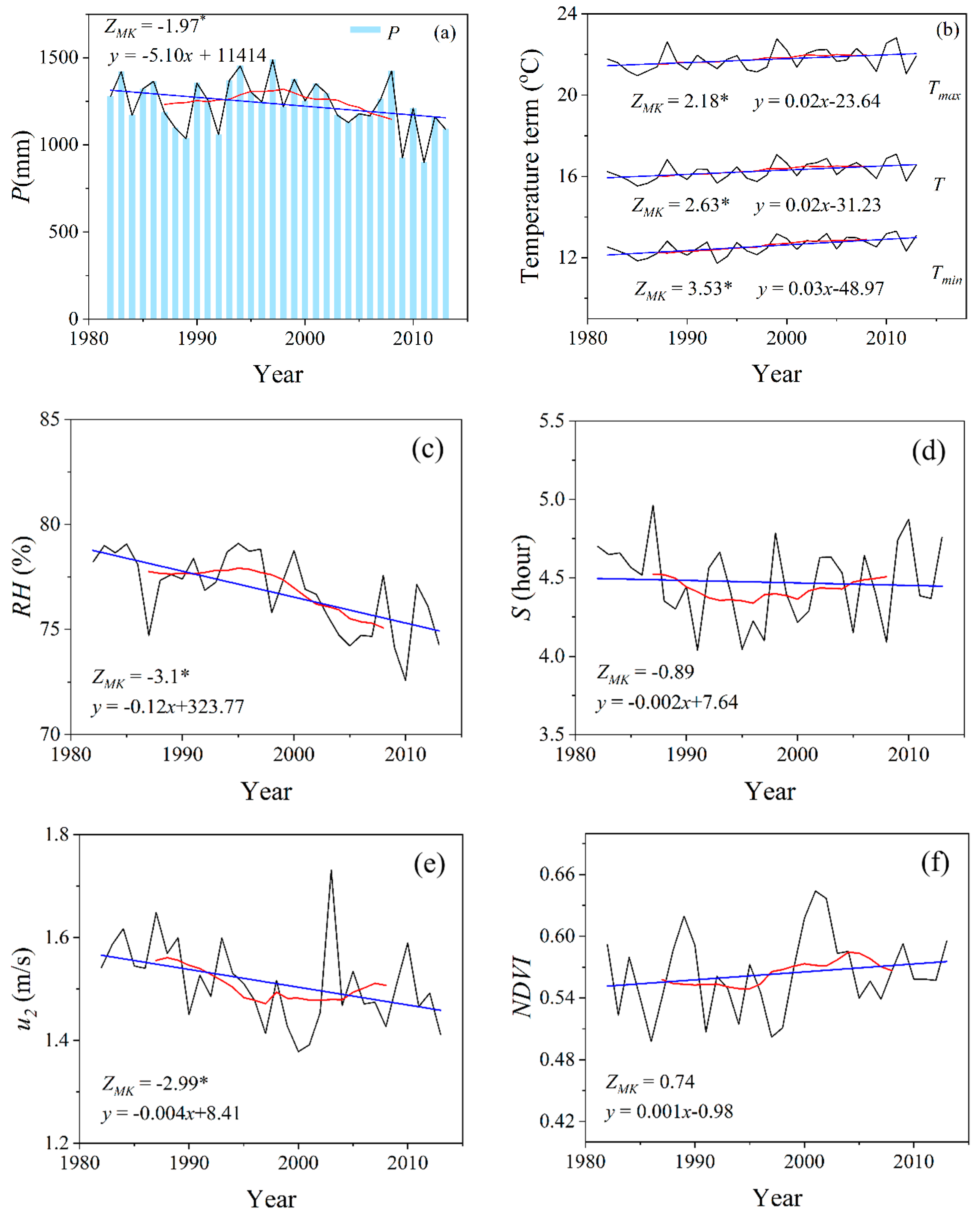
4.1. Temporal Variations in Climatic Variables and the NDVI

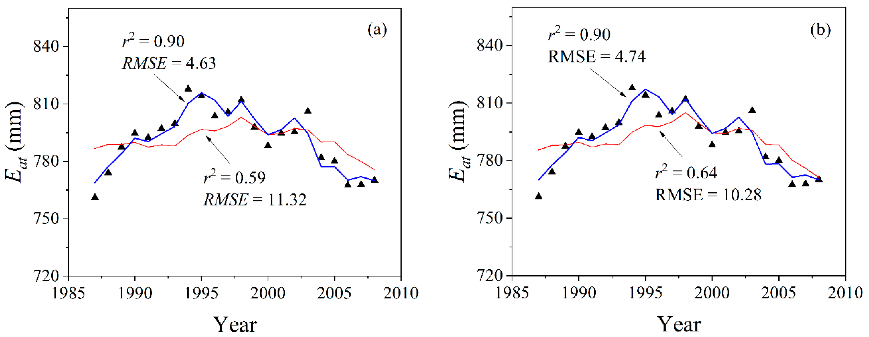
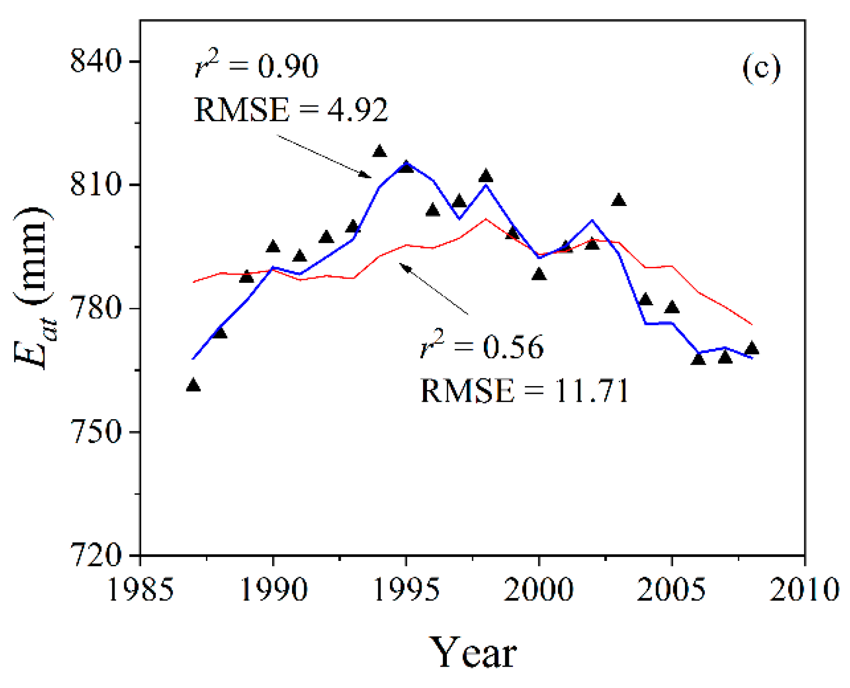
To investigate the temporal variations in meteorological factors and the NDVI from 1982 to 2013 in the NSPB, the nonparametric trend-free pre-whitening Mann–Kendall test developed by Mann [52], Kendall [53] and Yue et al. [54,55] was used in this section. As shown in Figure 2, significant warming can be observed in the study area, as the annual T, T_max and T_min values displayed an evident increasing trend at the 0.05 significance level, which is consistent with the general trends of the global warming [56] and warming in China [57]. Wind speed has significantly decreased, which supports the results given by McVicar et al. [58]. Similar to the wind speed, annual P and RH also exhibit significant decreasing trends. In addition, S presents a slight decreasing trend, and the NDVI in the study area displays a slight increasing trend (p-value > 0.05).

4.2. Modeling $n_t^{\prime }$

A stepwise regression method was used to establish the potential relationship between the parameter n_t and the eight candidate variables (discussed in Section 3.3) selected as the indicators of the catchment characteristics. The results of stepwise regression show that the parameter n_t simulated with four candidate variables, including S_t, NDVI_t, T_maxt and P_t, yields a satisfactory determination coefficient, r², between ${\mathrm{n}}_{\mathrm{t}}^{\prime }$ and n_t calculated by the Budyko-type equations using the observations. As shown in

Table 3. Stepwise regression results between n_t and the surface candidate variables in the NSPB.

Variable	Step	r2
		Fu	Zhang	Wang-Tang
St	1	0.62	0.57	0.65
St, NDVIt	2	0.71	0.64	0.72
St, NDVIt, Tmaxt	3	0.79	0.76	0.79
St, NDVIt, Tmaxt, Pt	4	0.82	0.78	0.84
St, NDVIt, Tamxt, Pt, RHt, u2t, Tt, Tmint	5	0.83	0.79	0.84

, the first candidate variable entered into the stepwise regression equation was S_t, which resulted in r² values greater than 0.5 among the three parameters, ${\mathrm{n}}_{\mathrm{t}}^{\prime }$. The other three selected candidate variables, namely, NDVI_t, T_maxt and P_t, increased r² by more than 0.02. The use of remaining candidate variables (such as RH_t, u_2t, T_t and T_mint) did not effectively increase the r² value. Therefore, S_t, NDVI_t, T_maxt and P_t were identified as the decision variables and used to predict the parameter n_t in this study, and the final fitted model of ${\mathrm{n}}_{\mathrm{t}}^{\prime }$ in each Budyko-type equation was obtained as:

$${\mathrm{n}}_{\mathrm{t}}^{\mathrm{F}\mathrm{u}\prime }=-2.23\ln {\mathrm{S}}_{\mathrm{t}}-4.34\ln \mathrm{N}\mathrm{D}\mathrm{V}{\mathrm{I}}_{\mathrm{t}}+9.77\ln {\mathrm{T}}_{\max \mathrm{t}}+0.82\ln {\mathrm{P}}_{\mathrm{t}}-27.55$$

(11a)

$${\mathrm{n}}_{\mathrm{t}}^{\mathrm{Z}\prime }=-2.51\ln {\mathrm{S}}_{\mathrm{t}}-4.87\ln \mathrm{N}\mathrm{D}\mathrm{V}{\mathrm{I}}_{\mathrm{t}}+11.24\ln {\mathrm{T}}_{\max \mathrm{t}}+0.58\ln {\mathrm{P}}_{\mathrm{t}}-33.00$$

(11b)

$${\mathrm{n}}_{\mathrm{t}}^{\mathrm{W}-\mathrm{T}\prime }=-0.56\ln {\mathrm{S}}_{\mathrm{t}}-1.05\ln \mathrm{N}\mathrm{D}\mathrm{V}{\mathrm{I}}_{\mathrm{t}}+2.42\ln {\mathrm{T}}_{\max \mathrm{t}}+0.23\ln {\mathrm{P}}_{\mathrm{t}}-6.90$$

(11c)

Figure 3 compares the values of ${\mathrm{n}}_{\mathrm{t}}^{\prime }$ estimated using Equations (11a)–(11c), with the n_t values estimated based on observations using each Budyko-type equation. The modeled ${\mathrm{n}}_{\mathrm{t}}^{\prime }$ values are closely correlated with n_t, and the r² values are all greater than 0.78, suggesting that the relationships in these three empirical equations can accurately encompass the impacts of climatic factors and NDVI_t on n_t. From these empirical formulas of modeled ${\mathrm{n}}_{\mathrm{t}}^{\prime }$, it can be found that climate change affects E_at by simultaneously influencing the meteorological inputs (such as P_t and E_ot) and the basin-specific parameter n_t, while the NDVI_t change affects E_at implemented by the alteration of the parameter n_t in the NSPB from 1982 to 2013. Moreover, the sign of each coefficient in Equations (11a)–(11c) can reflect the relationship between the changes in variables and ${\mathrm{n}}_{\mathrm{t}}^{\prime }$ change. Generally, a positive (or negative) coefficient means that ${\mathrm{n}}_{\mathrm{t}}^{\prime }$ will increase (or decrease) as the value of the variable increases. Thus, we can shortly draw from Equations (11a)–(11c) that ${\mathrm{n}}_{\mathrm{t}}^{\prime }$ decreases as S_t and NDVI_t increase, and ${\mathrm{n}}_{\mathrm{t}}^{\prime }$ increases as P_t and T_maxt increase. However, the sign of each coefficient in Equations (11a)–(11c) cannot reflect the contribution of each related change to ${\mathrm{n}}_{\mathrm{t}}^{\prime }$ change, which will be further analyzed in the next section. Additionally, it is worth noting that the coefficient of each variable in Equations (11a)–(11c) is basin-specific, it should recalibrate in other catchments or regions which with different climate and vegetation conditions.

Additionally, the empirical formula for n_t is used together with the Budyko-type equations to calibrate the E_at estimation in the NSPB. In this study, two methods of E_at estimation were considered for comparison: (i) using the time-varying ${\mathrm{n}}_{\mathrm{t}}^{\prime }$ calculated by Equations (11a)–(11c) with time-varying variables and (ii) using the constant parameter n_t calculated with the long-term average variables. Figure 4 shows the comparison between the values of E_at obtained from the water balance equation (i.e., Equation (3)) and these two cases. The r² values with a constant n_t vary from 0.55 to 0.61, and the r² values with a time-varying ${\mathrm{n}}_{\mathrm{t}}^{\prime }$ are all larger than 0.90. This result indicates that the performance of each Budyko-type equation with a time-varying ${\mathrm{n}}_{\mathrm{t}}^{\prime }$ is better than that for a constant n_t, which is consistent with the findings of Yang et al. [21], Jiang et al. [13] and Tian et al. [40]. Therefore, compared with the temporally constant parameter n which was used in most previous studies [25,32,33,44,59], the time-varying parameter n improves the accuracy of E_a simulation based on the Budyko-type equations and specifically describes the evolution process of E_a in the NSPB.

4.3. Quantitative Contributions to E_at Variation

Based on the analysis in Section 4.2, both climate change and vegetation variations will affect E_at variations in the NSPB. Moreover, combining the empirical equation for n_t estimation (i.e., Equations (11a)–(11c)) and the FAO Penman–Monteith equation, which was used to estimate E_o, the Budyko-type equations used in this study can be written as ${\mathrm{E}}_{\mathrm{a}\mathrm{t}}=\mathrm{f}({\mathrm{P}}_{\mathrm{t}},{\mathrm{T}}_{\max \mathrm{t}},{\mathrm{T}}_{\min \mathrm{t}},{\mathrm{S}}_{\mathrm{t}},\mathrm{R}{\mathrm{H}}_{\mathrm{t}},{\mathrm{u}}_{2\mathrm{t}},\mathrm{N}\mathrm{D}\mathrm{V}{\mathrm{I}}_{\mathrm{t}})$. Therefore, based on Equations (8) and (9), the change in E_at ($\Delta {\mathrm{E}}_{\mathrm{a}\mathrm{t}}$) can be further expressed as:

$$\begin{array}{ccc}\hfill \Delta {\mathrm{E}}_{\mathrm{a}\mathrm{t}}& =& \Delta {\mathrm{E}}_{\mathrm{a}\mathrm{t}-{\mathrm{P}}_{\mathrm{t}}}{}^{}+\Delta {\mathrm{E}}_{\mathrm{a}\mathrm{t}-{\mathrm{T}}_{\max \mathrm{t}}}{}^{}+\Delta {\mathrm{E}}_{\mathrm{a}\mathrm{t}-{\mathrm{T}}_{\min \mathrm{t}}}{}^{}+\Delta {\mathrm{E}}_{\mathrm{a}\mathrm{t}-{\mathrm{S}}_{\mathrm{t}}}{}^{}+\Delta {\mathrm{E}}_{\mathrm{a}\mathrm{t}-\mathrm{R}{\mathrm{H}}_{\mathrm{t}}}{}^{}+\Delta {\mathrm{E}}_{\mathrm{a}\mathrm{t}-{\mathrm{u}}_{2\mathrm{t}}}{}^{}+\Delta {\mathrm{E}}_{\mathrm{a}\mathrm{t}-\mathrm{N}\mathrm{D}\mathrm{V}{\mathrm{I}}_{\mathrm{t}}}{}^{}\hfill \\ & =& {\epsilon }_{{\mathrm{P}}_{\mathrm{t}}}\frac{{\mathrm{E}}_{\mathrm{a}\mathrm{t}}}{{\mathrm{P}}_{\mathrm{t}}}\Delta {\mathrm{P}}_{\mathrm{t}}+{\epsilon }_{{\mathrm{T}}_{\max \mathrm{t}}}{\mathrm{E}}_{\mathrm{a}\mathrm{t}}\Delta {\mathrm{T}}_{\max \mathrm{t}}+{\epsilon }_{{\mathrm{T}}_{\min \mathrm{t}}}{\mathrm{E}}_{\mathrm{a}\mathrm{t}}\Delta {\mathrm{T}}_{\min \mathrm{t}}+{\epsilon }_{\mathrm{S}}\frac{{\mathrm{E}}_{\mathrm{a}\mathrm{t}}}{{\mathrm{S}}_{\mathrm{t}}}\Delta {\mathrm{S}}_{\mathrm{t}}+{\epsilon }_{\mathrm{R}{\mathrm{H}}_{\mathrm{t}}}\frac{{\mathrm{E}}_{\mathrm{a}\mathrm{t}}}{\mathrm{R}{\mathrm{H}}_{\mathrm{t}}}\Delta \mathrm{R}{\mathrm{H}}_{\mathrm{t}}+{\epsilon }_{{\mathrm{u}}_{2\mathrm{t}}}\frac{{\mathrm{E}}_{\mathrm{a}\mathrm{t}}}{{\mathrm{u}}_{2\mathrm{t}}}\Delta {\mathrm{u}}_{2\mathrm{t}}\hfill \\ & & +{\epsilon }_{\mathrm{N}\mathrm{D}\mathrm{V}{\mathrm{I}}_{\mathrm{t}}}\frac{{\mathrm{E}}_{\mathrm{a}}}{\mathrm{N}\mathrm{D}\mathrm{V}{\mathrm{I}}_{\mathrm{t}}}\Delta \mathrm{N}\mathrm{D}\mathrm{V}{\mathrm{I}}_{\mathrm{t}}\hfill \end{array}$$

(12)

where $\Delta {\mathrm{E}}_{\mathrm{a}\mathrm{t}-{\mathrm{P}}_{\mathrm{t}}}$, $\Delta {\mathrm{E}}_{\mathrm{a}\mathrm{t}-{\mathrm{T}}_{\max \mathrm{t}}}$, $\Delta {\mathrm{E}}_{\mathrm{a}\mathrm{t}-{\mathrm{T}}_{\min \mathrm{t}}}$, $\Delta {\mathrm{E}}_{\mathrm{a}\mathrm{t}-{\mathrm{S}}_{\mathrm{t}}}$, $\Delta {\mathrm{E}}_{\mathrm{a}\mathrm{t}-\mathrm{R}{\mathrm{H}}_{\mathrm{t}}}$, $\Delta {\mathrm{E}}_{\mathrm{a}\mathrm{t}-{\mathrm{u}}_{2\mathrm{t}}}$ and $\Delta {\mathrm{E}}_{\mathrm{a}\mathrm{t}-\mathrm{N}\mathrm{D}\mathrm{V}{\mathrm{I}}_{\mathrm{t}}}$ represent the changes in E_at due to changes in P_t, T_maxt, T_mint, S_t, RH_t, u_2t and NDVI_t, respectively. As in Equation (9), the elasticity of E_at to climatic factors and NDVI_t can be estimated as ${\epsilon }_{{\mathrm{P}}_{\mathrm{t}}}=\frac{\partial \mathrm{f}}{\partial {\mathrm{P}}_{\mathrm{t}}}\frac{{\mathrm{P}}_{\mathrm{t}}}{{\mathrm{E}}_{\mathrm{a}\mathrm{t}}}$,${\epsilon }_{{\mathrm{T}}_{\max \mathrm{t}}}=\frac{\partial \mathrm{f}}{\partial {\mathrm{T}}_{\max \mathrm{t}}{}_{\mathrm{t}}}\frac{1}{{\mathrm{E}}_{\mathrm{a}\mathrm{t}}}$, ${\epsilon }_{{\mathrm{T}}_{\min \mathrm{t}}}=\frac{\partial \mathrm{f}}{\partial {\mathrm{T}}_{\min \mathrm{t}}}\frac{1}{{\mathrm{E}}_{\mathrm{a}\mathrm{t}}}$,${\epsilon }_{{\mathrm{S}}_{\mathrm{t}}}=\frac{\partial \mathrm{f}}{\partial {\mathrm{S}}_{\mathrm{t}}}\frac{{\mathrm{S}}_{\mathrm{t}}}{{\mathrm{E}}_{\mathrm{a}\mathrm{t}}}$,${\epsilon }_{\mathrm{R}{\mathrm{H}}_{\mathrm{t}}}=\frac{\partial \mathrm{f}}{\partial \mathrm{R}{\mathrm{H}}_{\mathrm{t}}}\frac{\mathrm{R}{\mathrm{H}}_{\mathrm{t}}}{{\mathrm{E}}_{\mathrm{a}\mathrm{t}}}$,${\epsilon }_{{\mathrm{u}}_{2\mathrm{t}}}=\frac{\partial \mathrm{f}}{\partial {\mathrm{u}}_{2\mathrm{t}}}\frac{{\mathrm{u}}_{2\mathrm{t}}}{{\mathrm{E}}_{\mathrm{a}\mathrm{t}}}$ and ${\epsilon }_{\mathrm{N}\mathrm{D}\mathrm{V}{\mathrm{I}}_{\mathrm{t}}}=\frac{\partial \mathrm{f}}{\partial \mathrm{N}\mathrm{D}\mathrm{V}{\mathrm{I}}_{\mathrm{t}}}\frac{\mathrm{N}\mathrm{D}\mathrm{V}{\mathrm{I}}_{\mathrm{t}}}{{\mathrm{E}}_{\mathrm{a}\mathrm{t}}}$. In this section, the period of 1982–1992 is treated as the benchmark (pre-change period), and the following time widows are individually treated as post-change periods.

Equation (12) is used to analyze the contribution of climate change and vegetation variations to E_at change ($\Delta {\mathrm{E}}_{\mathrm{a}\mathrm{t}}$) in each post-change period, which is estimated by subtracting the value of E_at in the first time window (the period of 1982–1992). The results based on the equation proposed by Zhang et al. [36] were selected for analysis in this section, because the results of all three Budyko-type equations are very similar. First, the elasticity of E_at to all variables in each time window is shown in

Table 4. Elasticity of E_at to variables in different time windows based on the equation proposed by Zhang et al. [36].

Time Window	Elasticity of Eat to Variables
	${\mathit{\epsilon }}_{{\mathbf{P}}_{\mathbf{t}}}$	${\mathit{\epsilon }}_{{\mathbf{T}}_{\mathbf{max}\mathbf{t}}}$	${\mathit{\epsilon }}_{{\mathbf{T}}_{\mathbf{min}\mathbf{t}}}$	${\mathit{\epsilon }}_{\mathbf{R}{\mathbf{H}}_{\mathbf{t}}}$	${\mathit{\epsilon }}_{{\mathbf{S}}_{\mathbf{t}}}$	${\mathit{\epsilon }}_{{\mathbf{u}}_{\mathbf{2}\mathbf{t}}}$	${\mathit{\epsilon }}_{\mathbf{N}\mathbf{D}\mathbf{V}{\mathbf{I}}_{\mathbf{t}}}$
1982–1992	0.56	0.09	0.006	−0.36	−0.22	0.03	−0.75
1983–1993	0.55	0.09	0.006	−0.36	−0.21	0.03	−0.73
1984–1994	0.55	0.08	0.006	−0.35	−0.19	0.03	−0.70
1985–1995	0.54	0.08	0.006	−0.35	−0.18	0.03	−0.68
1986–1996	0.54	0.08	0.006	−0.35	−0.18	0.03	−0.67
1987–1997	0.54	0.08	0.006	−0.35	−0.18	0.03	−0.67
1988–1998	0.54	0.08	0.006	−0.35	−0.17	0.03	−0.65
1989–1999	0.53	0.08	0.006	−0.35	−0.16	0.03	−0.64
1990–2000	0.53	0.08	0.006	−0.35	−0.16	0.03	−0.64
1991–2001	0.53	0.08	0.006	−0.36	−0.17	0.03	−0.66
1992–2002	0.53	0.08	0.006	−0.35	−0.18	0.03	−0.69
1993–2003	0.53	0.08	0.006	−0.36	−0.18	0.04	−0.68
1994–2004	0.54	0.08	0.006	−0.35	−0.19	0.04	−0.70
1995–2005	0.55	0.08	0.006	−0.34	−0.19	0.04	−0.70
1996–2006	0.55	0.08	0.006	−0.33	−0.19	0.04	−0.68
1997–2007	0.56	0.08	0.006	−0.33	−0.18	0.04	−0.67
1998–2008	0.55	0.08	0.005	−0.32	−0.19	0.04	−0.68
1999–2009	0.56	0.08	0.005	−0.32	−0.21	0.04	−0.72
2000–2010	0.57	0.08	0.005	−0.31	−0.21	0.04	−0.71
2001–2011	0.58	0.08	0.005	−0.31	−0.20	0.04	−0.70
2002–2012	0.59	0.08	0.005	−0.30	−0.19	0.04	−0.67
2003–2013	0.59	0.08	0.005	−0.29	−0.18	0.04	−0.64

. Notably, the elasticity of E_at to P_t, T_maxt, T_mint and u_2t is positive, which indicates that an increase (decrease) in these variables will increase (decrease) E_at in the study area. To the contrary, the elasticity of E_at to RH_t, S_t and NDVI_t is negative, which indicates that an increase (decrease) in these variables will decrease (increase) E_at. In addition, the magnitude of the elasticity also reflects the sensitivity level of E_at to these variables, the greater the absolute value of the elasticity is, the more impact the variable has on E_at. Thus, E_at is more sensitive to NDVI_t and P_t than other variables in the NSPB, while the absolute values of elasticity are higher for NDVI_t and P_t than for other variables. Then, considering the changes of each variable in each time window relative to the values in the pre-change period (1982–1992) and the elasticity of E_at to all variables, the contributions of P_t, T_maxt, T_mint, RH_t, S_t, u_2t and NDVI_t to $\Delta {\mathrm{E}}_{\mathrm{a}\mathrm{t}}$ can be obtained, and the results are shown in

Table 5. The contributions of variables in different time windows based on the equation proposed by Zhang et al. [36] and $\Delta {\mathrm{E}}_{\mathrm{a} \mathrm{t}}$ for each time window was estimated by Equation (12).

Time Window	$\mathbf{\Delta }{\mathbf{E}}_{\mathbf{a}\mathbf{t}}\left(\mathbf{mm}\right)$	$\mathbf{Contribution}\mathbf{Rate}\mathbf{of}\mathbf{Variables}\mathbf{to}\mathbf{\Delta }{\mathbf{E}}_{\mathbf{a} \mathbf{t}}(\%)$
		${\mathit{\eta }}_{{\mathbf{P}}_{\mathbf{t}}}$	${\mathit{\eta }}_{{\mathbf{T}}_{\mathbf{max}\mathbf{t}}}$	${\mathit{\eta }}_{{\mathbf{T}}_{\mathbf{min}\mathbf{t}}}$	${\mathit{\eta }}_{\mathbf{R}{\mathbf{H}}_{\mathbf{t}}}$	${\mathit{\eta }}_{{\mathbf{S}}_{\mathbf{t}}}$	${\mathit{\eta }}_{{\mathbf{u}}_{\mathbf{2}\mathbf{t}}}$	${\mathit{\eta }}_{\mathbf{C}}$	${\mathit{\eta }}_{\mathbf{V}}={\mathit{\eta }}_{\mathbf{N}\mathbf{D}\mathbf{V}{\mathbf{I}}_{\mathbf{t}}}$
1982–1992	0	0	0	0	0	0	0	0	0
1983–1993	12.83	34.97	11.90	−1.46	3.82	1.44	1.05	51.71	48.29
1984–1994	26.34	25.17	35.30	0.74	2.70	5.70	0.01	69.62	30.38
1985–1995	33.54	34.11	30.23	1.36	1.17	11.47	−0.71	77.63	22.37
1986–1996	31.30	26.57	31.57	1.85	1.81	17.35	−1.28	77.88	22.12
1987–1997	35.97	36.89	26.22	1.98	0.57	19.26	−1.87	83.04	16.96
1988–1998	38.61	35.25	24.96	2.21	−0.70	17.67	−2.32	77.07	22.93
1989–1999	56.70	43.88	25.59	2.16	−0.46	11.46	−2.20	80.43	19.57
1990–2000	52.97	50.34	23.71	2.15	−1.17	10.29	−2.68	82.63	17.37
1991–2001	42.48	53.41	26.77	2.66	−0.90	12.37	−3.11	91.19	8.81
1992–2002	44.65	65.39	42.84	3.17	0.40	11.29	−4.06	119.03	−19.03
1993–2003	50.80	61.11	47.32	3.99	1.21	8.74	−2.53	119.86	−19.86
1994–2004	36.74	58.43	57.25	5.28	3.64	12.30	−3.80	133.1	−33.10
1995–2005	26.95	49.46	70.47	7.16	9.64	19.38	−5.11	151.01	−51.01
1996–2006	33.51	32.76	82.19	7.23	12.91	11.13	−4.99	141.23	−41.23
1997–2007	34.21	29.32	79.32	6.75	14.22	7.70	−4.39	132.92	−32.92
1998–2008	44.92	30.14	98.67	8.61	19.26	10.48	−5.52	161.64	−61.64
1999–2009	20.77	−3.94	224.44	19.62	47.74	27.45	−12.82	302.48	−202.48
2000–2010	18.91	−52.85	275.52	22.48	64.00	15.93	−11.57	313.52	−213.52
2001–2011	6.34	−187.26	413.65	35.37	108.67	17.64	−16.13	371.94	−271.94
2002–2012	6.78	−352.40	470.48	43.69	133.65	15.94	−15.96	295.39	−195.39
2003–2013	8.99	−317.01	380.31	36.46	114.56	7.11	−14.01	207.42	−107.42

. From this table, it is found that the changes in P_t, T_maxt and NDVI_t contributed most to $\Delta {\mathrm{E}}_{\mathrm{a}\mathrm{t}}$, while the absolute values of these contributions are relatively high compared with those of other factors. The changes in u_2t and T_mint have limited impacts on $\Delta {\mathrm{E}}_{\mathrm{a}\mathrm{t}}$ because the corresponding absolute values of the contributions are very low. Moreover, T_maxt and T_mint positively contribute to the E_at increase in all time windows, because the values of elasticity and changes are all positive during the study period. S_t makes a positive contribution to the E_at increase because the values of elasticity and changes are all negative during the study period. Because the elasticity of E_at to P_t is positive in all time windows and P_t increased in time windows from 1983–1993 to 1998–2008 but decreased during the time windows from 1999–2009 to 2003–2013, P_t contributed positively to the E_at increase during the time windows from 1983–1993 to 1998–2008 but contributed negatively during the time windows from 1999–2009 to 2003–2013. Similarly, the changes in NDVI_t, RH_t and u_2t all showed both positive and negative contributions to the E_at increase. Additionally, the contribution of climate change (${\eta }_{\mathrm{C}}$) to $\Delta {\mathrm{E}}_{\mathrm{a}\mathrm{t}}$ can be obtained by summing all the contribution rates of related climatic variables (i.e.,${\eta }_{\mathrm{C}}={\eta }_{{\mathrm{P}}_{\mathrm{t}}}+{\eta }_{{\mathrm{T}}_{\max \mathrm{t}}}+{\eta }_{{\mathrm{T}}_{\min \mathrm{t}}}+{\eta }_{\mathrm{R}{\mathrm{H}}_{\mathrm{t}}}+{\eta }_{{\mathrm{S}}_{\mathrm{t}}}+{\eta }_{{\mathrm{u}}_{2\mathrm{t}}}$), while the contribution of vegetation change (${\eta }_{\mathrm{V}}$) to $\Delta {\mathrm{E}}_{\mathrm{a}\mathrm{t}}$ is obtained by the contribution rate of NDVI (i.e.,${\eta }_{\mathrm{V}}={\eta }_{\mathrm{N}\mathrm{D}\mathrm{V}{\mathrm{I}}_{\mathrm{t}}}$). Overall, climate change contributed more to $\Delta {\mathrm{E}}_{\mathrm{a}\mathrm{t}}$ than vegetation change, and the change in vegetation contributed positively during the time windows from 1982–1992 to 1992–2002 but negatively during the time windows from 1993–2003 to 2003–2013.

The contributions to E_at variation obtained in this study matched those estimated in previous studies in China, such as by Yang and Yang [43] and Wang et al. [45], who demonstrated that precipitation changes were mainly responsible for the variations of evapotranspiration and runoff among the basic climatic variables. Additionally, for the temperature index, the elasticity of E_at to T_maxt is significantly greater than that to T_mint in the NSPB, mainly because T_max was used to calculate several important terms in the E_o and E_a estimation process, such as net radiation at the crop surface (R_n), the saturation vapor pressure (e_s), and the slops of the saturation vapor pressure versus air temperature curve (Δ). Additionally, the values of T_max are always greater than T_mint at any time of the day and in any season [60]. Furthermore, the variation in the NDVI, which was selected as the indicator of vegetation conditions, has a large influence on the change in E_a. In fact, many studies have explored how vegetation coverage influences basin-scale water and energy balances based on the Budyko framework. For instance, Zhang et al. [36] suggested that a vegetation type-specific parameter can better express the water and energy balances in different catchments. Yang et al. [21] found that the time varying NDVI can be used to capture the variability of parameter n in the small catchments (<50,000 km²) of northern China. Li et al. [22] established the relationship between the NDVI and the parameter in Fu’s equation in 26 global river basins (>300,000 km²). In addition, Abatzoglou and Ficklin [30] and Xing et al. [33] also used the NDVI to model n in the Budyko-type equations. The relationship between n_t and NDVI_t obtained in this study displays good agreement with the relationships obtained in previous studies, and it can be used to quantitatively assess the contribution of NDVI_t variations to changes in E_at.

4.4. Uncertainty in the Contribution Estimation

It is worth noting that adding more variables to the elasticity and contribution estimations may generate more errors and increase uncertainty [45]. Figure 5 describes the comparison between the simulated $\Delta {\mathrm{E}}_{\mathrm{a}\mathrm{t}}$ estimated by Equation (12) and the observed $\Delta {\mathrm{E}}_{\mathrm{a}\mathrm{t}}$ in each post-change time window. Although a good correlation (${\mathrm{r}}^2\ge 0.85$) was obtained between the simulated $\Delta {\mathrm{E}}_{\mathrm{a}\mathrm{t}}$ and observed values, a considerable RMSE existed in the contribution analysis. First, the error of the modeled $\Delta {\mathrm{E}}_{\mathrm{a}\mathrm{t}}$ was associated with the empirical model for parameter n_t estimation, because the empirical models of n_t established in this study cannot fully simulate the observed values and therefore introduce error into the $\Delta {\mathrm{E}}_{\mathrm{a}\mathrm{t}}$ simulation. Second, the approximation of the first-order Taylor expansion in Equation (12), which ignores the second-order and higher terms of the Taylor expansion [61], may be one of the reasons for the error between the modeled $\Delta {\mathrm{E}}_{\mathrm{a}\mathrm{t}}$ and the observed $\Delta {\mathrm{E}}_{\mathrm{a}\mathrm{t}}$. Additionally, there are other causes of the error between the observed E_at change and the modeled E_at change. For example, the interactions between input elements could introduce uncertainty into the attribution analysis, while some of them are not fully independent [24,33]. The temporal and spatial variability in the empirical parameters used for E_o estimation may increase the uncertainty in the attribution analysis [62]. Therefore, the errors and uncertainties that exist in the elasticity and contribution analyses must be further studied in the future.

5. Conclusions

In this study, an empirical model of the time-varying parameter n_t was established to quantify the impacts of climate change and vegetation coverage on actual evapotranspiration. E_at in the NSPB of China was simulated, and the contribution of each climatic variable and the NDVI to E_at change was assessed based on the three Budyko-type equations proposed by Fu [35], Zhang et al. [36] and Wang-Tang [37]. The conclusions are drawn as follows.

(1)

Significant warming was observed in the NSPB, and P, u₂ and RH significantly decreased. For land surface conditions, the land use/cover in this catchment changed slightly from 1980 to 2010, and the NDVI, which was selected as the only land surface variable to describe the variability in parameter n_t in the study area, displayed a slight increasing trend.

(2)

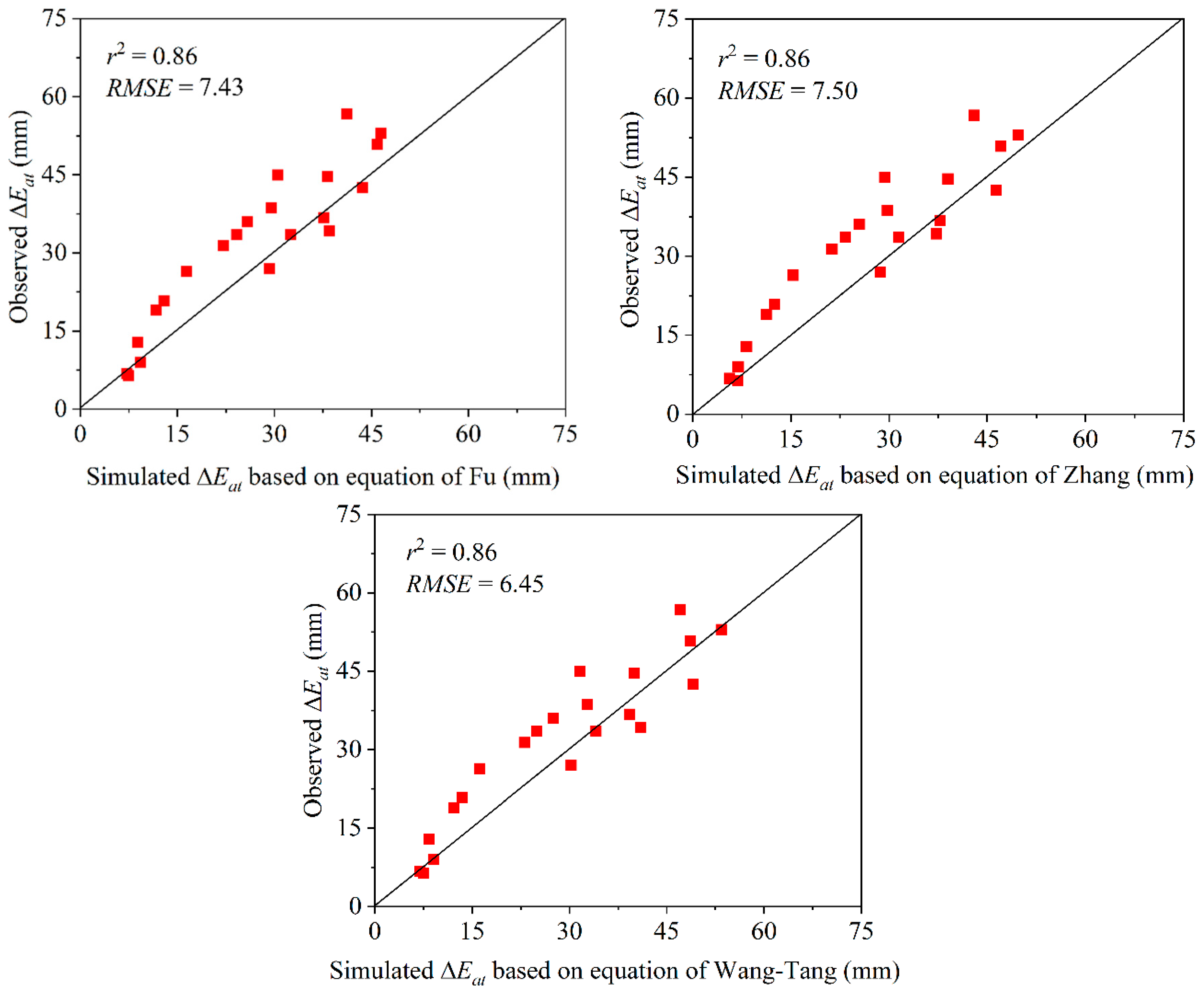
The stepwise linear regression method showed that combining three basic climatic factors and NDVI_t can well explain the changes in the basin-specific n_t in the Budyko-type equations, with r² values between the modeled ${\mathrm{n}}_{\mathrm{t}}^{\prime }$ and n_t calculated based on the Budyko-type equations using observations all being greater than 0.78. This finding indicated that the time-varying n_t proposed in this study yielded better performance of the modeling E_at than a constant n_t in the study area.

(3)

Based on the elasticity and contribution analyses of E_at, it was found that P_t, NDVI_t and T_maxt are the major driving forces to the E_at variations in the study area, and they contributed the most to the E_at variations. During the study period, climate change contributed (whose average contribution is 149.6%) more to $\Delta {\mathrm{E}}_{\mathrm{a}\mathrm{t}}$ than vegetation change (whose contribution rate is −49.4%). Furthermore, the results also indicate that in addition to climatic factors, considering the impacts of vegetation coverage variation on actual evapotranspiration and the water cycle is very important in the study area.

References

1. Huntington, T.G. Evidence for intensification of the global water cycle: Review and synthesis. J. Hydrol. 2006, 319, 83–95. [Google Scholar] [CrossRef]
2. Jung, M.; Reichstein, M.; Ciais, P.; Seneviratne, S.I.; Sheffield, J.; Goulden, M.L.; Bonan, G.; Cescatti, A.; Chen, J.; De Jeu, R.; et al. Recent decline in the global land evapotranspiration trend due to limited moisture supply. Nature 2010, 467, 951–954. [Google Scholar] [CrossRef] [PubMed]
3. Martens, B.; Waegeman, W.; Dorigo, W.A.; Verhoest, N.E.C.; Miralles, D.G. Terrestrial evaporation response to modes of climate variability. NPJ Clim. Atmos. Sci. 2018, 1, 1–7. [Google Scholar] [CrossRef]
4. McVicar, T.R.; Roderick, M.L.; Donohue, R.J.; Niel, T.G.V. Ecohydrology bearings- invited commentary-less bluster ahead? Ecohydrological implications of global trends of terrestrial near-surface wind speeds. Ecohydrology 2012, 5, 381–388. [Google Scholar] [CrossRef]
5. Douville, H.; Ribes, A.; Decharme, B.; Alkama, R.; Sheffield, J. Anthropogenic influence on multidecadal changes in reconstructed global evapotranspiration. Nat. Clim. Chang. 2013, 3, 59–62. [Google Scholar] [CrossRef]
6. Goyal, R.K. Sensitivity of evapotranspiration to global warming: A case study of arid zone of Rajasthan (India). Agric. Water Manag. 2004, 69, 1–11. [Google Scholar] [CrossRef]
7. Roderick, M.L.; Farquhar, G.D. The cause of decreased pan evaporation over the past 50 years. Science 2002, 298, 1410–1411. [Google Scholar]
8. Roderick, M.L.; Rotstayn, L.D.; Farquhar, G.D.; Hobbins, M.T. On the attribution of changing pan evaporation. Geophys. Res. Lett. 2007, 34, 1–6. [Google Scholar] [CrossRef] [Green Version]
9. Wang, K.; Dickinson, R.E. A Review of Global Terrestrial Evapotranspiration: Observation, Modeling, Climatology, and climatic Variability. Rev. Geophys. 2012, 50, 1–54. [Google Scholar] [CrossRef]
10. Wu, J.; Kutzbach, L.; Jager, D.; Wille, C.; Wilmking, M. Evapotranspiration dynamics in a boreal peatland and its impact on the water and energy balance. J. Geophys. Res. Biogeosciences 2010, 115, 1–18. [Google Scholar] [CrossRef] [Green Version]
11. Budyko, M.I. Climate and Life; Academic Press: San Diego, CA, USA, 1974. [Google Scholar]
12. Yang, D.; Sun, F.; Liu, Z.; Cong, Z.; Ni, G.; Lei, Z. Analyzing spatial and temporal variability of annual water-energy balance in nonhumid regions of China using the Budyko hypothesis. Water Resour. Res. 2007, 43, 1–12. [Google Scholar] [CrossRef]
13. Jiang, C.; Xiong, L.; Wang, D.; Liu, P.; Guo, S.; Xu, C.Y. Separating the impacts of climate change and human activities on runoff using the Budyko-type equations with time-varying parameters. J. Hydrol. 2015, 522, 326–338. [Google Scholar] [CrossRef]
14. Brutsaert, W.; Stricker, H. An advection-aridity approach to estimate actual regional evapotranspiration. Water Resour. Res. 1979, 15, 443–450. [Google Scholar] [CrossRef]
15. Brutsaert, W. A generalized complementary principle with physical constraints for land-surface evaporation. Water Resour. Res. 2015, 51, 8087–8093. [Google Scholar] [CrossRef] [Green Version]
16. Liu, X.; Liu, C.; Brutsaert, W. Regional evaporation estimates in the eastern monsoon region of China: Assessment of a nonlinear formulation of the complementary principle. Water Resour. Res. 2016, 52, 9511–9521. [Google Scholar] [CrossRef]
17. Zhang, K.; Kimball, J.S.; Nemani, R.R.; Running, S.W.; Hong, Y.; Gourley, J.J.; Yu, Z. Vegetation Greening and Climate Change Promote Multidecadal Rises of Global Land Evapotranspiration. Sci. Rep. 2015, 5, 1–9. [Google Scholar] [CrossRef]
18. Feng, X.; Fu, B.; Piao, S.; Wang, S.; Ciais, P.; Zeng, Z.; Lü, Y.; Zeng, Y.; Li, Y.; Jiang, X.; et al. Revegetation in China’s Loess Plateau is approaching sustainable water resource limits. Nat. Clim. Chang. 2016, 6, 1019–1022. [Google Scholar] [CrossRef]
19. Dirmeyer, P.A.; Gao, X.; Zhao, M.; Guo, Z.; Oki, T.; Hanasaki, N. GSWP-2: Multimodel analysis and implications for our perception of the land surface. Bull. Am. Meteorol. Soc. 2006, 87, 1381–1397. [Google Scholar] [CrossRef] [Green Version]
20. Lawrence, D.M.; Thornton, P.E.; Oleson, K.W.; Bonan, G.B. The Partitioning of Evapotranspiration into Transpiration, Soil Evaporation, and Canopy Evaporation in a GCM: Impacts on Land–Atmosphere Interaction. J. Hydrometeorol. 2007, 8, 862–880. [Google Scholar] [CrossRef]
21. Yang, D.; Shao, W.; Yeh, P.J.F.; Yang, H.; Kanae, S.; Oki, T. Impact of vegetation coverage on regional water balance in the nonhumid regions of China. Water Resour. Res. 2009, 45, 1–13. [Google Scholar] [CrossRef] [Green Version]
22. Li, D.; Pan, M.; Cong, Z.; Zhang, L.; Wood, E. Vegetation control on water and energy balance within the Budyko framework. Water Resour. Res. 2013, 49, 969–976. [Google Scholar] [CrossRef]
23. Liang, W.; Bai, D.; Wang, F.; Fu, B.; Yan, J.; Wang, S.; Yang, Y.; Long, D.; Feng, M. Quantifying the impacts of climate change and ecological restoration on streamflow changes based on a Budyko hydrological model in China’s Loess Plateau. Water Resour. Res. 2015, 51, 6500–6519. [Google Scholar] [CrossRef]
24. Shao, Q.; Traylen, A.; Zhang, L. Nonparametric method for estimating the effects of climatic and catchment characteristics on mean annual evapotranspiration. Water Resour. Res. 2012, 48, 1–13. [Google Scholar] [CrossRef]
25. Jaramillo, F.; Prieto, C.; Lyon, S.W.; Destouni, G. Multimethod assessment of evapotranspiration shifts due to non-irrigated agricultural development in Sweden. J. Hydrol. 2013, 484, 55–62. [Google Scholar] [CrossRef] [Green Version]
26. Lane, P.N.J.; Best, A.E.; Hickel, K.; Zhang, L. The response of flow duration curves to afforestation. J. Hydrol. 2005, 310, 253–265. [Google Scholar] [CrossRef]
27. Donohue, R.J.; Roderick, M.L.; McVicar, T.R. On the importance of including vegetation dynamics in Budyko’s hydrological model. Hydrol. Earth Syst. Sci. 2007, 11, 983–995. [Google Scholar] [CrossRef] [Green Version]
28. Donohue, R.J.; Roderick, M.L.; McVicar, T.R. Roots, storms and soil pores: Incorporating key ecohydrological processes into Budyko’s hydrological model. J. Hydrol. 2012, 436, 35–50. [Google Scholar] [CrossRef]
29. Guo, M.; Wu, W.; Zhou, X.; Chen, Y.; Li, J. Investigation of the dramatic changes in lake level of the Bosten Lake in northwestern China. Theor. Appl. Climatol. 2014, 119, 341–351. [Google Scholar] [CrossRef]
30. Abatzoglou, J.T.; Ficklin, D.L. Climatic and physiographic controls of spatial variability in surface water balance over the contiguous United States using the Budyko relationship. Water Resour. Res. 2017, 53, 7630–7643. [Google Scholar] [CrossRef]
31. Shahid, M.; Cong, Z.; Zhang, D. Understanding the impacts of climate change and human activities on streamflow: A case study of the Soan River basin, Pakistan. Theor. Appl. Climatol. 2018, 134, 205–219. [Google Scholar] [CrossRef]
32. Jaramillo, F.; Cory, N.; Arheimer, B.; Laudon, H.; Van Der Velde, Y.; Hasper, T.B.; Teutschbein, C.; Uddling, J. Dominant effect of increasing forest biomass on evapotranspiration: Interpretations of movement in Budyko space. Hydrol. Earth Syst. Sci. 2018, 22, 567–580. [Google Scholar] [CrossRef] [Green Version]
33. Xing, W.; Wang, W.; Shao, Q.; Yong, B. Identification of dominant interactions between climatic seasonality, catchment characteristics and agricultural activities on Budyko-type equation parameter estimation. J. Hydrol. 2018, 556, 585–599. [Google Scholar] [CrossRef]
34. Milly, P.C.D. Climate, soil-water storage, and the average annual water-balance. Water Resour. Res. 1994, 30, 2143–2156. [Google Scholar] [CrossRef]
35. Fu, B.P. The calculation of the evaporation from land surface. Sci. Atmos. Sin. 1981, 5, 23–31. [Google Scholar]
36. Zhang, L.; Dawes, W.R.; Walker, G.R. Response of mean annual evapotranspiration to vegetation changes at catchment scale. Water Resour. Res. 2001, 37, 701. [Google Scholar] [CrossRef]
37. Wang, D.; Tang, Y. A one-parameter Budyko model for water balance captures emergent behavior in darwinian hydrologic models. Geophys. Res. Lett. 2014, 41, 4569–4577. [Google Scholar] [CrossRef] [Green Version]
38. Zhang, L.; Hickel, K.; Dawes, W.R.; Western, A.W.; Chiew, F.H.S.; Briggs, P.R. A rational function approach for estimating mean annual evapotranspiration. Water Resour. Res. 2004, 40, 1–14. [Google Scholar] [CrossRef]
39. Liu, Q.; McVicar, T.R.; Yang, Z.; Donohue, R.J.; Liang, L.; Yang, Y. The hydrological effects of varying vegetation characteristics in a temperate water-limited basin: Development of the dynamic Budyko-Choudhury-Porporato (dBCP) model. J. Hydrol. 2016, 543, 595–611. [Google Scholar] [CrossRef]
40. Tian, L.; Jin, J.; Wu, P.; Niu, G. Quantifying the impact of climate change and human activities on streamflow in a Semi-Arid watershed with the Budyko equation incorporating dynamic vegetation information. Water 2018, 10, 1781. [Google Scholar] [CrossRef] [Green Version]
41. Pike, J.C. The estimation of annual runoff from meteorological data in a tropical climate. J. Hydrol. 1964, 2, 116–123. [Google Scholar] [CrossRef]
42. Yang, H.; Yang, D.; Lei, Z.; Sun, F. New analytical derivation of the mean annual water-energy balance equation. Water Resour. Res. 2008, 44, 1–9. [Google Scholar] [CrossRef]
43. Yang, H.; Yang, D. Derivation of climate elasticity of runoff to assess the effects of climate change on annual runoff. Water Resour. Res. 2011, 47, 1–12. [Google Scholar] [CrossRef]
44. Xu, X.; Yang, D.; Yang, H.; Lei, H. Attribution analysis based on the Budyko hypothesis for detecting the dominant cause of runoff decline in Haihe basin. J. Hydrol. 2014, 510, 530–540. [Google Scholar] [CrossRef]
45. Wang, W.; Zou, S.; Shao, Q.; Xing, W.; Chen, X.; Jiao, X.; Luo, Y.; Yong, B.; Yu, Z. The analytical derivation of multiple elasticities of runoff to climate change and catchment characteristics alteration. J. Hydrol. 2016, 541, 1042–1056. [Google Scholar] [CrossRef]
46. Allen, R.G.; Pereira, L.S.; Raes, D.; Smith, M. Crop evapotranspiration-Guidelines for computing crop water requirements-FAO Irrigation and drainage paper 56. FAO Rome 1998, 300, D05109. [Google Scholar]
47. Djaman, K.; Koudahe, K.; Lombard, K.; O’Neill, M. Sum of Hourly vs. Daily Penman-Monteith Grass-Reference Evapotranspiration under Semiarid and Arid Climate. Irrig. Drain. Syst. Eng. 2018, 7. [Google Scholar]
48. Djaman, K.; Ndiaye, P.M.; Koudahe, K.; Bodian, A.; Diop, L.; O’Neill, M.; Irmak, S. Spatial and temporal trend in monthly and annual reference evapotranspiration in Madagascar for the 1980–2010 period. Int. J. Hydrol. 2018, 2, 110–120. [Google Scholar] [CrossRef] [Green Version]
49. Tucker, C.J.; Pinzon, J.E.; Brown, M.E.; Slayback, D.A.; Pak, E.W.; Mahoney, R.; Vermote, E.F.; El Saleous, N. An extended AVHRR 8-km NDVI dataset compatible with MODIS and SPOT vegetation NDVI data. Int. J. Remote Sens. 2005, 26, 4485–4498. [Google Scholar] [CrossRef]
50. Xiong, L.; Guo, S. Appraisal of Budyko formula in calculating long-term water balance in humid watersheds of southern China. Hydrol. Process. 2012, 26, 1370–1378. [Google Scholar] [CrossRef]
51. Gilroy, K.L.; McCuen, R.H. A nonstationary flood frequency analysis method to adjust for future climate change and urbanization. J. Hydrol. 2012, 414–415, 40–48. [Google Scholar] [CrossRef]
52. Mann, H.B. Non-parametric tests against trend. Econometrica 1945, 13, 245–259. [Google Scholar] [CrossRef]
53. Kendall, M.G. Rank Correlation Measure; Charles Griffin: London, UK, 1975. [Google Scholar]
54. Yue, S.; Pilon, P.; Cavadias, G. Power of the Mann-Kendall and Spearman’s rho tests for detecting monotonic trends in hydrological series. J. Hydrol. 2002, 259, 254–271. [Google Scholar] [CrossRef]
55. Yue, S.; Wang, C.Y. Applicability of prewhitening to eliminate the influence of serial correlation on the Mann-Kendall test. Water Resour. Res. 2002, 38, 4. [Google Scholar] [CrossRef]
56. Alexander, L.V.; Allen, S.K.; Bindoff, N.L.; Bréon, F.-M.; Church, J.A.; Cubasch, U.; Emori, S.; Forster, P.; Friedlingstein, P.; Gillett, N.; et al. Climate change 2013: The physical science basis, in contribution of Working Group I (WGI) to the Fifth Assessment Report (AR5) of the Intergovernmental Panel on Climate Change (IPCC). Science 2013, 129, 83–103. [Google Scholar]
57. Ding, Y.; Ren, G.; Shi, G.; Gong, P.; Zheng, X.; Zhai, P.; Zhang, D.; Zhao, Z.; Wang, S.; Wang, H.; et al. National assessment report of climate change (I): Climate change in China and its future trend. Adv. Clim. Chang. Res. 2006, 2, 3–8. [Google Scholar]
58. McVicar, T.R.; Roderick, M.L.; Donohue, R.J.; Li, L.T.; Van Niel, T.G.; Thomas, A.; Grieser, J.; Jhajharia, D.; Himri, Y.; Mahowald, N.M.; et al. Global review and synthesis of trends in observed terrestrial near-surface wind speeds: Implications for evaporation. J. Hydrol. 2012, 416–417, 182–205. [Google Scholar] [CrossRef]
59. Zhang, L.; Potter, N.J.; Zhang, Y. Water balance modeling over variable time scales based on the Budyko framework—Model development and testing. J. Hydrol. 2008, 390, 121–122. [Google Scholar] [CrossRef]
60. Koudahe, K.; Djaman, K.; Adewumi, J.K. Evaluation of the Penman–Monteith reference evapotranspiration under limited data and its sensitivity to key climatic variables under humid and semiarid conditions. Model. Earth Syst. Environ. 2018, 4, 1239–1257. [Google Scholar] [CrossRef]
61. Yang, H.; Yang, D.; Hu, Q. An error analysis of the Budyko hypothesis for assessing the contribution of climate change to runoff. Water Resour. Res. 2014, 50, 9620–9629. [Google Scholar] [CrossRef]
62. Li, M.; Chu, R.; Shen, S.; Islam, A.R.M.T. Dynamic analysis of pan evaporation variations in the Huai River Basin, a climate transition zone in eastern China. Sci. Total Environ. 2018, 625, 496–509. [Google Scholar] [CrossRef]
Figure 1. Map of the study area and locations of meteorological and hydrological stations used in this study.
Water 12 00508 g001
Figure 2. Changes in climatic variables and the Normalized Difference Vegetation Index (NDVI) in the NSPB. (af) are the changes in precipitation (P), temperature term, relative humidity (RH), sunshine duration (S), wind speed at a height of 2 m (u2) and NDVI, respectively. The value of “ZMK” is the trend of the variable over the period of 1982–2013 estimated using the nonparametric trend-free pre-whitening Mann–Kendall trend test. The symbol ‘*’ after ZMK indicates that the estimated trend is significant at the 0.05 significance level (i.e., p-value < 0.05). The black lines represent the annual time series of variables, the blue lines represent the linear trends of the annual time series of variables and the red lines represent the 11-year moving averages of the annual time series of variables.
Water 12 00508 g002
Figure 3. Comparison between the parameter n t for each Budyko-type equation estimated by Equations (11a)–(11c) and nt derived from the Budyko-type equations using the observations. RMSE = root mean squared error.
Water 12 00508 g003
Figure 4. Comparison of Eat calculated from the water balance equation (black triangles) and the simulated Eat from the cases when the parameter nt in each Budyko-type equation is treated as a constant (red lines) and when the value of parameter nt is estimated using Equations (11a)–(11c) (blue lines). (ac) are for the Budyko-type equations of Fu [35], Zhang et al. [36] and Wang-Tang [37], respectively.
Water 12 00508 g004aWater 12 00508 g004b
Figure 5. Comparison of simulate Δ E a t with Equation (12) and the observed values in each post-change time window.
Water 12 00508 g005