Short-Term Optimal Operation of Baluchaung II Hydropower Plant in Myanmar

Abstract

The short-term optimal operation model discussed in this paper uses the 2016 to 2018 daily and monthly data of Baluchaung II hydropower station to optimize power generation by minimizing water consumption effectively in order to get more revenue from optimal operation. In the first stage, run-off-river type Baluchaung II hydropower station data was applied in a mathematical model of equal micro-increment rate method for optimal hydropower generation flow distribution unit results. In the second stage, dynamic programming was used to get optimal hydropower generation unit distribution results. The resultant data indicated that optimized results can effectively guide the actual operation run of this power station. The purpose of the optimal load dispatching unit was to consider the optimal power of each unit for financial profit and numerical programming on the actual data of Baluchaung II hydropower plant to confirm that our methods are able to find good optimal solutions which satisfy the objective values of 17.75% in flow distribution units and 24.16% in load distribution units.

1. Introduction

Water is used for many purposes such as drinking, cleaning, irrigation, power generation, recreation, and navigation. It is vital for all living things and also for infrastructure, industrialization, and urbanization of the country. In recent years, global warming has threatened the ecosystems of the earth that affects the daily obtainable water resources. If it is handled well with better technologies, flood and drought can be better controlled. Optimal water usage is becoming essential to protect water shortages in the dry season particularly in arid and semi-arid regions because obtainability of enough water resources and cost effectiveness of water usage impacts the management of hydropower generation. Hydropower generation is mostly affected by physical and economic factors. Physical factors depend on high flow rate from reservoirs, waterfalls and lakes, as well as dam reinforcement, flexible weather conditions, and silt-free water. Meanwhile, economic factors, power demand, capital investment, and lack of energy sources are the main factors for better power generation. Reckoning the costs of operating numbers of turbines, dams, intake, pipelines, fore bays, penstocks, powerhouses, protection, regulation, control, network connections, and transmission lines also supports the economic profit of hydropower plant [1].

The optimal operation of a hydropower station is to generate load with many constraints for many purposes [2]. There are many algorithms for mathematical models to optimize operation with correctly conceptualized theories and formulas [3]. In designing a model, there are two methods used: optimization and simulation [4,5,6]. A simulation model is a descriptive model that tries to express the actual system of operation characteristics by using the complicated interrelations between components. Even though the model is easy and flexible to use, it needs much experimentation in hydropower-related applications. An optimization model is a normative model which attempt to get the utmost finest solution with the multiple suitable constraints. In fitting the structure and format of mathematical algorithm, these models have more limitations than simulation models.

There are three types of period to optimize the operation: short term which schedules for one to two weeks, medium term that programs for 3 to 18 months and long term for one to five years. The main goal of optimization of hydropower station is in order to meet the requirements of relevant departments of national economy and society according to above-mentioned principles of operation with certain optimization theories and methods. This means to optimize the power generation in order to get stable and economical in load balancing with the utmost total direct and indirect benefits. Direct benefit is concerned with the primary operation benefit got from the power generation operation dispatching for the national load demand. Indirect benefits relates to the social and ecological impacts got from controlling the power generation, navigation, irrigation, flood control, and urban water supply.

Therefore, the reason for conducting short-term optimal operation of Baluchaung II hydropower station in Myanmar is to optimize the power generation by minimizing water consumption and evaluate the optimal flow and load distribution units by equal micro-increment rate method and dynamic programming. The calculation data are from the Baluchaung II hydropower station in Myanmar with the installed capacity of 168 MW (28 MW × 6). It is a run-off-river type hydropower station that supplies the national electricity demand as a base load power station in Myanmar. Unfortunately, although there are plenty of papers about hydropower status reports, there is a few technical papers about optimal operation relating to reservoirs and flood control in Myanmar. Therefore, this paper can be helpful to manage the hydropower plant for optimal operation. Many scholars have researched how to use water efficiently in optimal design, planning, and operation in economics and engineering fields.

The application of the researched methods depends on the characteristics of the different types of hydropower stations. Methods are classified into two main groups: heuristic and mathematical programming. Heuristic methods include improving particle swarm optimization [7,8,9], progressive optimal algorithms [10,11], improved progressive optimal algorithm [12], chaos cultural sine cosine algorithm [13], and recursive optimization [14]. Mathematical programming includes linear programming [15], mixed integer linear programming [16], stochastic programming, and dynamic programming. Hybrid algorithms give better results and are more accurate than single algorithms and the key limitation of them is that they cannot improve the results very much more than actual operation.

From the above literature, it can be noted that the purpose of short-term optimal operation is to regulate the water flow hour-by-hour in order to stabilize the scheduling periods for the peak hours of the day and forecast the daily run-off between the conditions of multi-constraints in a complex system. Due to complex multi-constraints between water level and output in modelling of hydro power stations, feasibility of scheduling methods is still needed to improve on practical operations, and more new hybrid algorithms need to be considered for future optimization issues. Also, in actual power generation, the load demand changes need to be taken into account because they are a main factor of the instability of load distribution units. Some research papers give general conclusions and do not clearly point out the advantages and the differences between the results. In short-term load dispatching problems, dynamic programming is a better method because of steady computational processes in finding optimal solutions. Therefore, dynamic programming is used in this paper in order to get better optimal results in the case of load swinging.

2. Case Study

2.1. Baluchaung II Hydropower Plant

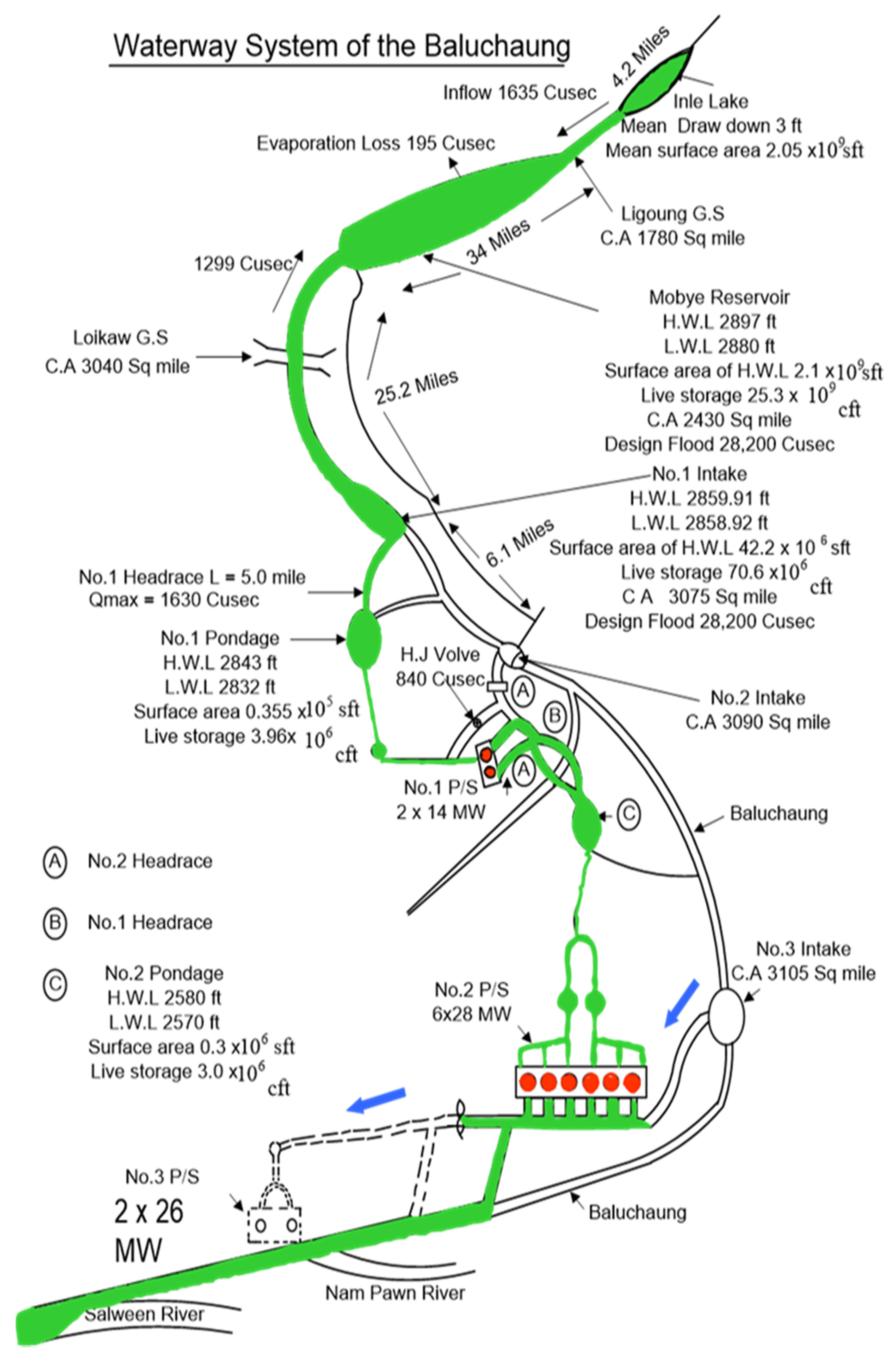
Myanmar is a Southeast Asian country which depends mainly on its water resources for electricity supply. Although it is implementing many hydropower stations for the country’s needs, problems of electricity shortage are still encountered during the summer season. Therefore, maximum load with minimum water usage is the aim for hydropower plants in Myanmar in order to optimize the load distribution of the generator units. Most of the hydropower plants in Myanmar are the reservoir type and some are run-off river type. They are essential to produce electricity which requires no fuel and are much simpler to operate and maintain than other types of power station due to lower operating costs. The total cost of run-off river power plants mainly rely on the number of turbines [17]. The power capacity of a hydropower plant is primarily the function of two variables: flow rate expressed in cubic meters per second and the hydraulic head, which is the elevation distance the water falls in passing through the power plant. A typical hydropower plant can be classified according to rated power capacity, type of turbine, water head, and location and type of dam as well as sizes which includes large, small, micro, and pico, depending on generated MW. The basic components of hydropower plants are intake, dam, headrace, fore bay, penstock, power house, turbine, generator, and tailrace. Baluchaung II hydroelectric power station is located in Loikaw which is the Southern Shan state and it generates power from the Baluchaung River, a tributary of the Thanlwin River, which is located in the Middle East region of Myanmar. The water enters to the Baluchaung River from the Mobye Reservoir which collect water from the Inle Lake. The construction of the Baluchaung II power station was divided into two phases. Investigations were started in 1954 and construction was started in 1960 for the first three generator (28 MW × 3) as a Japanese post-war reparation project. The second-phase (28 MW × 3) followed in the period between 1970 and 1974 and was self-funded. The power house has six units of turbine generators. Units 1 to 3 were constructed during the first stage construction and units 4 to 6 were constructed as the second stage. All turbines are horizontal Pelton type turbines that have two runners with twenty buckets on the both side of the generator combined by the main shaft and the each runner receives a water jet from two nozzles and has two horizontal shaft rotary inlet valves. The maximum capacity is 168 MW, maximum discharge is 47.58 m³/s, total head is 436.6 m and effective head is 416.5 m. The generated power is transported to the Yangon and Mandalay regions via 230 kV and 132 kV transmission lines. The power station has been supplying more than 50% of the total electric power of Myanmar for the past 40 years. The facility capacity and the output of electric power have been 20% and 40%, respectively, of the total in Myanmar in last two decades and therefore, it was very important for country’s electricity needs because it was the first large-scale hydropower plant established and it is always considered as the base load power plant especially in dry season. The Ministry of Electricity and Energy aims to implement a Myanmar electricity master plan to generate 100 percent electricity with the energy generation mix of 5% solar and wind, 8% natural gas, 30% coal and hydropower more than half of electricity in 2030. The national economy depends on electricity, peace, and human resources. Therefore, trying to get access electricity for the 22 million population is the country’s goal as a developing country. The optimal operation of hydropower plant and waterway system of Baluchaung II hydropower station is described in the Figure 1.

2.2. Methodology

The methodology includes three parts. The first part introduces the optimal operation of hydropower plant. The second part is about the equal micro-increment rate method and the third part explains the dynamic programming method. The equal micro-increment rate method was used for programming the results of optimal hydropower generation flow and the dynamic programming method was used for hydropower generation. The objective of this paper is to optimize the hydropower station in the unit and hydropower generation level and to upgrade the efficiency in the higher stage.

Establishment of the Optimal Operation Model in the Plant

The basic task of the optimal operation of the hydropower station is to rationally arrange the load distribution of the units [18,19]. These units are put into operation on the basis of the known power generation flow or output of the hydropower station to achieve the highest power generation efficiency of the whole plant and increase the economic benefits of the hydropower station. The following principles should be followed when conducting research on the optimal operation of the plant.

(1) Optimization principle.

The economic operation of the plant can adopt different economic principles according to different situations. When the power generation flow of the power station is given in the “water to electricity” mode, the power station maximizes its output by optimizing the unit commitment and water distribution. When the load of the power station is given in the “electricity to water” mode, the power station minimizes its power generation water consumption by optimizing the unit commitment and load distribution.

(2) Principles for safe operation of power stations and units.

When the unit is running in certain output and head areas, severe vibrations will occur. This is called the vibration zone. Vibration is a resonance phenomenon caused by mechanical, hydraulic, and electromagnetic vibrations, which seriously threaten the safe production of the power station and the service life of the unit. Therefore, the optimal operation of the plant should avoid the vibration zone operation.

According to the actual production of “electricity to water” mode by Baluchaung II hydropower station, this paper uses the minimum water consumption as the optimization criterion to establish the optimal operation model of the plant. The objective function is as follows:

$$Q=\min {\displaystyle \sum _{i=1}^n{Q}_i(N_i,H)}$$

(1)

where Q is the total power generation flow of the hydropower station, i is the unit number, N_i is the output of the unit I, H is the water head, Q_i (N_i, H) is the power generation flow when the unit N_i is output, and the head is H.

The constraint condition is the balance of output force. Equation (2) explains the constraints of power output. It should be noted that after many years of operation, the Baluchaung II hydropower station is in good running condition and there is no serious vibration of the unit. Therefore, the model does not consider the vibration zone constraint.

$$\{\begin{array}{l}{\displaystyle \sum _{i=1}^n{N}_i}=N\\ N_{\min }(H)\le N_i\le N_{\max }(H)\end{array}$$

(2)

In the formula, N_min(H) and N_max(H) are the lower limit and upper limit of the output of unit i when the head is H.

2.3. Equal Micro-Increment Rate Method for Model Solving

Hydropower station economic operation model-solving methods are generally divided into two categories. One is the traditional method, which mainly refers to the graphical method using the flow increase rate characteristic curve and the flow characteristic curve, the most representative method of equal micro-increment rate. The other is mathematical optimization methods, mainly other modern mathematical methods such as dynamic programming. The principle of the micro-increment rate method is easy and the calculation is simple. The flow characteristics of the unit of Baluchaung II hydropower station that meet the requirements of the micro-increment rate method must be in the condition of a smooth and convex curve. Therefore, the method of solving for the Baluchaung II hydropower station is the equal-increment rate method economic operation model and dynamic programming. When solving the objective function corresponding to Equation (3), the Lagrangian function F can be constructed:

$$F={\displaystyle \sum _{i=1}^n{Q}_i+\lambda (N-{\displaystyle \sum _{i=1}^n{N}_i})}$$

(3)

The necessary conditions for F to reach the extreme point are:

$$\{\begin{array}{l}\frac{\partial F}{\partial N_1}=\frac{\partial Q_1}{\partial N_1}-\lambda =0\\ \frac{\partial F}{\partial N_2}=\frac{\partial Q_2}{\partial N_2}-\lambda =0\\ ⋮\\ \frac{\partial F}{\partial N_n}=\frac{\partial Q_n}{\partial N_n}-\lambda =0\end{array}$$

(4)

To express the flow rate of micro-increment of the i-th unit when the unit is fixed, Equation (5) can be expressed as:

$$q_1=q_2=q_3=q_n=\frac{1}{\lambda }=constant$$

(5)

Equation (5) is the principle of the micro-increment rate of the optimal flow distribution between the operating units. When the unit models in the hydropower station are the same, that is, the micro-increment rate curves of the units are the same, the calculation result of the micro-increment rate method is the average load of the power station which is evenly distributed to each unit that is put into operation. At this time, the key to the optimal operation of the plant is to determine the number of units that are put into operation. Therefore, when solving the economic operation model of the Baluchaung II hydropower station when the total output of the power station is certain, one to six units of known data are required to calculate the situation and select the scheme with the smallest total power generation flow.

2.4. Dynamic Programming

Dynamic Programming (DP) is a traditional method like linear and non-linear programming introduced by Richard Bellman in 1950s for multiple purposes like applications for economics, engineering, and also in the army [20]. It is used not only in mathematics but also in computer programming. To calculate successfully, the order of the sequence is from the beginning state to final state. The optimization principle can be expressed as the optimal decision sequence from the initial state and initial decision of the process to the next decision state. Well known DP algorithms are Unix diff for comparing two files, Bellman-Ford for shortest path routing in networks, and TeX, the ancestor of LaTeX for score predictor. The advantage of DP is getting final results by memorization to avoid repetitive work. Two types of DP problems are optimization and combinatorial. These can used in two approaches: top-down and bottom-up approaches. The calculation steps of DP are establishment of dynamic programming recursion equation, recursive calculation, and real-time economic operation plan formulation. These are shown below.

2.4.1. Stage and Stage Variables

For real-time economic operation problems, each unit can be staged and put into the unit. The number i represents the phase variable (i = 1, 2,…, n). i is the unit stage, and 1~(i − 1) is the remaining period.

2.4.2. State Variables

State variables are the total output of 1~i units $P_i\sum (t) \left(i=0,1,\dots ,n\right)\mathrm{where} P_o\sum (t)$ = 0 as the i-th order selecting and it needs to describe the evolution of the process with no after-effects.

2.4.3. Decision Variables

Decision variables are the output P_i (t) of each unit, and the t-time (segment) of the i-th unit. If the force range composition allows the decision set D_i (t), then P_i(t) ∈ D_i(t). The sub-strategy is recorded as: $U_i=\left\{P_1\left(t\right), P_2\left(t\right)\dots ., P_i\left(t\right)\right\}.$

2.4.4. State Transition Equation

In the state transition equation the any stage (unit) i, describes the end state $P_i\sum \left(t\right)$ with stage initial state $P\left(i-1\right)\sum$(t) for any stage unit i. The mathematical relationship between the decision and the decision P_i(t) is called the state transition equation, and the load balance equation of the model is the state transition

$$P_i\sum \left(t\right)=P_{i-1}\sum \left(t\right)+P_i\left(t\right)$$

(6)

For this deterministic decision process, the state of the next phase is completely determined by the state and decision of the time period.

2.4.5. Index Function and Optimal Value Function

In its function, the power flow $Q{ }_i\left(P{ }_i\left(t\right)\right)$ of the i-th stage represents the index function, 1~i. The optimal value of the total power generation flow in the stage $Q_i{}^{*}((P_i \sum \left(t\right))$ represents the optimal value function.

$$Q_i(P_i\left(t\right))= Q_i(P_i\left(t\right), H\left(t\right))$$

(7)

$$Q_i{}^{*}(P_i\sum \left(t\right))=mi{n}_{ui}\{\sum _{j=1}^{i}Qi\left(Pj\left(t\right)\right)\}$$

(8)

2.4.6. Recursive Equation

According to the multi-stage decision principle and Equations (7) and (8), the following sequence recursion can be listed

$$\begin{array}{c}\{\begin{array}{c}{Q}_i{}^{*}(P_i\sum \left(t\right)\\ Q_o{}^{*}\left(0\right)=0\end{array}= \end{array}\begin{array}{c}min\\ P_i\left(t\right)\in D_i\left(\mathrm{t}\right)\end{array}\{Q_i(P_i\left(t\right), H\left(t\right)) + Q_{i-1}{}^{*} (P_i\sum \left(t\right)-P_i\left(t\right))\}\begin{array}{c}\left(i=1~n\right)\\ \begin{array}{c}\left(i=0\right)\end{array}\end{array}$$

(9)

2.4.7. Constraints

The constraint in the recursive calculation is mainly the unit output limitation of Equations (10) and (11) which are used in the back-calculation to determine the optimal decision.

$$(P_i{}^{\min }\left(t\right)\le (P_i\left(t\right)) \le { }_{ }{P}_i{}^{\max }\left(t\right))$$

(10)

$$\sum _{i=1}^n{P}_i\left(t\right)=P_s\left(t\right)$$

(11)

3. Calculation and Discussion

In the calculation steps, Microsoft excel was used to sort out the average power generation flow rate and generation output for each month from the 2016 to 2018 data. Then, the unit characteristics curve was fixed by exponential curves and the unit dynamic characteristic curve compared with other power plant performance curves such as the upstream water level capacity curve, and downstream water level flow curve [21]. C# software was used to write the program for optimal generation flow and actual generation flow from the known data of six units from Baluchaung II hydropower station. The equal micro-increment rate method was used for calculation. The dynamic programming method was applied for optimal and actual power generation and the results compared to get the better optimal solution.

3.1. Unit Characteristic Curve Fitting

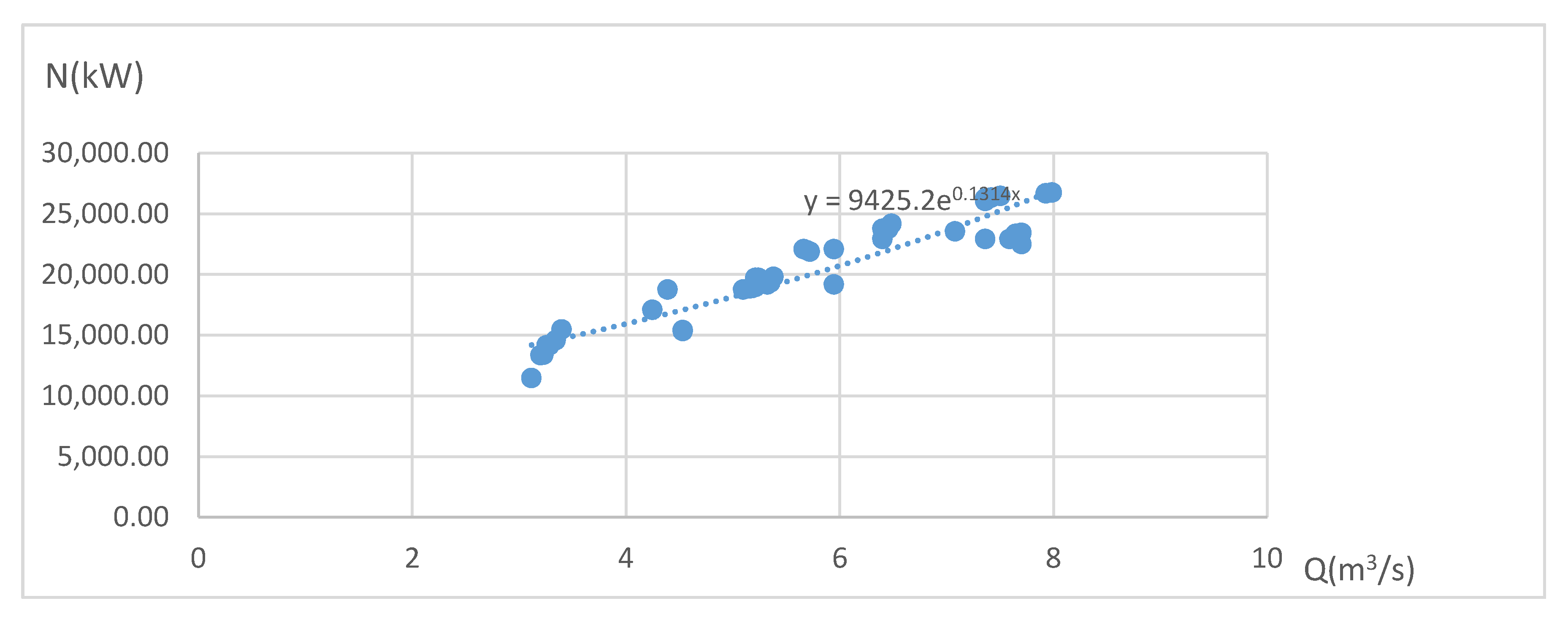
The Baluchaung II hydropower station is a run-off-river power station. This is why the upstream water level and the downstream water level of the power station remain unchanged and the power head is constant at 1388 feet. Therefore, the upstream water level storage capacity curve and the downstream water level flow curve are not required for the model solution. The unit dynamic characteristic curve which is the NQ curve (which should have been the NQH curve, but reduced to the NQ curve since H has been determined to constant head) is required to find out the optimal operation [22]. The Baluchaung II hydropower station has six identical units, and its unit characteristic curve is basically the same, but due to the reasons that may not be provided by the manufacturer, or the fact that the theoretical curve may not match the actual operation, there is no suitable model for solving the problem of unit dynamic characteristic curve. Therefore, this paper uses the measured data in the historical running process to perform curve fitting.

Table 1. Measured data of Baluchaung II hydropower station.

Date	Q	Unit						E	Average E	Total	Net Total Transmission
		1	2	3	4	5	6
1.Mar.2016	1202	599	584	591	596	607	602	3579	149	3555	3550
2.Mar.2016	1201	542	567	567	579	569	536	3361	140	3335	3331
3.Mar.2016	1102	504	529	537	541	550	540	3201	133	3177	3173
4.Mar.2016	1202	488	485	494	541	508	490	3005	125	2982	2978
5.Mar.2016	1202	503	480	494	498	510	464	2948	123	2926	2921
6.Mar.2016	1202	431	402	456	421	468	481	2859	111	2636	2634
7.Mar.2016	1203	513	438	508	477	512	548	3004	125	2981	2976
8.Mar.2016	1104	473	476	471	485	467	475	2847	119	2825	2820
9.Mar.2016	1105	485	450	497	497	507	479	2916	121	2889	2885
10.Mar.2016	1102	461	4545	435	4763	448	451	2726	114	2705	2701

shows the measured data of Baluchaung II hydropower station.

Since the hydropower station runs more than one unit, when the output of each unit is different, it is impossible to determine the corresponding flow rate of each unit under its output. Therefore, in the curve fitting, it is necessary to select a period in which the unit output is relatively close and one day is the time period in this article, such as 27 September 2016. For the selected day, the total output of the hydropower station and the total power generation flow are evenly distributed to each unit as the basic data of curve fitting. From 2016 to 2018, the time period selected meets the requirements and form the basic data set. The basic data set was fitted in logarithmic form, and the curve obtained is shown in Figure 2. The NQ curve relationship was obtained as follows:

$$N=9425.5\times \exp \left(0.1314Q\right)$$

(12)

After fitting the curve, the equal micro-increment method was used to calculate the results of optimal power generation flow and dynamic programming was used to find the optimal power generation. Using the data from 2016 to 2018, the fitting accuracy test was carried out, that is, the power generation flow of each unit was obtained by inversely calculating the power generation flow according to the measured output of each unit, and then the total power generation flow of the hydropower station was calculated, shown in

Table 2. Power generation flow results of Baluchaung II hydropower station.

Months	2016			2017			2018
	Qa (m3/s)	Qo (m3/s)	Efficiency (%)	Qa (m3/s)	Qo (m3/s)	Efficiency (%)	Qa (m3/s)	Qo (m3/s)	Efficiency (%)
Jan	944	845	11%	1935	1774	8%	2011	1910	5%
Feb	1085	974	11%	1973	1835	7%	2079	2018	3%
Mar	1834	1586	13%	1985	1854	7%	2070	2005	3%
Apr	1584	1318	17%	1973	1850	6%	2051	2023	2%
May	1876	1641	12%	2088	2031	3%	2157	2144	1%
June	1757	1522	14%	1718	1604	7%	2017	1913	5%
Jul	1466	1245	15%	1446	1294	11%	2122	2088	2%
Aug	1098	959	12%	1527	1339	13%	2047	1955	5%
Sep	468	398	14%	1001	857	15%	1832	1624	11%
Oct	1115	963	15%	1522	1372	12%	1787	1598	11%
Nov	1058	870	18%	2053	1979	4%	2121	2085	2%
Dec	1498	1274	16%	2105	2064	2%	2103	2082	1%

, and the measured power generation flow rate of the hydropower station was performed. The results are shown in following figures and tables.

3.2. Water Flow Optimization

In the Table 2, Q_a means the actual power generation flow and Q_o means the optimal power generation flow. In contrast, the maximum efficiency of power generation, in November 2016, was 18 percent whereas the lowest, in May 2018, was 1 percent, when the optimal power generation flow was highest at 2144 m³/s. It can be noted that efficiency is higher when the power generation flow is lower. The optimal solution can save over 200 m³/s water in some months whereas in some other literature, the optimized solution could save, at the most, 10 m³/s [6].

In

Table 3. The power generation flow distribution of units in actual and optimal operations.

Date	Actual Power Generation Flow (m3/s)						Optimal Power Generation Flow (m3/s)
	Unit 1	Unit 2	Unit 3	Unit 4	Unit 5	Unit 6	Unit 1	Unit 2	Unit 3	Unit 4	Unit 5	Unit 6
1.Mar. 2016	348	343	346	348	351	349	371	371	371	371	371	183
2.Mar. 2016	329	338	338	342	339	327	371	371	371	371	371	3
3.Mar. 2016	316	325	327	329	332	329	371	371	371	371	319	-
4.Mar. 2016	310	308	312	329	317	310	371	371	371	371	236	-
5.Mar. 2016	315	307	312	313	318	300	371	371	371	371	207	-
6.Mar. 2016	287	275	297	283	302	307	371	371	371	371	152	-
7.Mar. 2016	319	290	317	305	319	331	371	371	371	371	236	-
8.Mar. 2016	304	305	303	309	302	305	371	371	371	371	144	-
9.Mar. 2016	309	295	313	313	317	306	371	371	371	371	188	-
10.Mar. 2016	299	820	289	832	294	295	371	371	371	371	43	-
11.Mar. 2016	302	297	300	304	308	301	371	371	371	371	115	-
12.Mar. 2016	276	276	271	280	275	284	371	371	371	283	/	-
13.Mar.2016	299	289	293	301	298	291	371	371	371	371	17	-
14.Mar.2016	303	294	294	303	271	300	371	371	371	371	6	-
15.Mar.2016	293	287	293	289	313	297	371	371	371	371	27	-

, the actual solution consumes water discharge of 1662 m³/s with six distribution units whereas the optimal solution used water release of 1396 m³/s with four distribution units on 12 March 2016, as highlighted in red. The optimal solution, saved two turbines of water consumption and released a minimum discharge of water. From the calculated results, it can be seen that the lower the water consumption, the more cost-effective the power generation. Therefore, the equal micro-increment rate method gave the best solution for optimal power generation flow, saved at least one turbine of consumption during most days, and consumed less water than the actual operation every day during the three years.

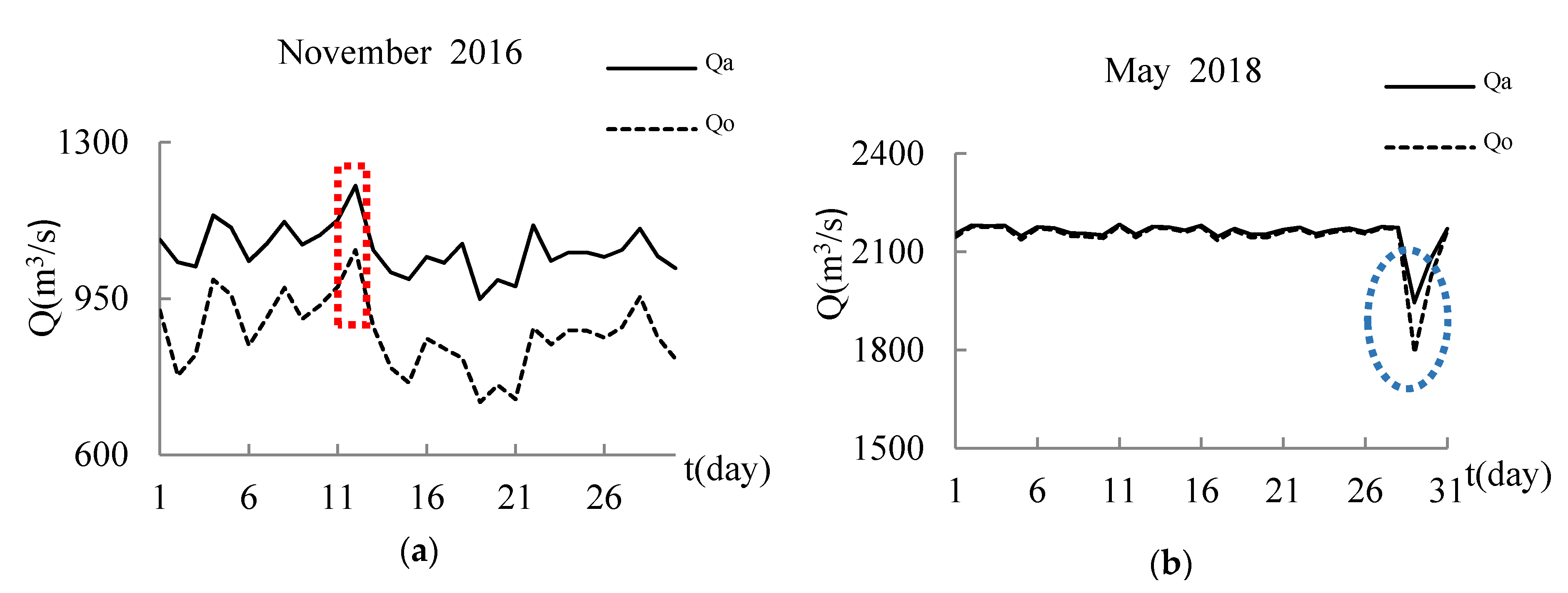
The generation flow curves for 2016 to 2018 are shown in Figure 3. From the calculated results, the solid line curve corresponds to the actual hydropower generation flow, whereas the dotted line curve corresponds to the optimal hydropower generation flow. In November 2016, as shown in Figure 3a, the two curves fluctuated together with a small gap of between 800 m³/s and 1100 m³/s. This means that the two curves were synchronized until the end of the month with the actual power generation curve was higher than the optimal power generation flow showing the use of less water in optimal rather than actual operation and denoting that it was optimal operation. The red dotted rectangular shape shows that water consumption reach its lowest point in November 19 which is 718 m³/s in optimal operation and 949 m³/s in actual operation with the efficiency of 24.3 percent. In Figure 3b, the actual operation curve is the same with optimal operation because both unit generations were similar to each other in May 2018. However, on only one day in May 2018 it dropped to minimum value, where the blue dotted circle which reaches 1791 m³/s in optimal and 1945 m³/s in actual solution and efficiency to 7.9 percent. By comparing two months in Figure 4, it can be seen that the smaller the water flow gets the higher the efficiency in order to get more benefit in power production. From the above calculated curves, it can be noted that the volumetric flow rate cannot be constant as it is changing in each period of time and the results show the optimal solution curves are always lower than actual solution curves because of the optimal resulted values are lower than actual solution to minimize water consumption in order to get more revenue from power generation.

In the

Table 4. Power generation results of Baluchaung II hydropower station.

Month	2016			2017			2018
	Eo	Ea	Efficiency	Eo	Ea	Efficiency	Eo	Ea	Efficiency
Jan	1602	1455	10%	3426	3145	9%	3547	3384	5%
Feb	1873	1678	15%	3493	3251	8%	3669	3566	3%
Mar	3083	2793	11%	3511	3289	7%	3636	3532	3%
Apr	2783	2310	20%	3488	3271	8%	3625	3573	2%
May	3295	2972	11%	3689	3600	3%	3832	3805	1%
June	3099	2677	19%	3029	2816	9%	3564	3383	6%
Jul	2574	2181	19%	2533	2275	13%	3764	3699	2%
Aug	1898	1650	15%	2683	2356	15%	3598	3466	4%
Sep	801	684	10%	1734	1494	16%	3240	2872	13%
Oct	1934	1679	17%	2674	2405	15%	3162	2814	14%
Nov	1852	1493	24%	3518	3512	1%	3780	3715	2%
Dec	2629	2233	20%	3718	3644	2%	3728	3686	1%

, E_a means the actual power generation and E_o means the optimal power generation. From the calculated results of three years, the maximum efficiency of power generation was 24.16 percent and minimum efficiency was 0.72 percent. The lowest optimal power generation was 1851.7 MWH and the highest optimal power generation was 3831.9 MWH which is the full load of five units.

The dynamic programming algorithm bottom-up approach method was used in order to produce the optimal distribution of units which are shown in

Table 5. The load distribution of units in actual and optimal operations.

Date	Actual Power Generation (MWH)						Optimal Power Generation (MWH)
	Unit 1	Unit 2	Unit 3	Unit 4	Unit 5	Unit 6	Unit 1	Unit 2	Unit 3	Unit 4	Unit 5	Unit 6
1.Dec.2018	639	638	641	658	660	657	672	672	672	672	672	545
2.Dec.2018	612	604	558	631	630	622	672	672	672	672	672	359
3.Dec.2018	652	643	645	664	667	664	672	672	672	672	672	576
4.Dec.2018	649	645	646	666	665	663	672	672	672	672	672	576
5.Dec.2018	640	637	640	655	654	647	672	672	672	672	672	525
6.Dec.2018	631	620	632	649	652	645	672	672	672	672	672	486
7.Dec.2018	626	615	636	650	652	646	672	672	672	672	672	486
8.Dec.2018	645	62	645	666	663	662	672	672	672	672	672	35
9.Dec.2018	642	19	632	665	661	658	672	672	672	672	663	-
10.Dec.2018	622	0	626	648	659	626	672	672	672	672	516	-
11.Dec.2018	655	110	655	666	669	661	672	672	672	672	672	88
12.Dec.2018	644	473	643	666	667	663	672	672	672	672	672	415
13.Dec.2018	562	579	638	670	666	666	672	672	672	672	672	441
14.Dec.2018	610	603	530	617	618	612	672	672	672	672	672	307
15.Dec.2018	639	637	646	555	660	656	672	672	672	672	672	450

. Based on actual load distribution of units, the optimal outcomes obtained with 0.1 MWH discrete interval and vibration area does not take into consideration for the adjustment of unit distribution. It can be seen that the actual load distributes six units with 3276.3 MWH and the optimal solution get 3351 MWH which distributes five units and four units are full load which are highlighted in red color.

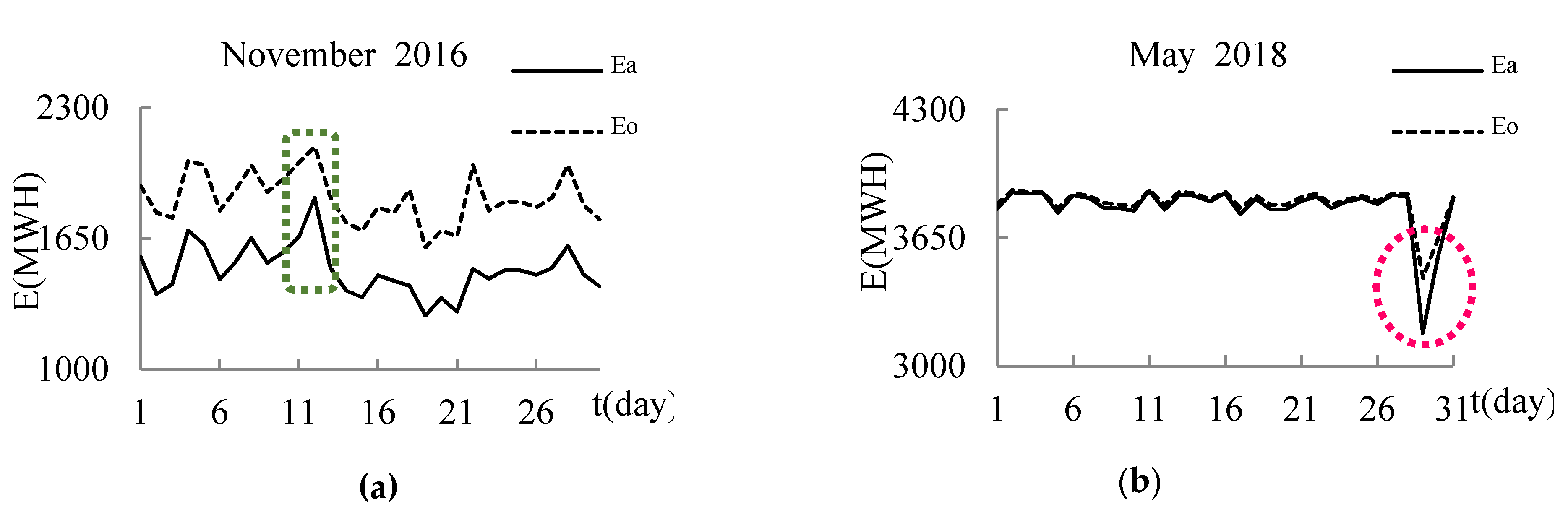
As shown in Figure 4, the optimal power generation curve was higher than actual power generation curve in November, 2016. This means that the power generation was optimal and the cost was economical as it could be run effectively with less water consumption. The highest power generation was reached on 12 November, as shown in green dotted rectangular in Figure 4a, when optimal power generation was 2105 MWH whereas the actual power generation was 1850.4 MWH and the efficiency was 13.7 percent, the lowest among in this month. This means the power generation is optimal when the optimal value is larger than actual value whereas the efficiency is minimum. In May 2018, as shown in Figure 4b, the optimal and actual power generation curves overlap each other between 3800 MWH and 3900 MWH and drop sharply to 3488.3 MWH in 29 May, as shown in the pink dotted circle, therefore, when the optimized power generation was larger than the actual operating power generation result, and the optimization efficiency was low. In contrast, the actual and optimal power generation was the same and there was almost no gap within the two curves in most days.

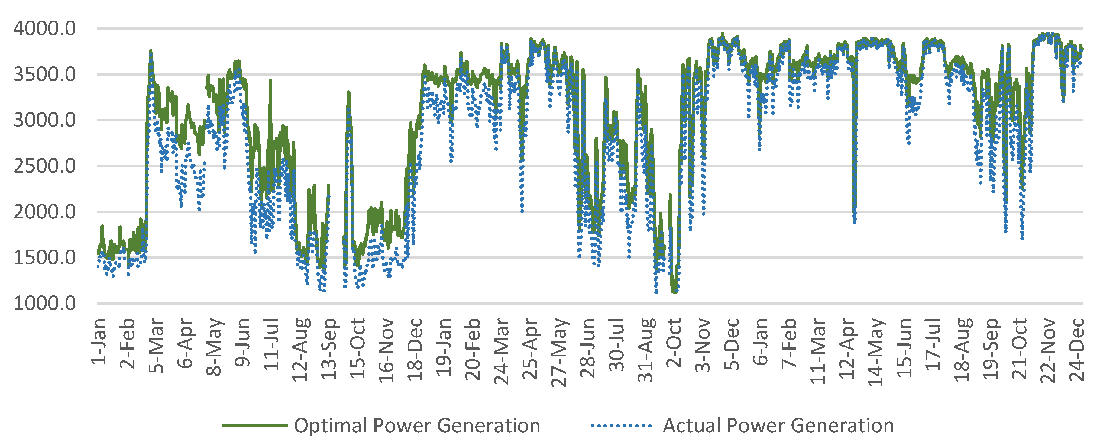
From the data shown in Figure 5, the generation curves oscillate inconstantly due to the load demand changes that caused the load distribution units instability. In actual power generation, the emergency start up and shut down raises the water consumption level. In water consumption, the optimal solution saves 1.36% more than actual operation [23] whereas it saves up to 2% for the same turbine types [14]. In this paper, the optimal water consumption saved up to 10% more than actual operation and the load generation was higher than actual operation in optimal solution in every time period from 2016 to 2018. In contract, the results give the advantageous optimization operation which satisfies the cost benefit effects.

4. Conclusions

By optimizing the optimal operation of hydropower station from the 2016 to 2018 daily and monthly data of Baluchaung II hydropower station by programming, the optimized power generation flow of the hydropower station could be obtained. Dynamic programming was used for optimal generation with minimum generation flow for saving water especially in the drought season. In power generation flow, the best optimization result was obtained when the optimization efficiency reached 17.75% when water quantity was small whereas in power generation, the optimization efficiency is 24.16% for better optimal operation. In the unit allocation, based on the characteristics of the fitted NQ curve, we found that maximizing the output of the unit could optimize the efficiency of the power generation flow and also noticed that the optimization effect of the power generation flow was poor due to the incoming water volume being large. However, in this simulation, the results showed that total water consumption of optimal solution could save a larger amount of water consumption than actual operation and monthly scale generation flow results for optimal solution were lower than the actual operation data in every month during three years. Whereas in power generation, the optimization result was higher than the actual result in each month within the three years. Due to the point in contrast, the operation was optimal within three years. The key limitation of this paper, is that it does not consider some other constraints in the reckoning process and the future scholar could take into account start up/shut down and power plant equipment constraints in the case of optimal operation.

References

- Ogayar, B.; Vidal, P.G.; Hernandez, J.C. Analysis of the cost for the refurbishment of small hydropower plants. Renew. Energy 2009, 34, 2501–2509. [Google Scholar] [CrossRef]
- Konga, J.; Skjelbreda, H.I.; Fossob, O.B. An overview on formulations and optimization methods for the unit-based short-term hydro scheduling problem. Electr. Power Energy Syst. 2020, 178, 106027–106041. [Google Scholar] [CrossRef]
- Parvez, B.L.I.; Shen, J.; Khan, M.; Cheng, C. Modeling and Solution Techniques Used for Hydro Generation Scheduling. Water 2019, 11, 1392. [Google Scholar] [CrossRef] [Green Version]
- Marchand, A.; Gendreau, M.; Blais, M.; Guidi, J. Optimized Operating Rules for Short-Term Hydropower Planning in a Stochastic Environment; Springer: Berlin/Heidelberg, Germany, 2019. [Google Scholar]
- Osório, G.J.; Matias, J.C.O.; Catalão, J.P.S. A Review of Short-Term Hydro Scheduling Tools. In Proceedings of the 48th International Universities Power Engineering Conference, Dublin, Ireland, 2–5 September 2013. [Google Scholar]
- Liu, P.; Nguyen, T.; Cai, X.; Jiang, X. Finding Multiple Optimal Solutions to Optimal Load Distribution Problem in Hydropower Plant. Energies 2012, 5, 1413–1432. [Google Scholar] [CrossRef]
- Hans, I.S.; Jiehong, K.; Olav, B.F. Dynamic incorporation of nonlinearity into MILP formulation for short-term hydro scheduling. Electr. Power Energy Syst. 2020, 116, 105530–105547. [Google Scholar]
- Yuan, Y. An Improved PSO approach to Short-term Economic Dispatch of Cascaded Hydropower Plants. Kybernetes 2010, 8, 1359–1365. [Google Scholar] [CrossRef]
- Moreno, S.R.; Kaviski, E. Daily Scheduling of small hydro power plants dispatch with modified particles swarm optimization. Scielo Anal. J. 2012, 35, 25–37. [Google Scholar] [CrossRef] [Green Version]
- Xie, W.; Ji, C.-M.; Yang, Z.; Zhang, X. Short-term power generation scheduling rules for cascade hydropower stations based on hybrid algorithm. Water Sci. Eng. J. 2012, 5, 46–58. [Google Scholar]
- Liao, S.; Liu, J.; Liu, B.; Cheng, C.; Zhou, L.; Wu, H. Multicore Parallel Dynamic Programming Algorithm for Short-Term Hydro-Unit Load Dispatching of Huge Hydropower Stations Serving Multiple Power Grids. Water Resour. Manag. 2020, 34, 359–376. [Google Scholar] [CrossRef]
- Ji, C.; Xie, W.; Yang, Z.; Zhang, X.; Zhu, X. Study of the scheduling rules of short-term power generation dispatching for single hydropower station. In Proceedings of the International Conference on Industrial Control and Electronics Engineering, Xian, China, 23–25 August 2012. [Google Scholar]
- Zou, Q.; Li, A.; He, X.; Wang, X. Optimal Operation of Cascade Hydropower Stations Based on Chaos Cultural Sine Cosine Algorithm. In Proceedings of the Asia Conference on Power and Electrical Engineering, Kitakyushu, Japan, 22–24 March 2018. [Google Scholar]
- Chu, Q.; Li, W.; Sun, C. Research of Economic Operation in Hydropower Station Based on Recursive Optimization. Adv. Mater. Res. 2012, 524–527, 2905–2910. [Google Scholar] [CrossRef]
- Zhang, Y.; Liu, Y.; Wu, Y.; Ji, C.; Ma, Q. Short-Term Optimal Operation of Cascade Reservoirs Considering Dynamic Water Flow Hysteresis. Water 2019, 11, 2098. [Google Scholar] [CrossRef] [Green Version]
- Olawale, O.E.A. Optimizing Hydroelectric Power Generation: The Case of Shiroro Dam. In Proceedings of the World Congress on Engineering, Landon, UK, 5–7 July 2017. [Google Scholar]
- Getachew, E.; Mamo, M.M.; Carlos, J.; Hurtado, C.; Franca, M.J. Optimization of Run-of-River Hydropower Plant Capacity. Int. Water Power Dam Constr. 2018. Available online: https://www.waterpowermagazine.com. (accessed on 3 August 2018).
- Liao, S.; Zhao, H.; Li, G.; Liu, B. Short-Term Load Dispatching Method for a Diversion Hydropower Plant with Multiple Turbines in One Tunnel Using a Two-Stage Model. Energies 2019, 2019, 1476. [Google Scholar] [CrossRef] [Green Version]
- Guedes, L.S.M.; Maia, P.M.; Lisboa, A.C.; Vieira, D.A.G.; Saldanha, R.R. A unit commitment algorithm and a compact MILP model for short-term hydro-power generation scheduling. IEEE Trans. Power Syst. 2017, 32, 3381–3390. [Google Scholar] [CrossRef]
- Hering, P.; Mosna, J.; Janecek, E.; David, H. Optimal scheduling of a pumped-storage hydro power plant operation. In Proceedings of the 13th International Conference on Environment and Electrical Engineering, Wroclaw, Poland, 1–3 November 2013. [Google Scholar]
- Ai, X.; Chen, S. Short-term Operation Method and Hydraulic Calculation of Three Gorges Cascade. In Proceedings of the 2010 Asia-Pacific Power and Energy Engineering Conference, Chengdu, China, 28–31 March 2010. [Google Scholar]
- Chen, S.L. Reservoir Operation and Operation of Hydropower Station; China Electric Power Press: Beijing, China, 2008. [Google Scholar]
- Peng, L.; Jian, Z.; Chao, Q.; Qiao, M. Short-term hydro generation scheduling of Xiluodu and Xiangjiaba cascade hydropower stations using improved binary-real coded bee colony optimization algorithm. Energy Convers. Manag. 2015, 91, 19–31. [Google Scholar]
Figure 1.
Waterway System of Baluchaung II hydropower station.
Figure 2.
Unit dynamic characteristic NQ curve.
Figure 3.
Actual and optimal power generation flow chart for November and January 2016.
Figure 4.
Optimal and actual power generation chart of January 2016 and February 2017.3.3. Power Generation Optimization.
Figure 5.
Optimal and power generation chart for 2016–2018.