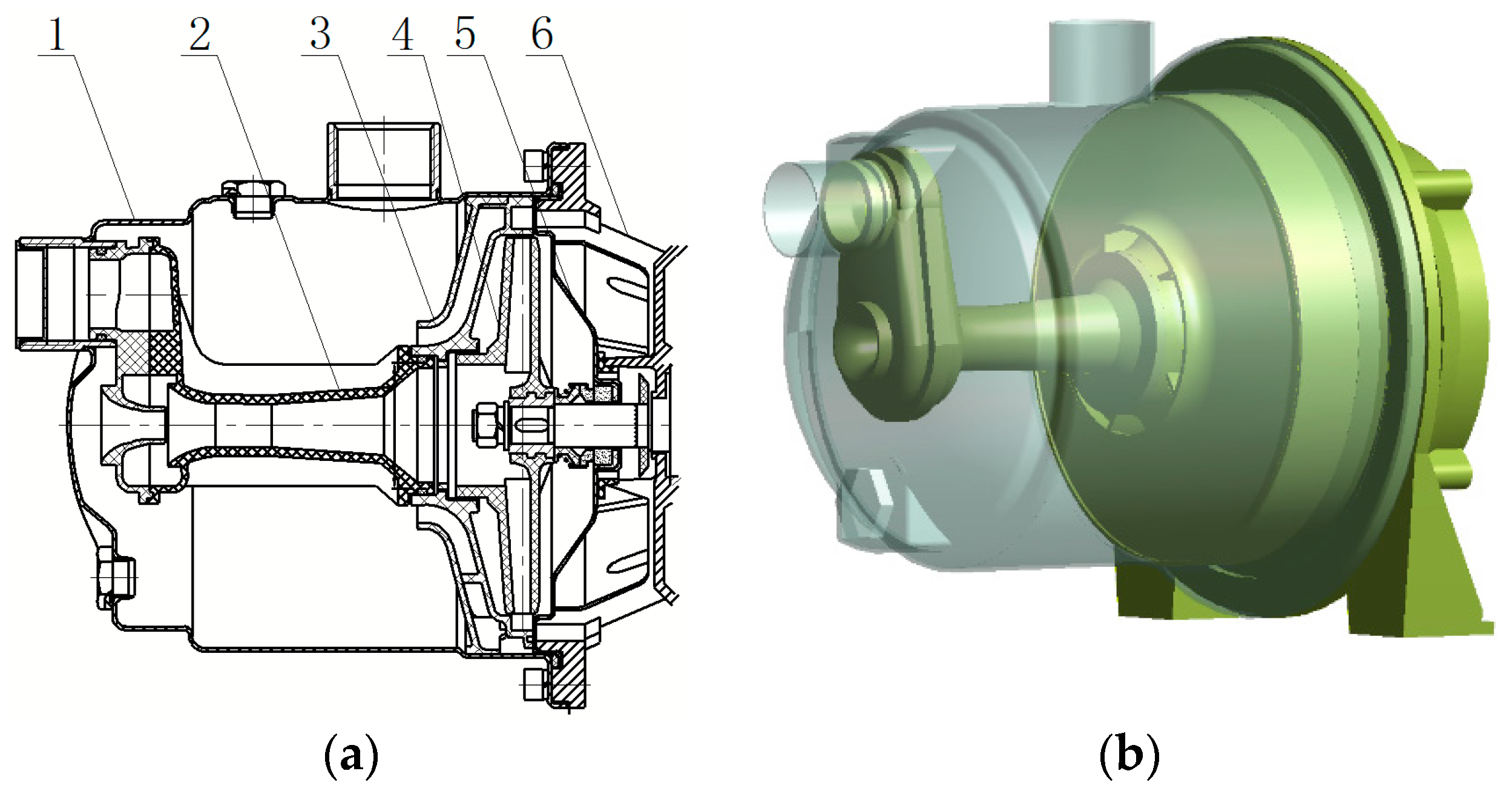
Figure 1.
Structural diagrams of the model pump. (a) Two-dimensional structure diagram; (b) three-dimensional structure diagram. 1: Pump body; 2: Jet; 3: Guide vane; 4: Impeller; 5: Pump cover; 6: Bracket.
Figure 1.
Structural diagrams of the model pump. (a) Two-dimensional structure diagram; (b) three-dimensional structure diagram. 1: Pump body; 2: Jet; 3: Guide vane; 4: Impeller; 5: Pump cover; 6: Bracket.
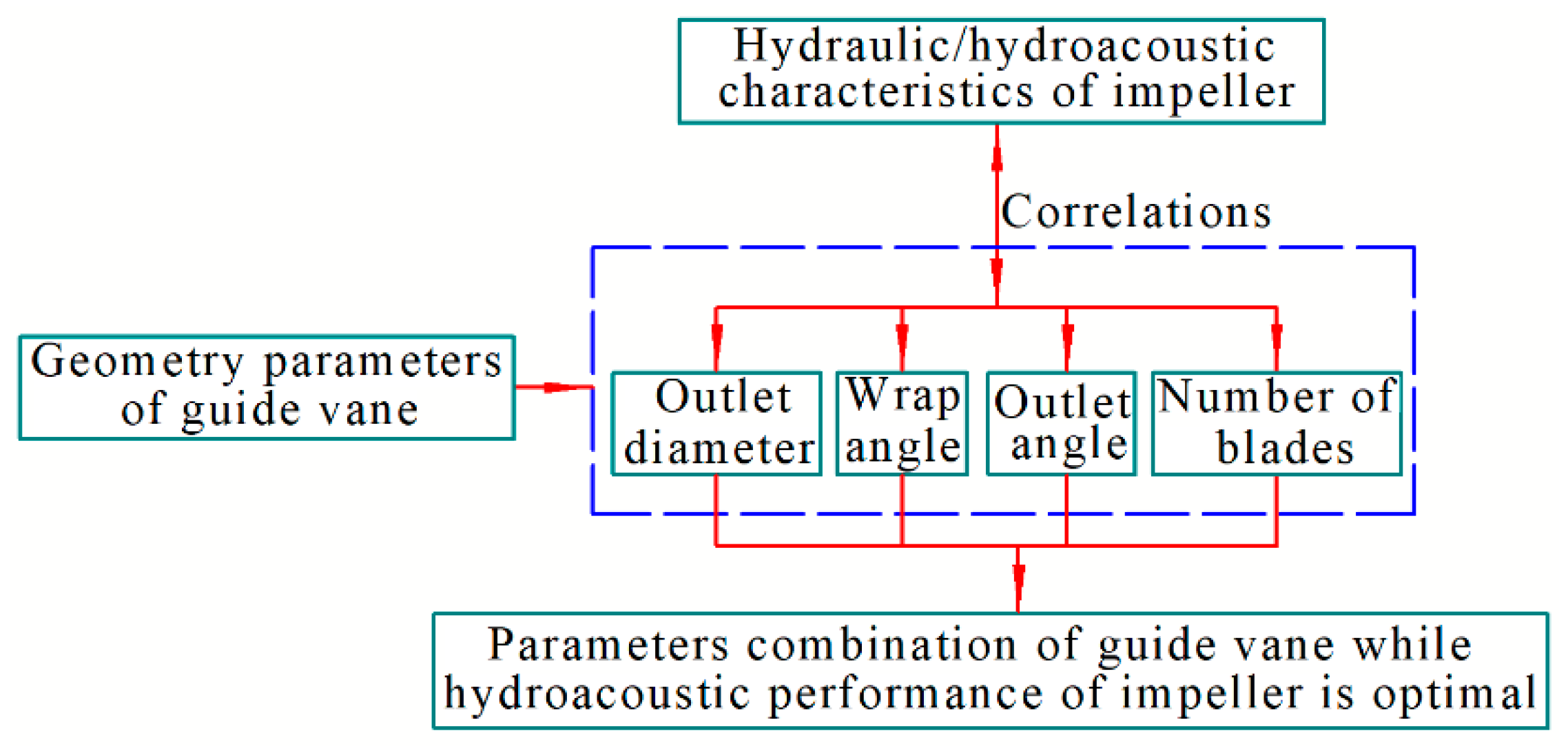
Figure 2.
Research routes followed in this study.
Figure 2.
Research routes followed in this study.
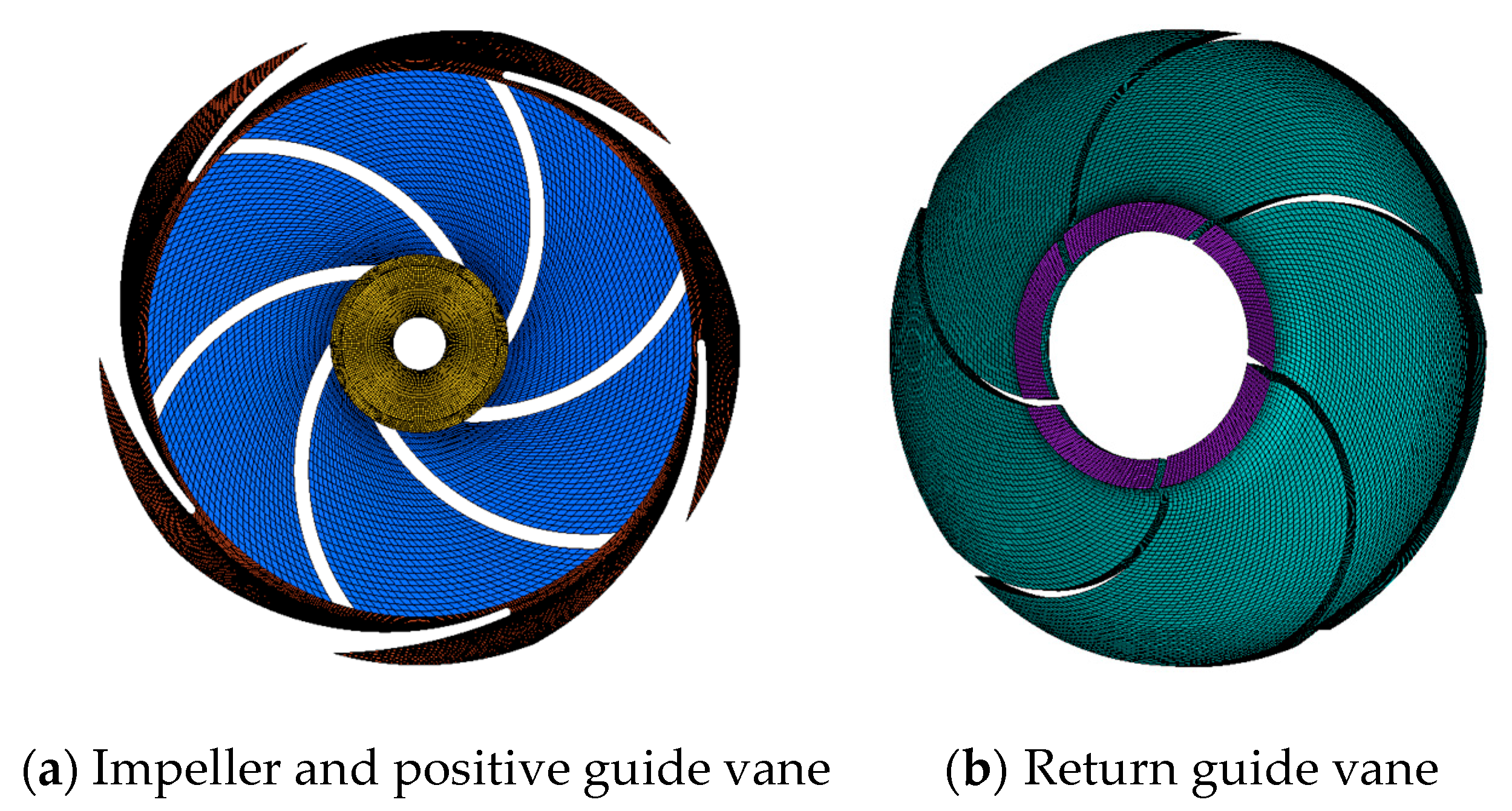
Figure 3.
Grid diagram of the impeller and guide vane of the model jet centrifugal pumps (JCP).
Figure 3.
Grid diagram of the impeller and guide vane of the model jet centrifugal pumps (JCP).
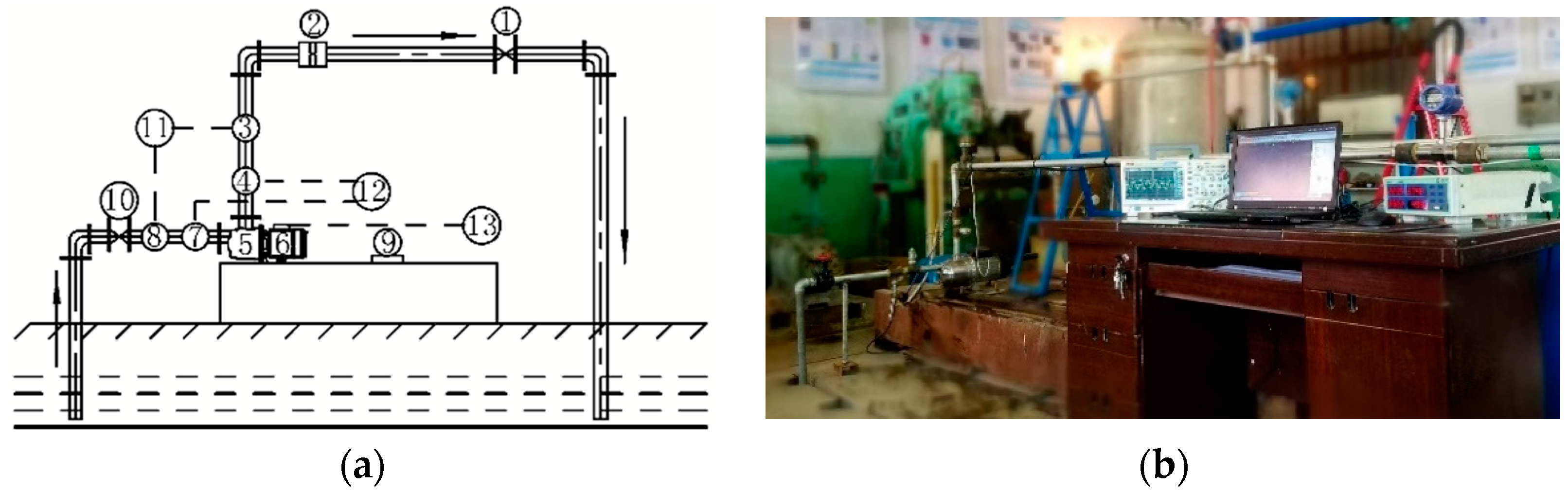
Figure 4.
Test system. (a) Schematic diagram of the test system structure; (b) test site. 1: Valve at pump outlet; 2: Flowmeter; 3: Pressure sensor at pump outlet; 4: Hydrophone at pump outlet; 5: Model pump; 6: Electric motor; 7: Hydrophone at pump inlet; 8: Pressure sensor at pump inlet; 9: Tachometer; 10: Valve at pump inlet; 11: Computer; 12: Oscilloscopes; 13: Measuring instrument of electric power.
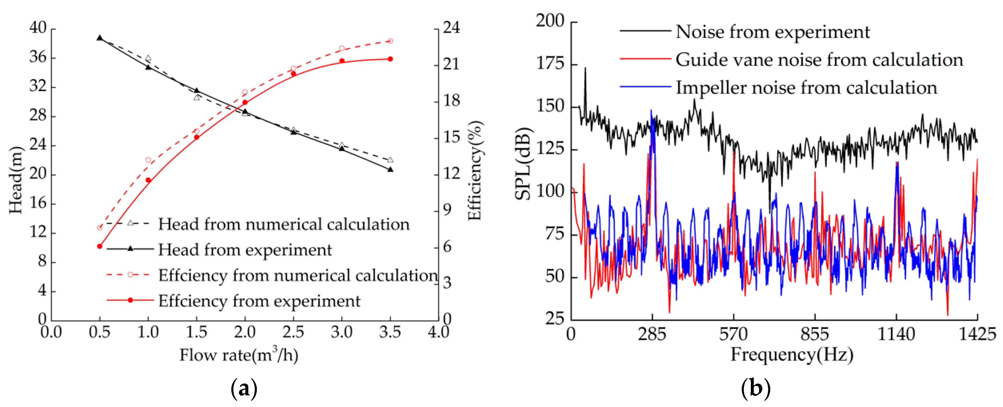
Figure 5.
Comparison of performances between the experiment and numerical calculation. (a) Comparison of hydraulic performance; (b) comparison of frequency response curves of the sound pressure level.
Figure 5.
Comparison of performances between the experiment and numerical calculation. (a) Comparison of hydraulic performance; (b) comparison of frequency response curves of the sound pressure level.
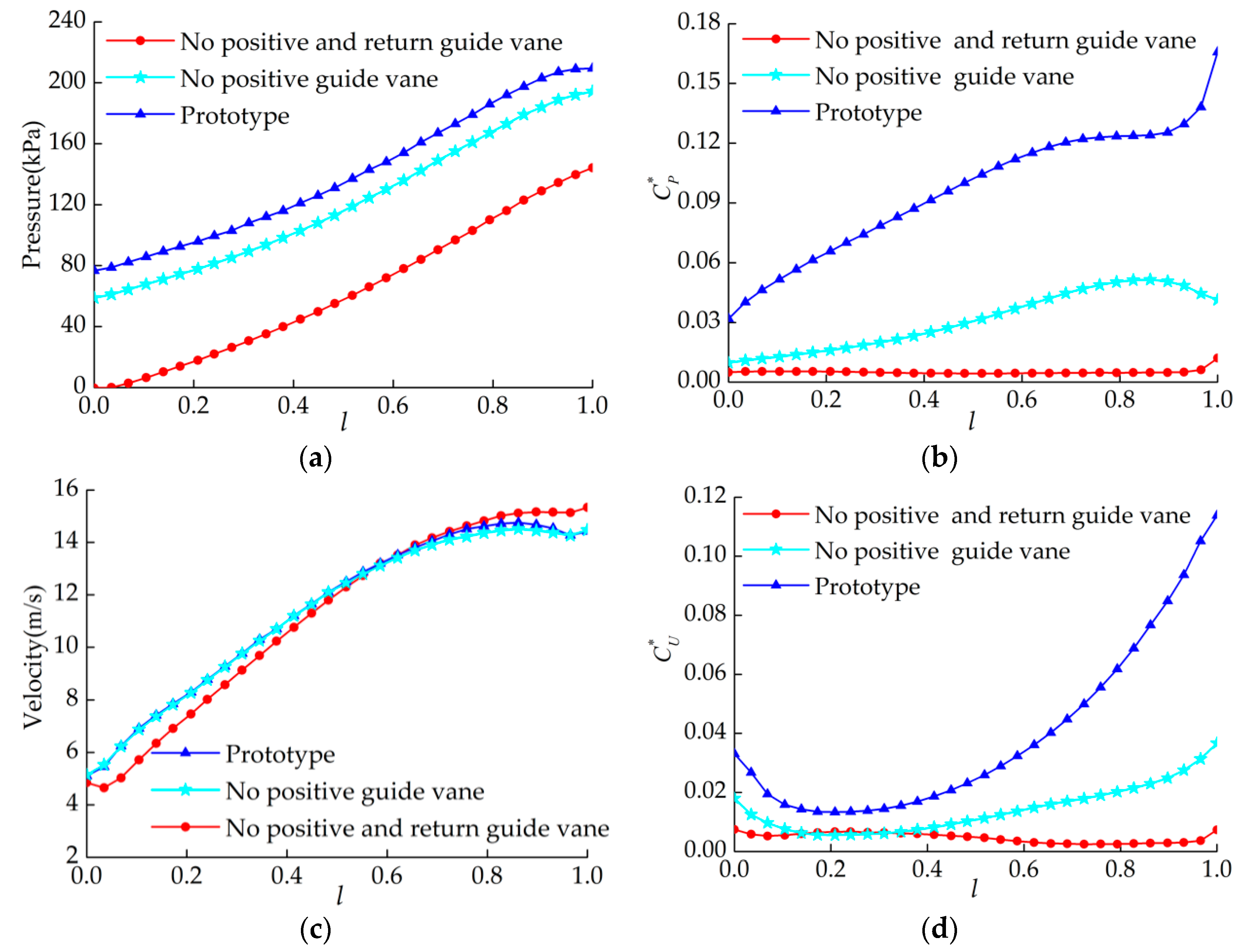
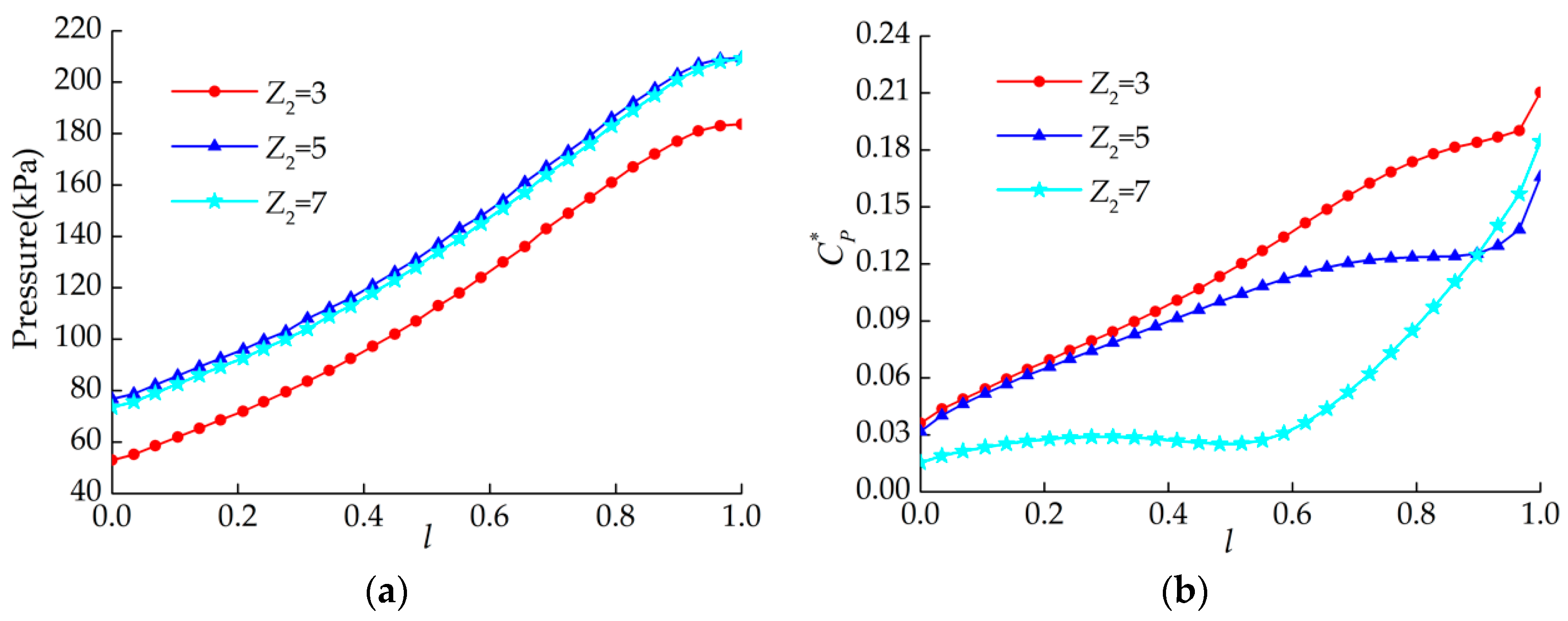
Figure 6.
The time-average and fluctuation intensity curves of pressure and velocity on the blade surface of the impeller with different blade numbers of the guide vane. (a) The curves of the pressure time-average; (b) the curves of pressure fluctuation intensity; (c) the curves of the velocity time-average; (d) the curves of velocity fluctuation intensity.
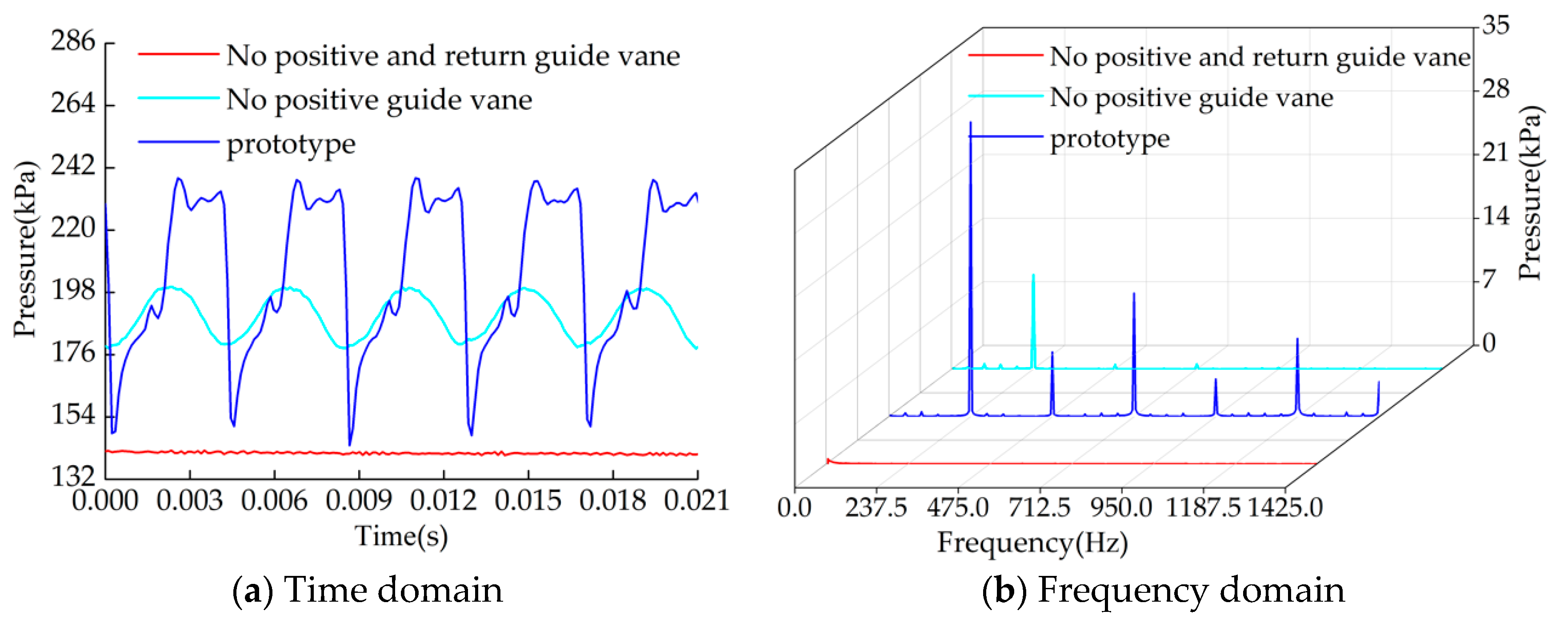
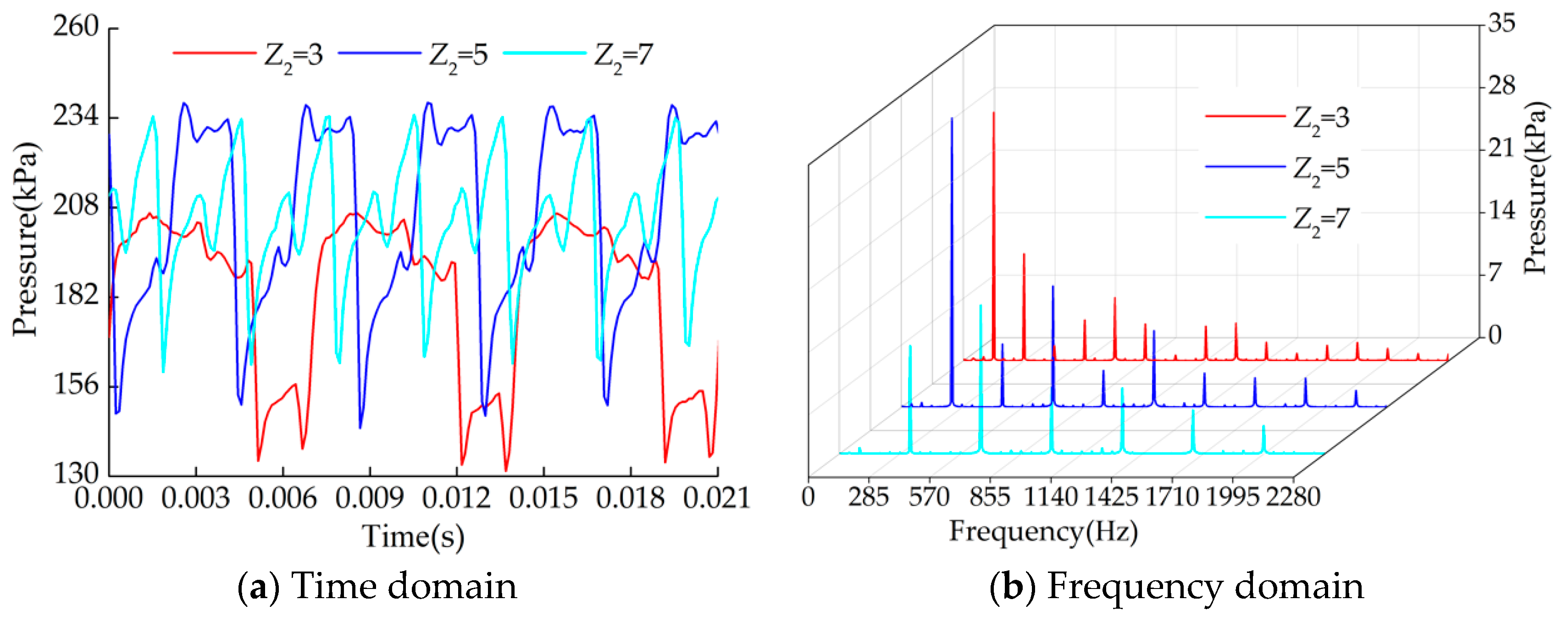
Figure 7.
Time and frequency response curves of pressure inside the impeller for different blade numbers of the guide vane.
Figure 7.
Time and frequency response curves of pressure inside the impeller for different blade numbers of the guide vane.
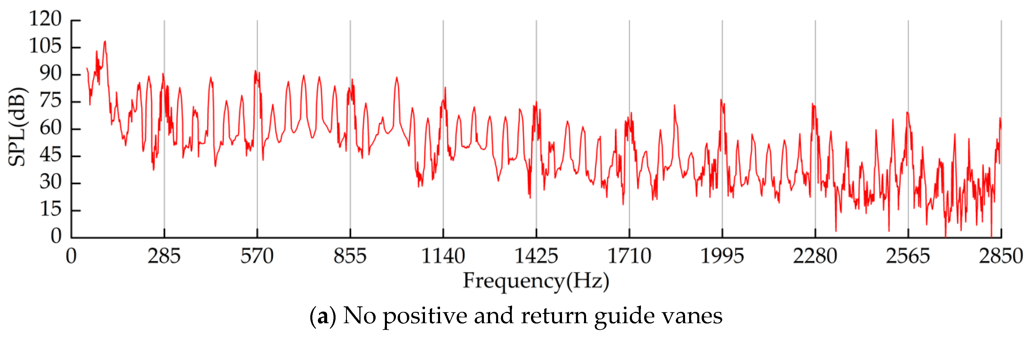
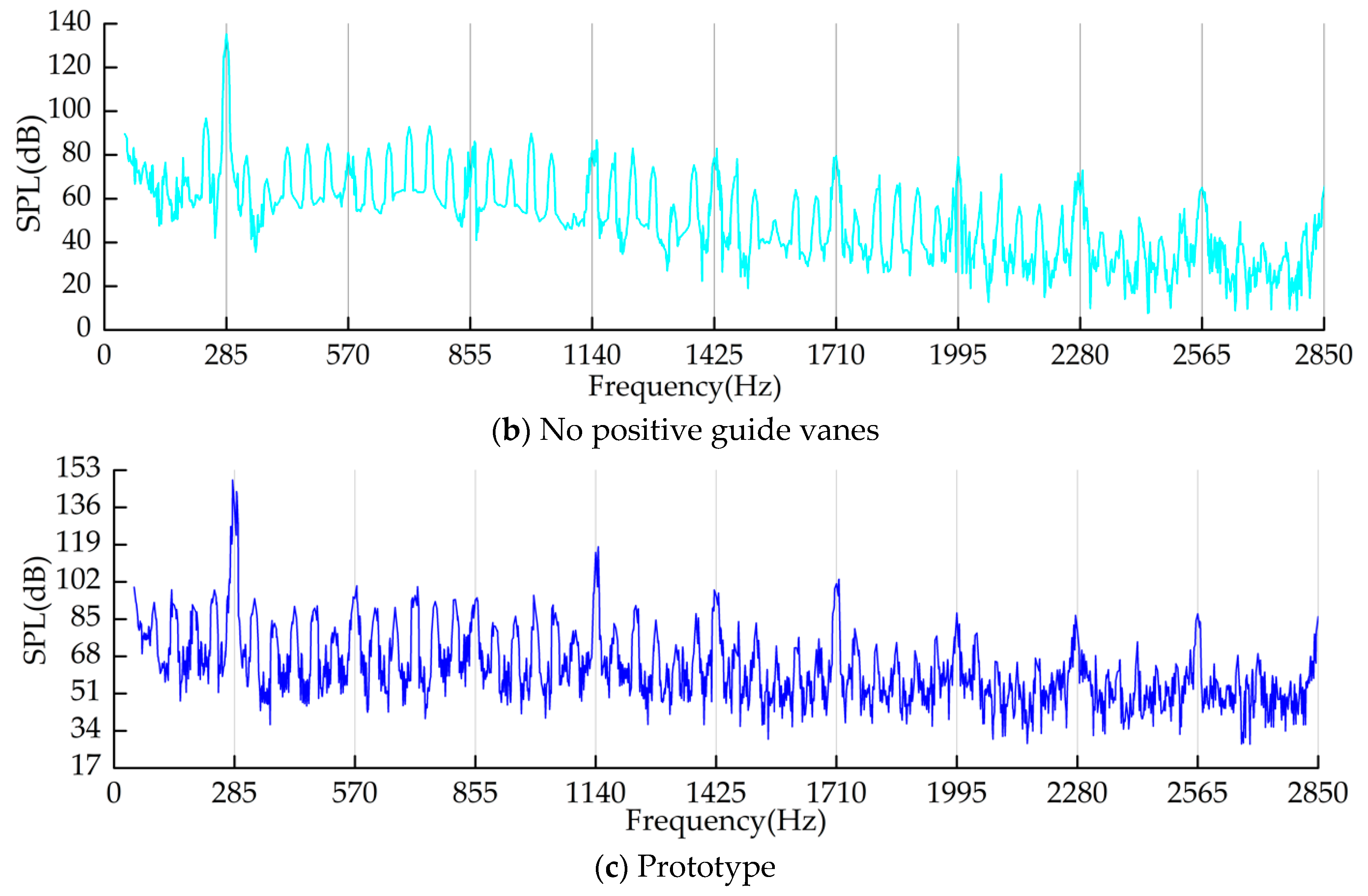
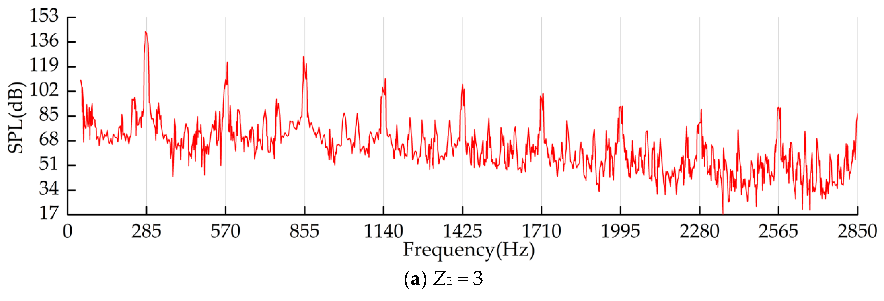
Figure 8.
Frequency response curves of the hydroacoustic sound pressure level (SPL) of the impeller with different blade numbers of the guide vane.
Figure 8.
Frequency response curves of the hydroacoustic sound pressure level (SPL) of the impeller with different blade numbers of the guide vane.
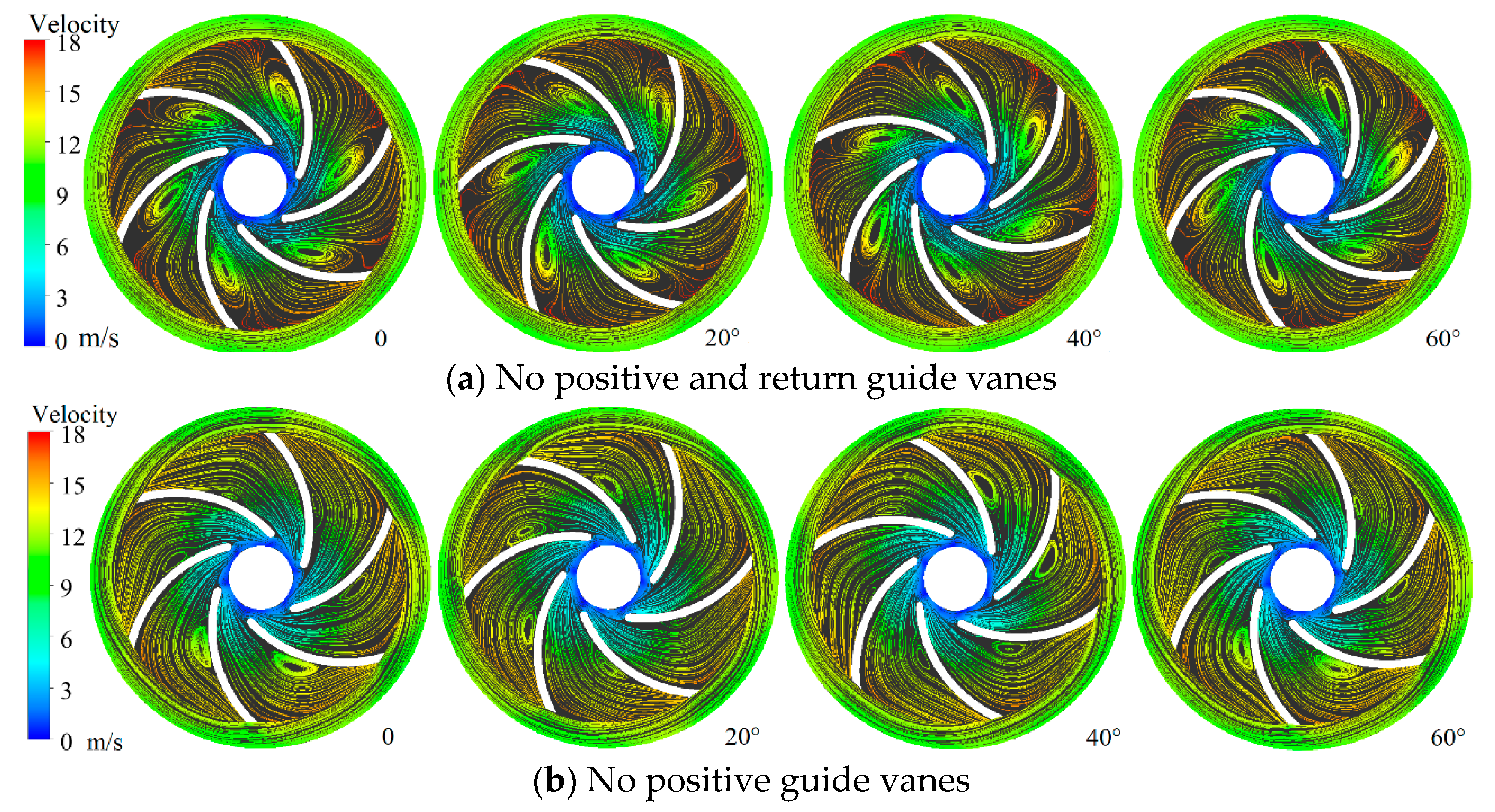
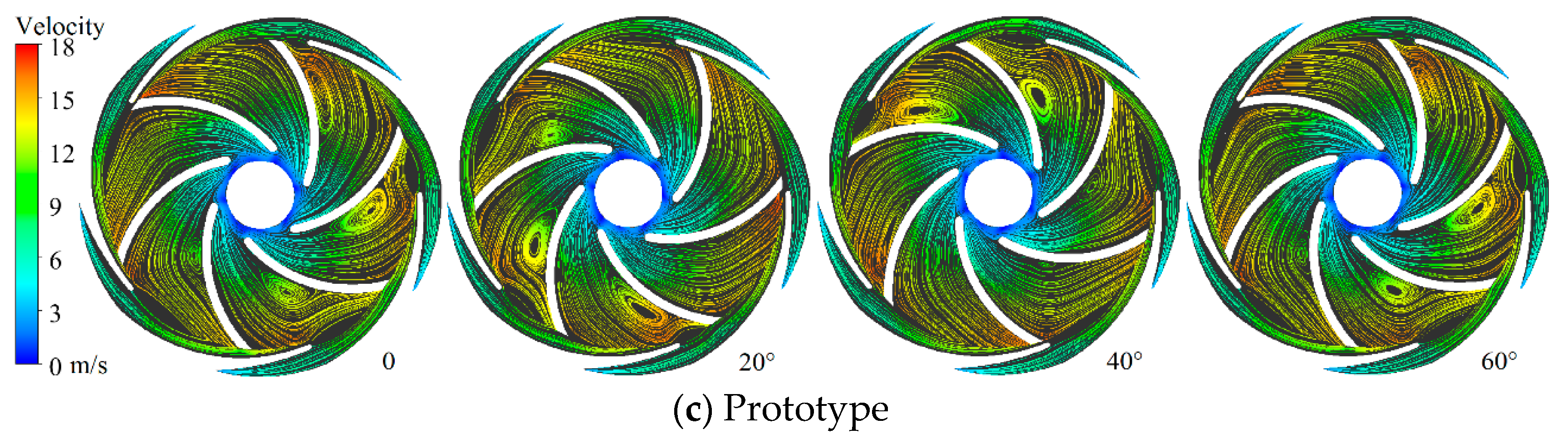
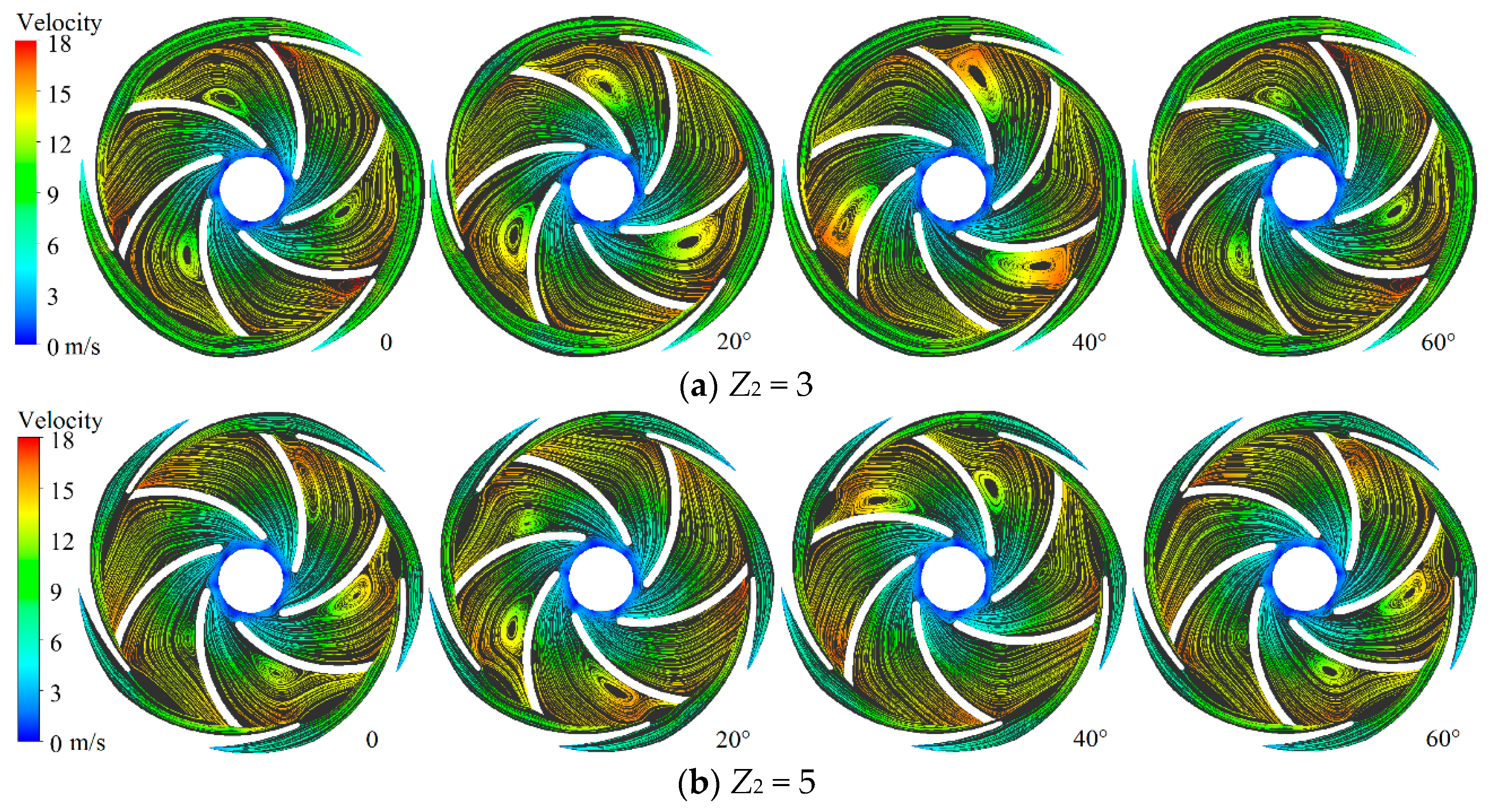
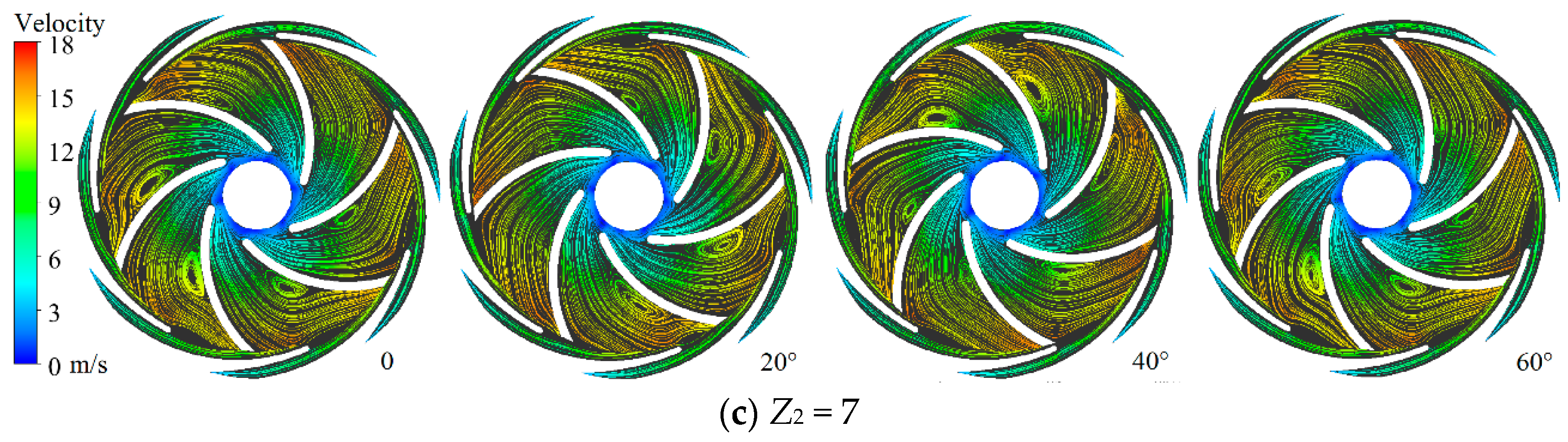
Figure 9.
Evolution processes of the transient flow field inside the impeller and guide vane with different blade numbers of the guide vane.
Figure 9.
Evolution processes of the transient flow field inside the impeller and guide vane with different blade numbers of the guide vane.
Figure 10.
The time-average and the fluctuation intensity curves of pressure and velocity on the blade surface of the impeller with different numbers of guide vanes. (a) The curves of the pressure time-average; (b) the curves of pressure fluctuation intensity; (c) the curves of the velocity time-average; (d) the curves of velocity fluctuation intensity.
Figure 11.
Time and frequency response curves of pressure inside the impeller with different numbers of guide vanes.
Figure 11.
Time and frequency response curves of pressure inside the impeller with different numbers of guide vanes.
Figure 12.
Frequency response curves of the hydroacoustic SPL inside the impeller with different numbers of guide vanes.
Figure 12.
Frequency response curves of the hydroacoustic SPL inside the impeller with different numbers of guide vanes.
Figure 13.
Evolution processes of the transient flow field inside the impeller and guide vane with the different blade numbers of the guide vane.
Figure 13.
Evolution processes of the transient flow field inside the impeller and guide vane with the different blade numbers of the guide vane.
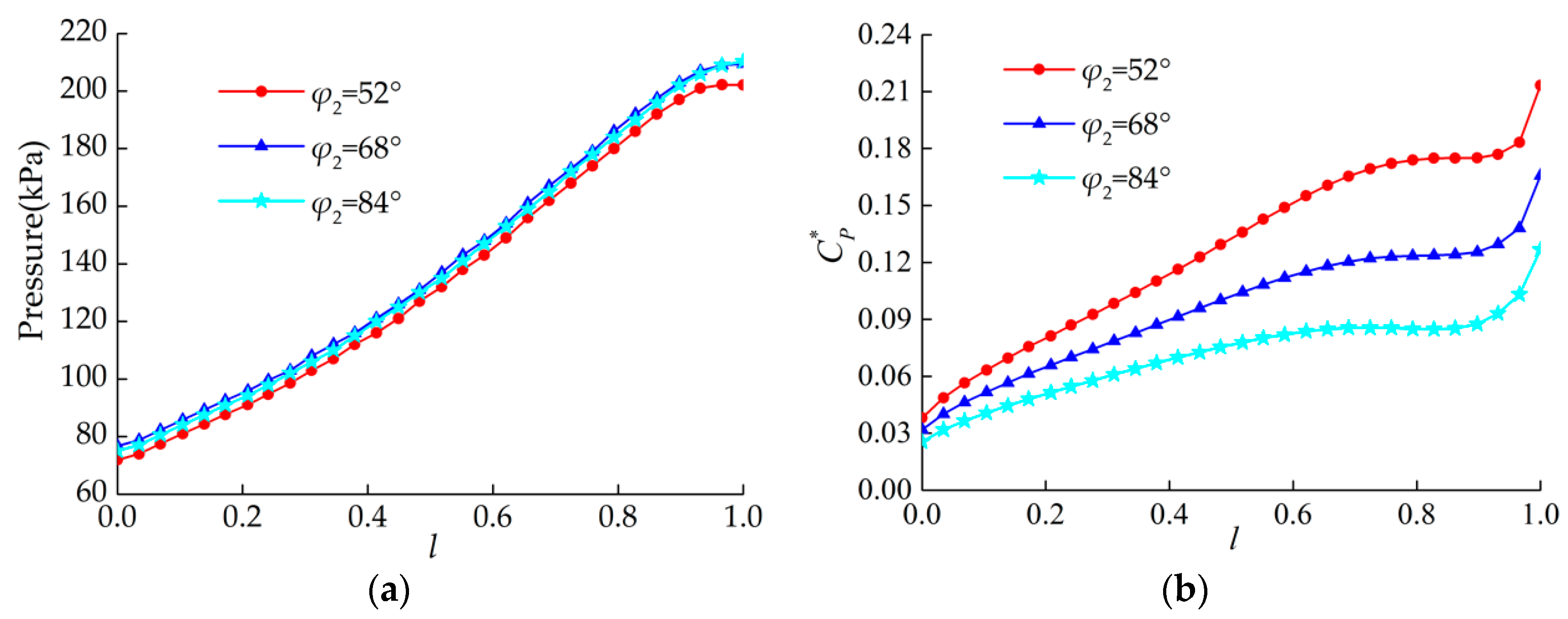
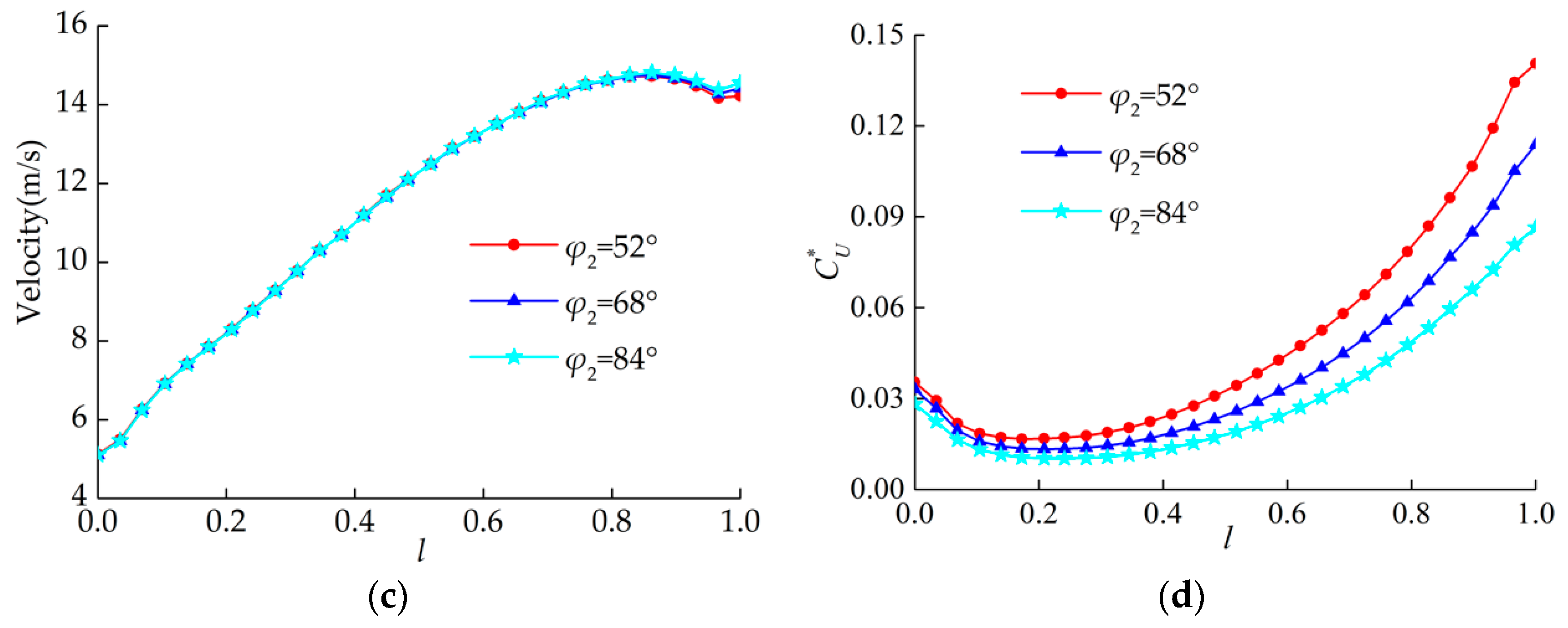
Figure 14.
The time-average and the fluctuation intensity curves of pressure and velocity on the blade surface of the impeller with different wrap angles of the positive guide vane. (a) The curves of the pressure time-average; (b) the curves of pressure fluctuation intensity; (c) the curves of the velocity time-average; (d) the curves of velocity fluctuation intensity.
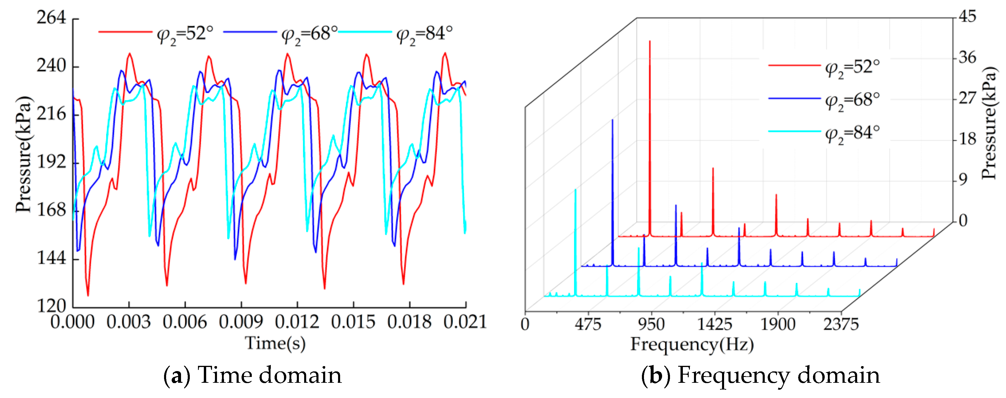
Figure 15.
Frequency response curves of pressure inside the impeller with different wrap angles of the positive guide vane.
Figure 15.
Frequency response curves of pressure inside the impeller with different wrap angles of the positive guide vane.
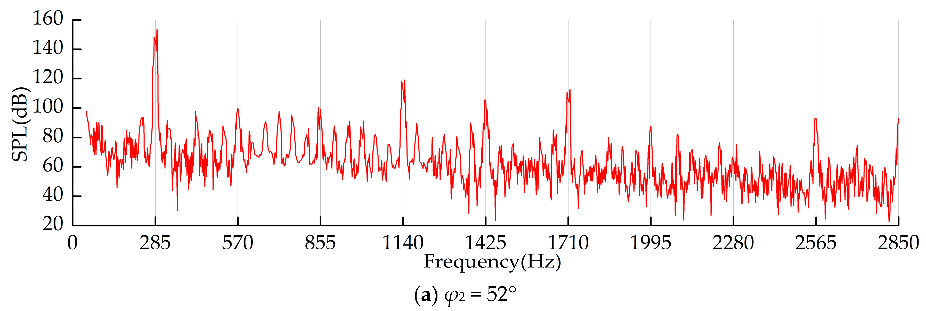
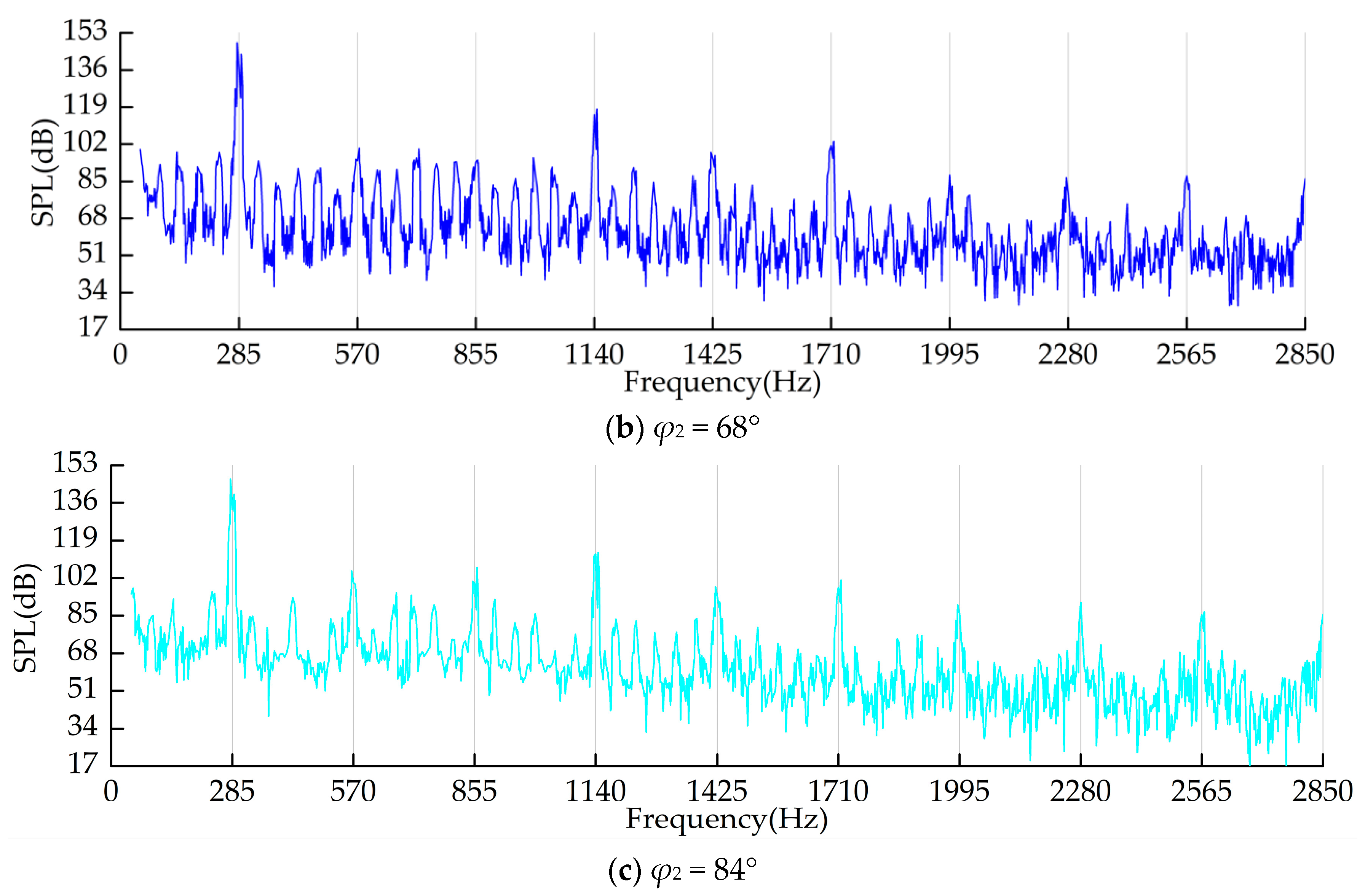
Figure 16.
Frequency response curves of the hydroacoustic SPL inside the impeller with different wrap angles of the positive guide vane.
Figure 16.
Frequency response curves of the hydroacoustic SPL inside the impeller with different wrap angles of the positive guide vane.
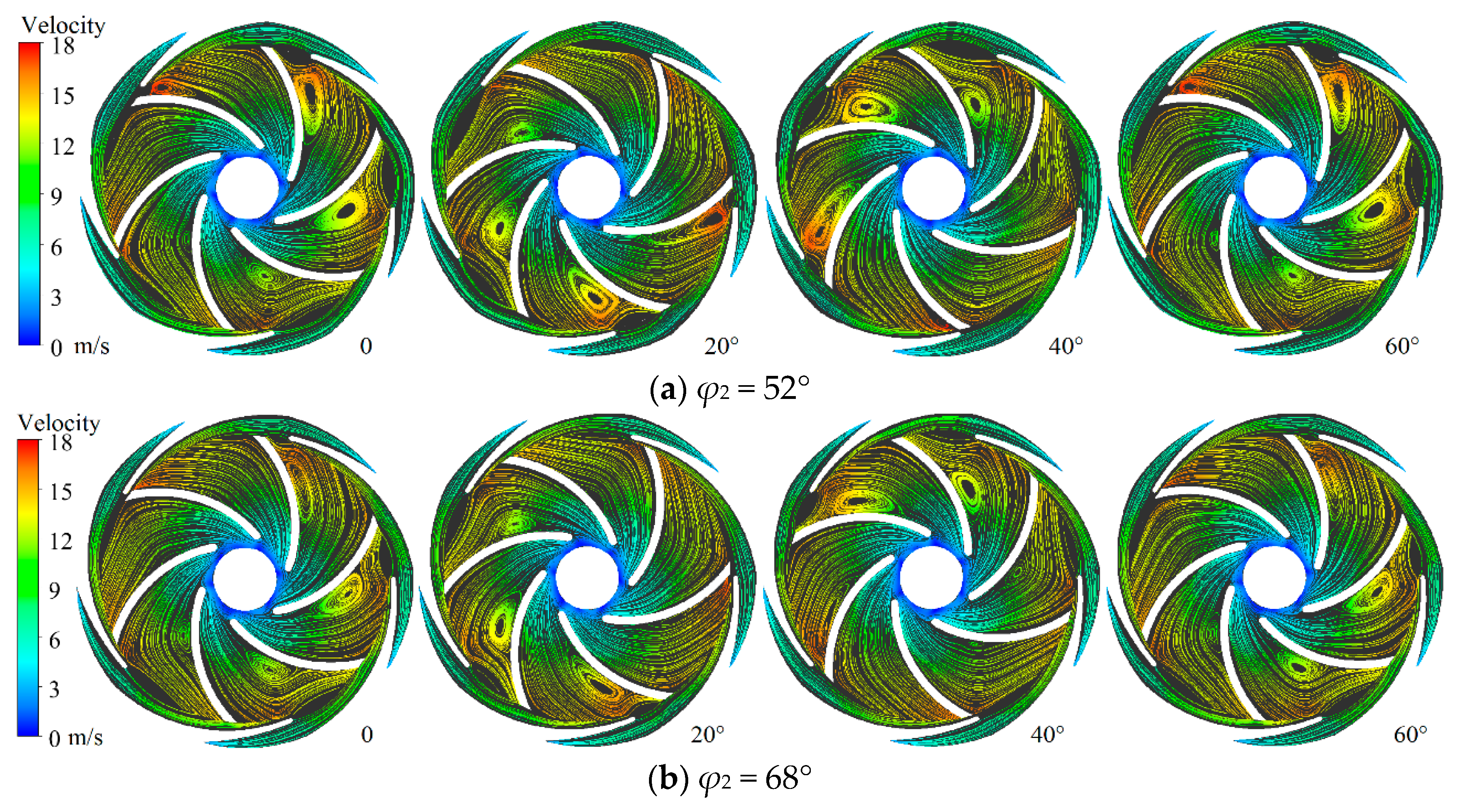
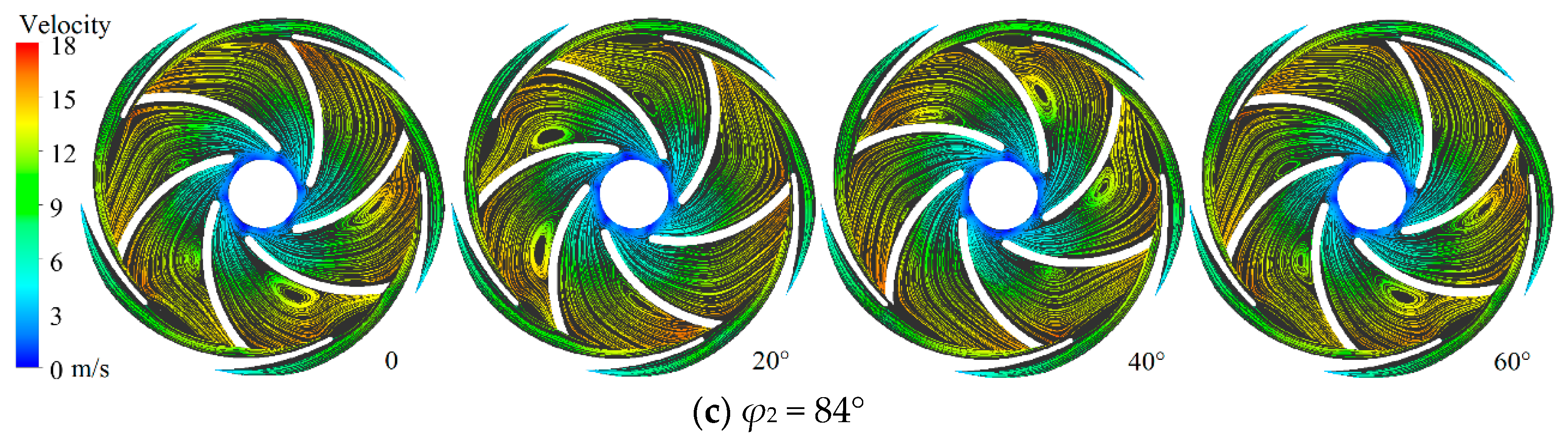
Figure 17.
Evolution processes of the transient flow field inside the impeller and guide vane with different wrap angles of the positive guide vane.
Figure 17.
Evolution processes of the transient flow field inside the impeller and guide vane with different wrap angles of the positive guide vane.
Figure 18.
The time-average and the fluctuation intensity curves of pressure and velocity on the blade surface of the impeller with different wrap angles of the positive guide vane. (a) The curves of the pressure time-average; (b) the curves of pressure fluctuation intensity; (c) the curves of the velocity time-average; (d) the curves of velocity fluctuation intensity.
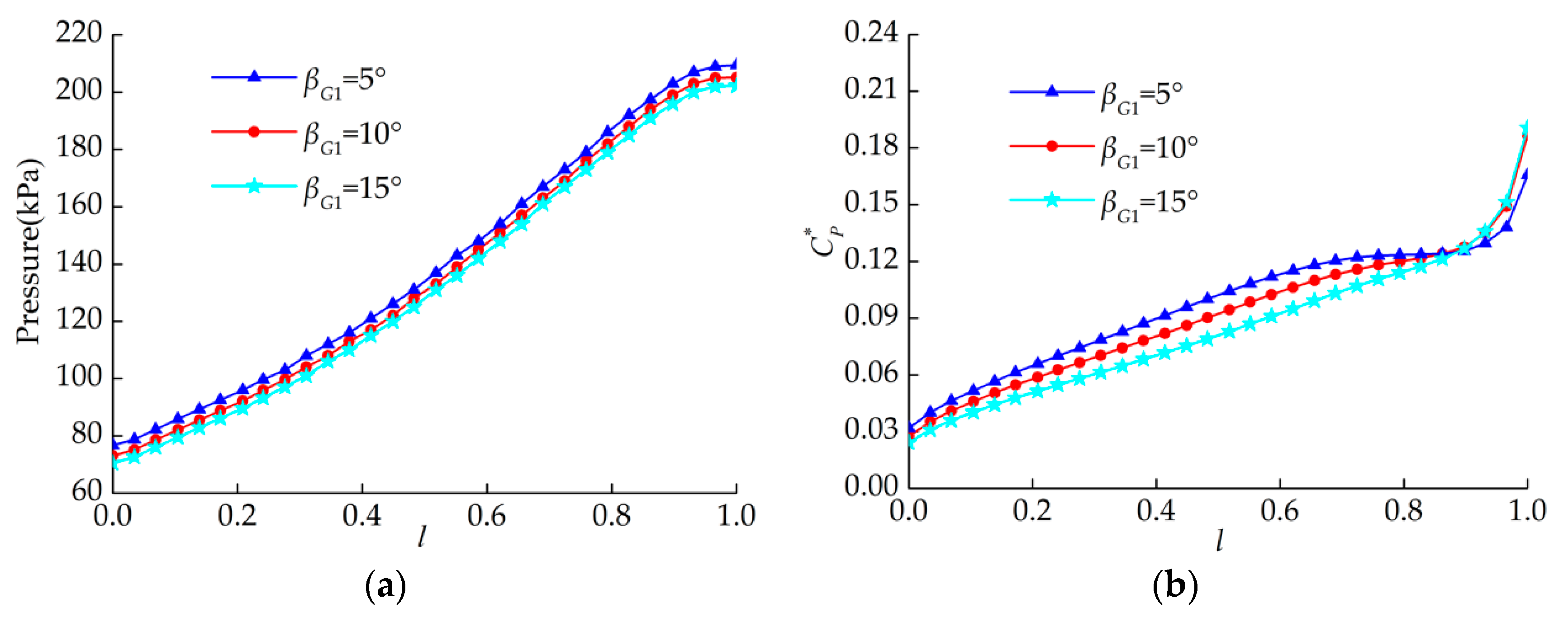
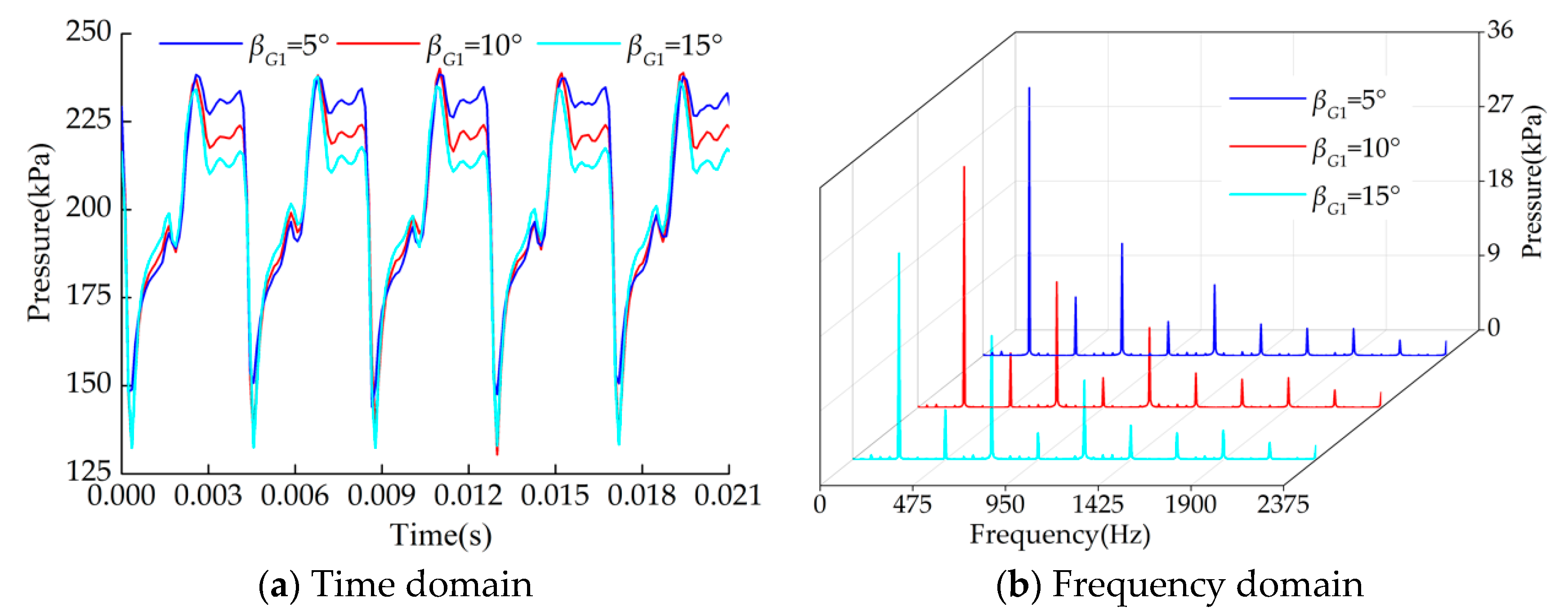
Figure 19.
Time and frequency response curves of pressure inside the impeller with different inlet angles of the positive guide vane.
Figure 19.
Time and frequency response curves of pressure inside the impeller with different inlet angles of the positive guide vane.
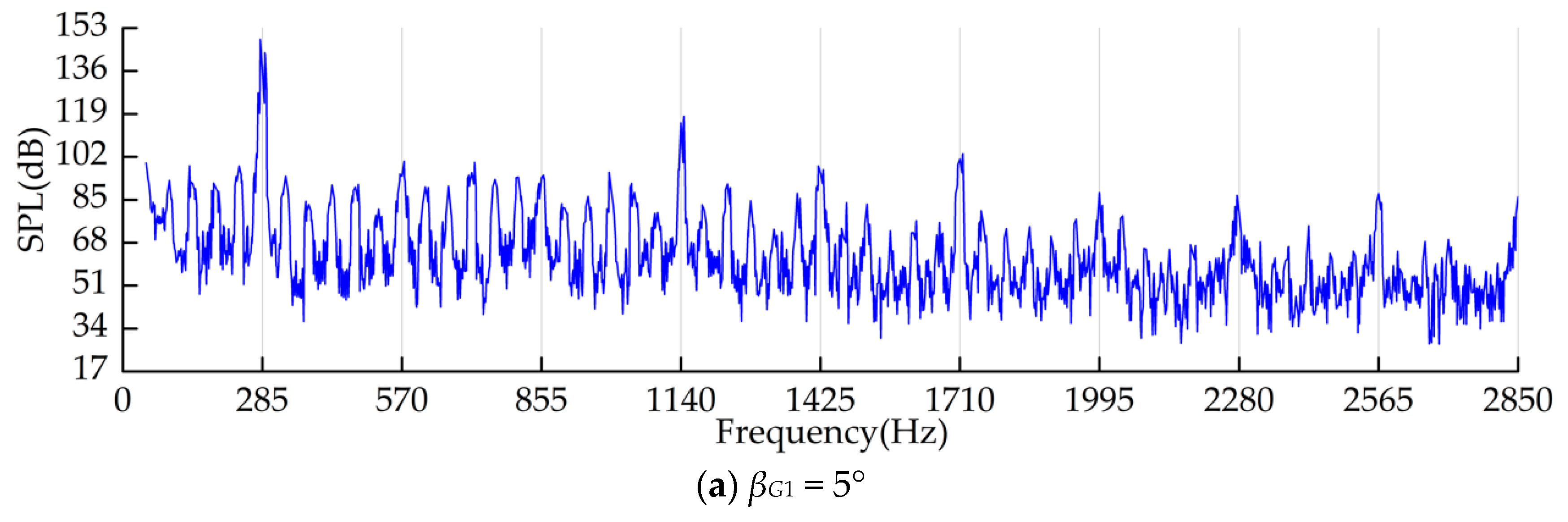
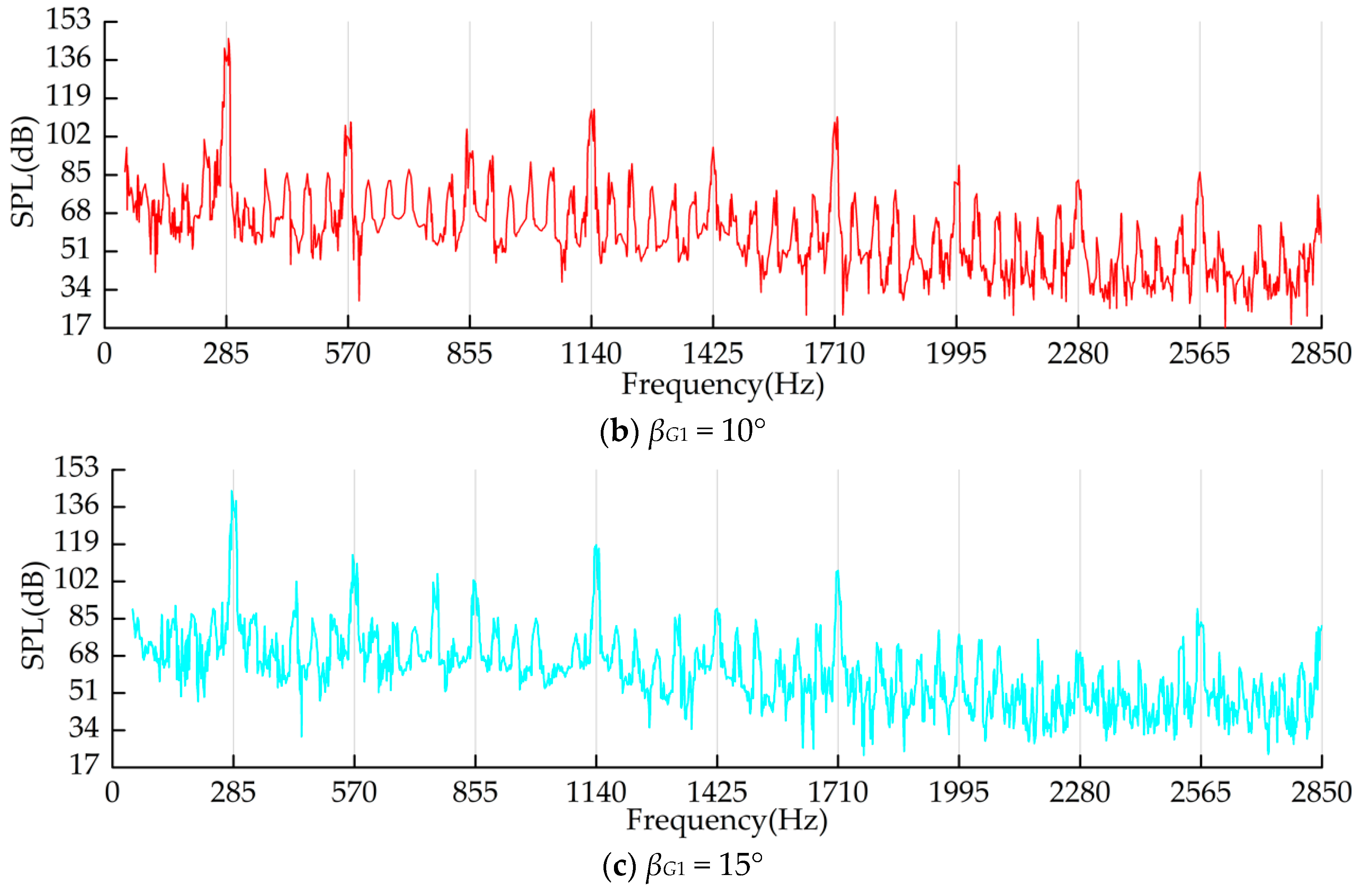
Figure 20.
Frequency response curves of the SPL inside the impeller with different inlet angles of the positive guide vane.
Figure 20.
Frequency response curves of the SPL inside the impeller with different inlet angles of the positive guide vane.
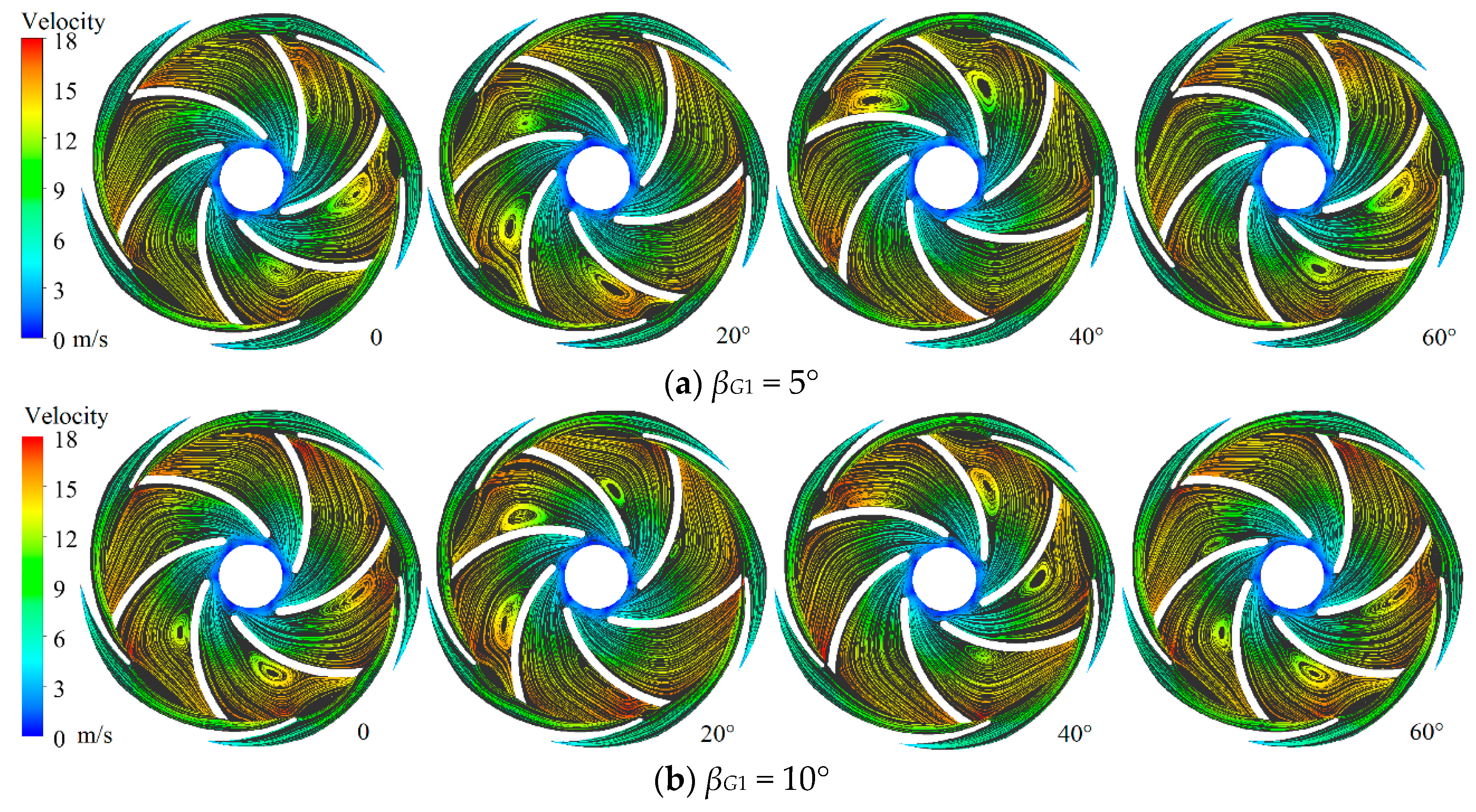
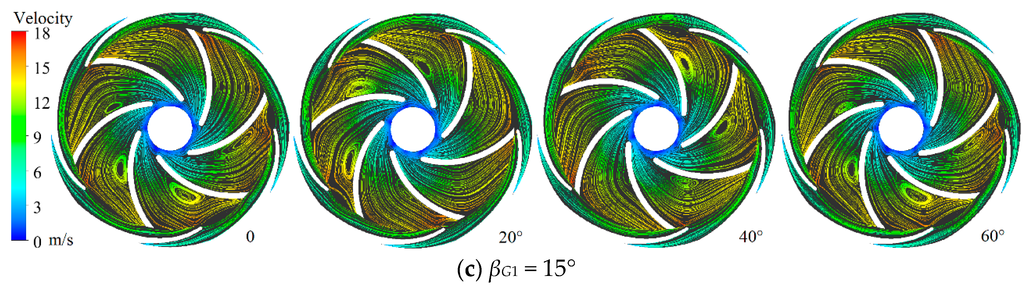
Figure 21.
Evolution processes of the transient flow field inside the impeller and guide vane with different inlet angles of the positive guide vane.
Figure 21.
Evolution processes of the transient flow field inside the impeller and guide vane with different inlet angles of the positive guide vane.
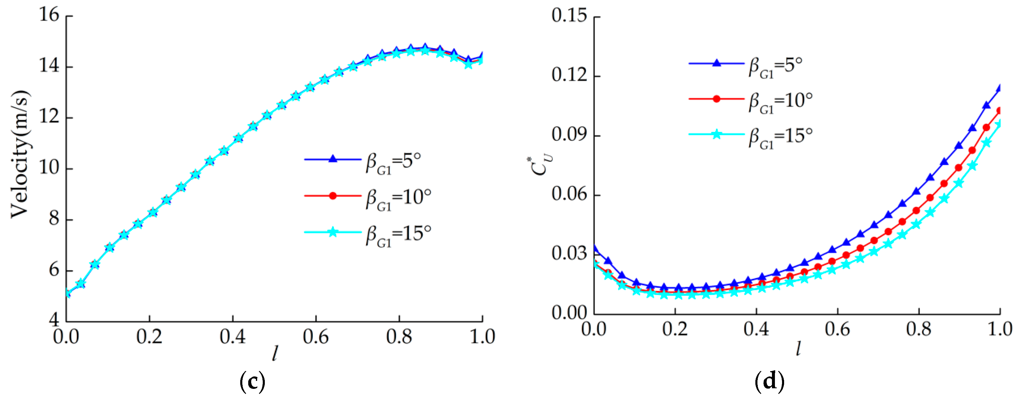
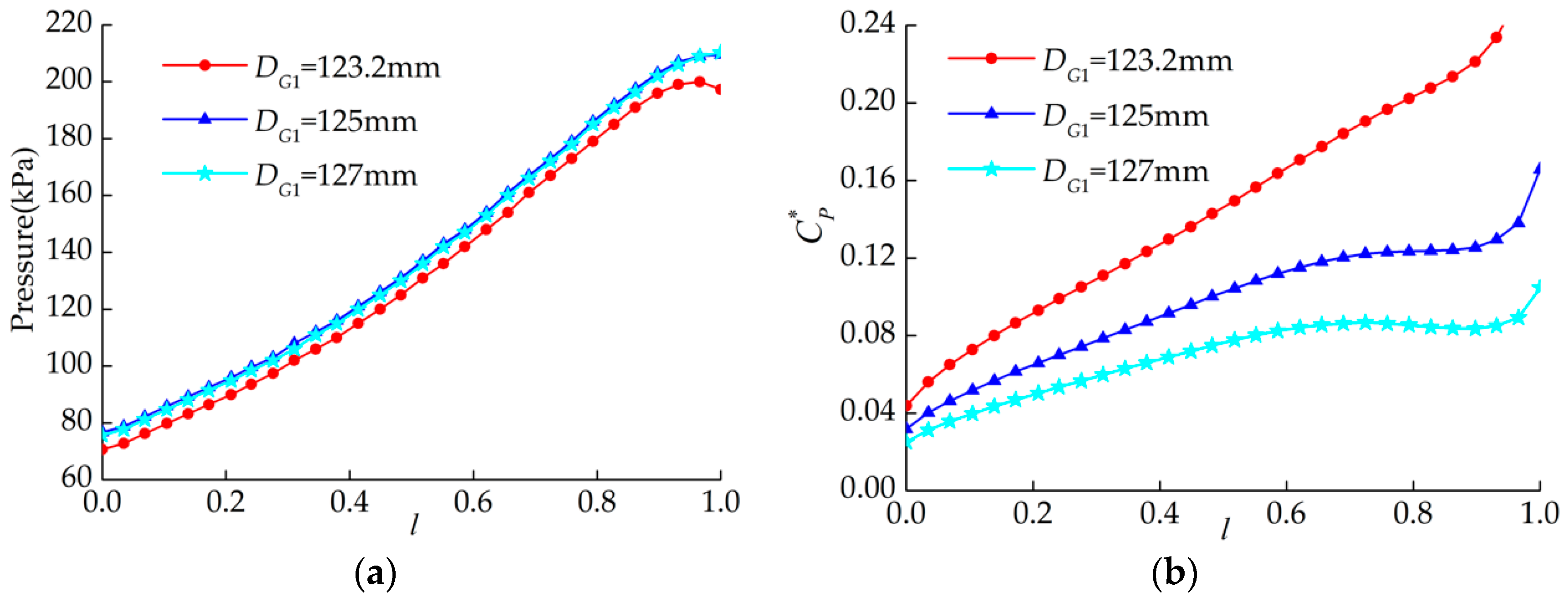
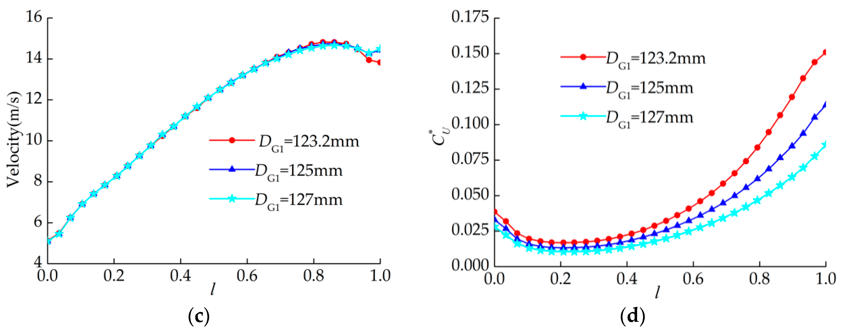
Figure 22.
The time-average and the fluctuation intensity curves of pressure and velocity on the blade surface of the impeller with different inlet diameters of the positive guide vane. (a) The curves of the pressure time-average; (b) the curves of pressure fluctuation intensity; (c) the curves of the velocity time-average; (d) the curves of velocity fluctuation intensity.
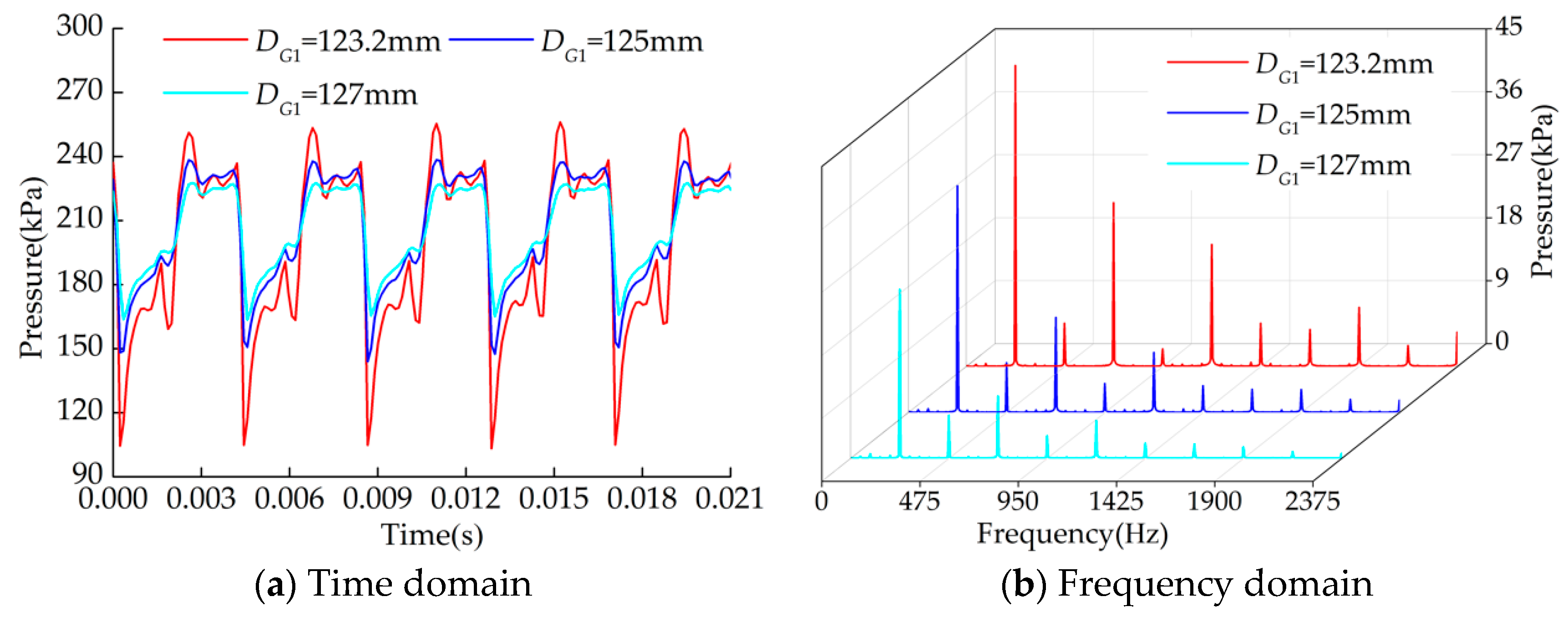
Figure 23.
Frequency response curves of pressure inside the impeller with different inlet diameters of the positive guide vane.
Figure 23.
Frequency response curves of pressure inside the impeller with different inlet diameters of the positive guide vane.
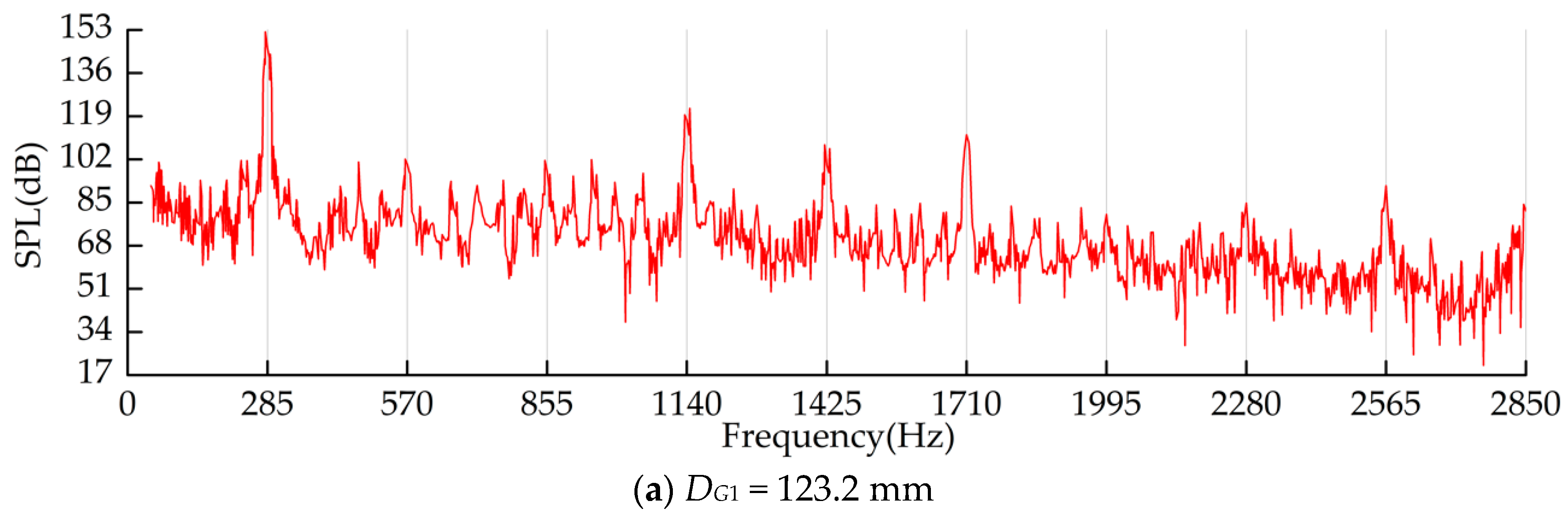
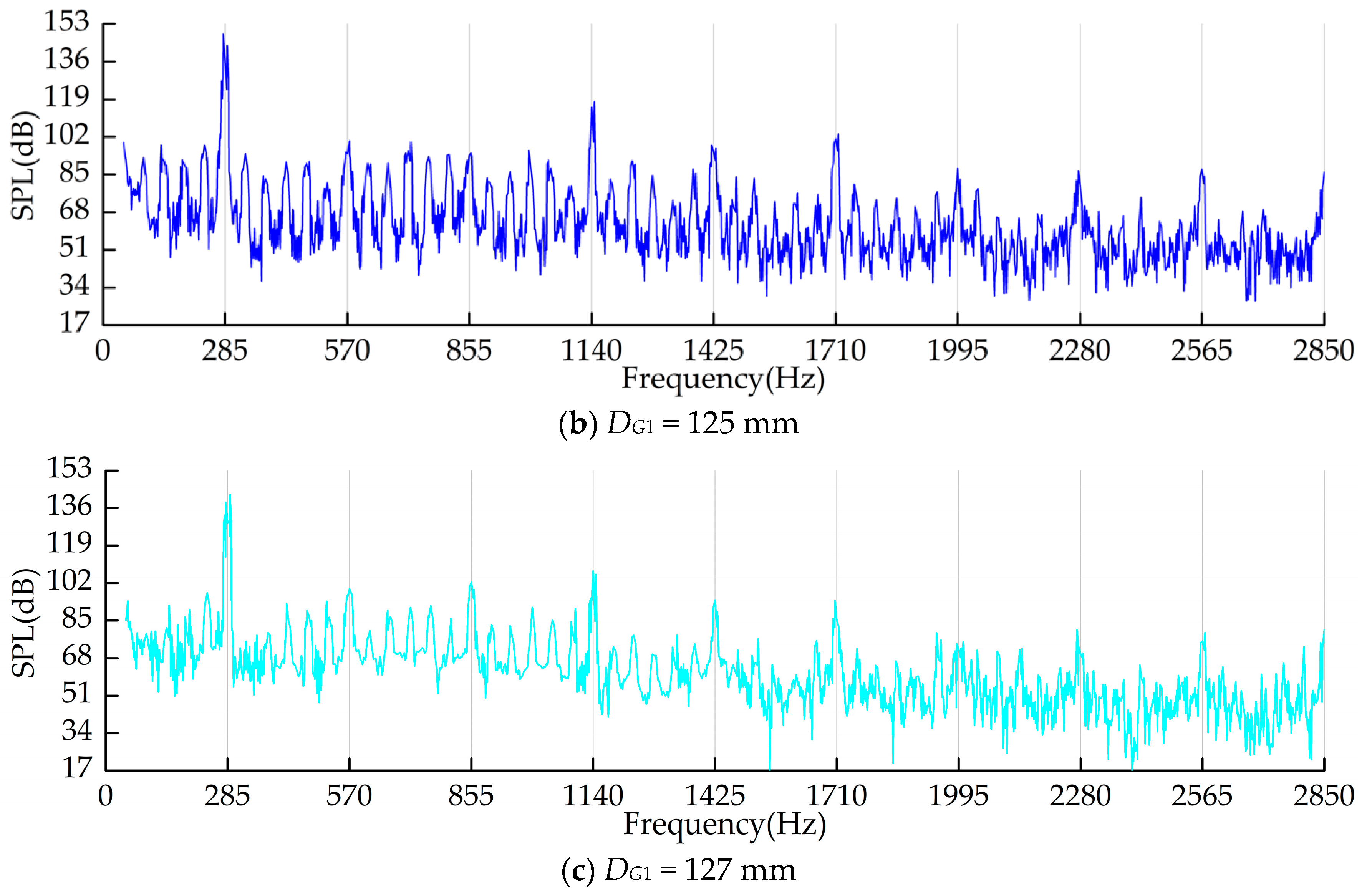
Figure 24.
Frequency response curves of the hydroacoustic SPL inside the impeller with different inlet diameters of the positive guide vane.
Figure 24.
Frequency response curves of the hydroacoustic SPL inside the impeller with different inlet diameters of the positive guide vane.
Figure 25.
Evolution processes of the transient flow field inside the impeller and guide vane with different inlet diameters of the positive guide vane.
Figure 25.
Evolution processes of the transient flow field inside the impeller and guide vane with different inlet diameters of the positive guide vane.
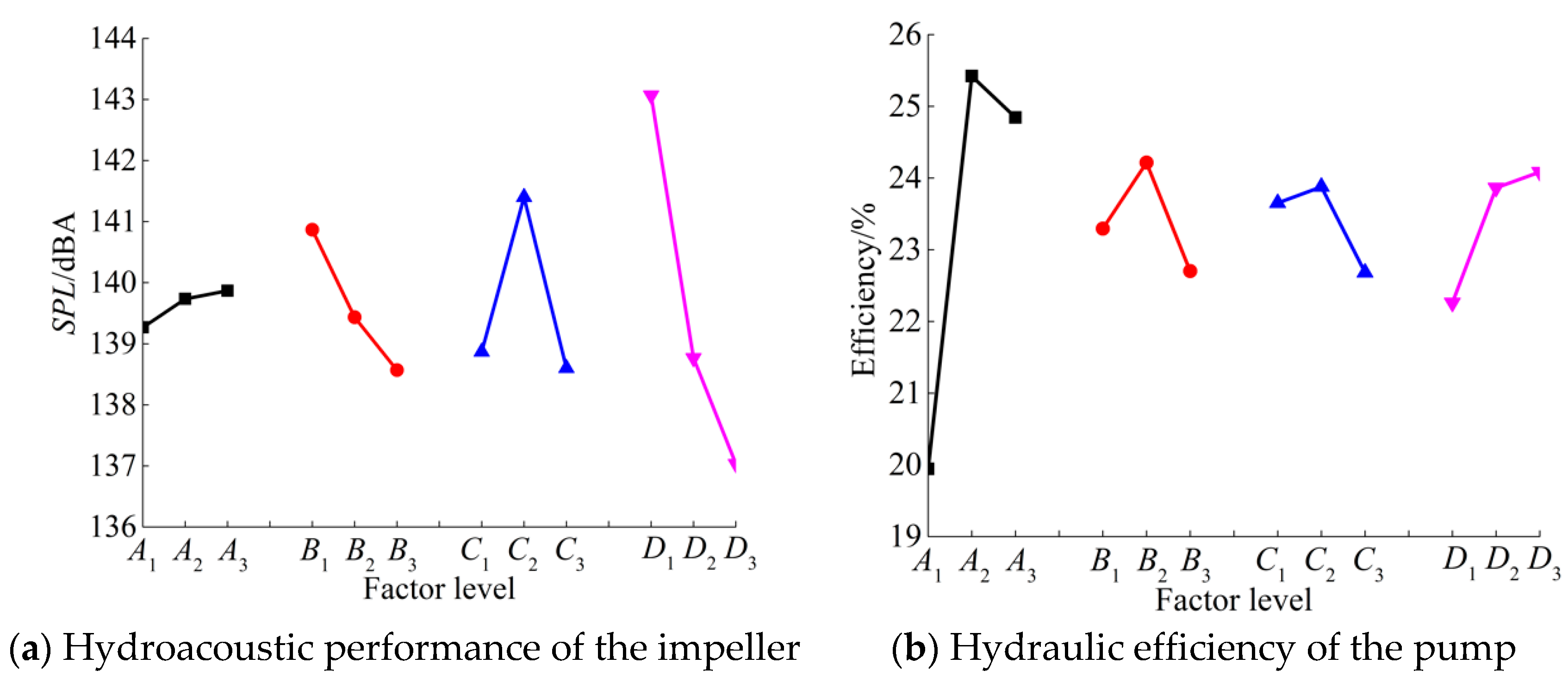
Figure 26.
Effective curves of optimization indexes.
Figure 26.
Effective curves of optimization indexes.
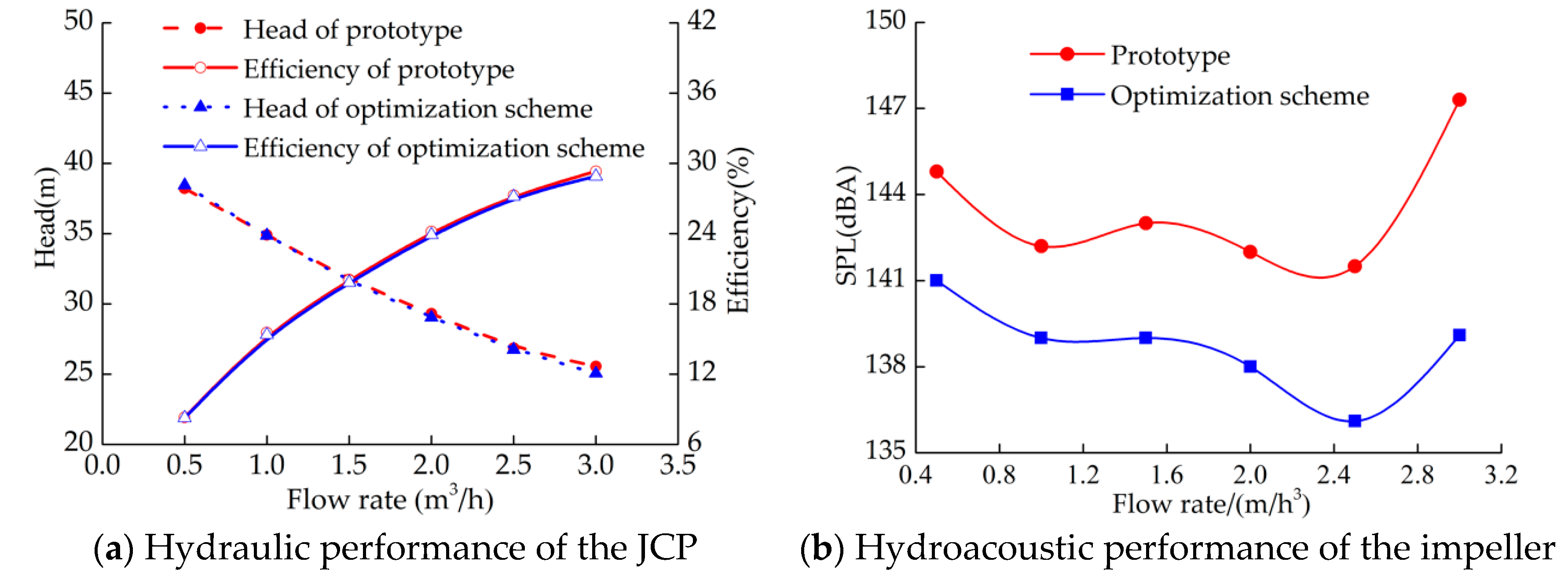
Figure 27.
Performance comparison between the prototype and optimization scheme.
Figure 27.
Performance comparison between the prototype and optimization scheme.
Table 1.
Parameters for the model jet centrifugal pump.
Table 1.
Parameters for the model jet centrifugal pump.
| Components | Parameter | Value |
|---|
| Impeller | Inlet diameter DI1 (mm) | 40 |
| Outlet diameter DI2 (mm) | 123 |
| Blade number Z1 | 6 |
| Blade wrap angle φ1 (°) | 76 |
| Blade outlet width b2 (mm) | 5.3 |
| Guide vane | Inlet diameter DG1 (mm) | 125 |
| Outlet diameter DG2 (mm) | 64 |
| Blade number Z2 | 5 |
Table 2.
The grid independence analyzation.
Table 2.
The grid independence analyzation.
| Schemes | Scheme 1 | Scheme 2 | Scheme 3 | Scheme 4 | Scheme 5 | Scheme 6 |
|---|
| Number of the grid | 1,483,718 | 1,975,598 | 2,526,764 | 3,030,389 | 3,494,674 | 4,046,652 |
| Head (m) | 23.97 | 24.22 | 25.43 | 26.15 | 26.17 | 26.16 |
Table 3.
Data structure of the weight matrix analysis method.
Table 3.
Data structure of the weight matrix analysis method.
| Index Layer | Indices of Experimental Investigation |
|---|
| Factor Layer | K1 | K2 | … | Kn |
| Level Layer | K11K12 … K1m | K21K22 … K2m | … | Kn1Kn2 … Knm |
Table 4.
Main geometric parameters of the original positive guide vane.
Table 4.
Main geometric parameters of the original positive guide vane.
| Parameters | Blade Number Z2 | Wrap Angle φ2 /° | Inlet Angle βG1/° | Inlet Diameter DG1 /mm |
|---|
| Value | 5 | 68 | 5 | 125 |
Table 5.
The influence of guide vanes on the hydraulic and hydroacoustic characteristics of the impeller.
Table 5.
The influence of guide vanes on the hydraulic and hydroacoustic characteristics of the impeller.
Guide Vane
Models | Characteristics of the Impeller | Performance of the Pump |
|---|
| | Energy Head of inlet/m | Energy Head of outlet/m | Energy
increment /m | Shaft Power
/W | Total
SPL/dBA | Water Head/m | Hydraulic Efficiency
/% |
| I | −1.14 | 27.01 | 28.15 | 426.4 | 92.1 | 5.20 | 8.40 |
| II | 4.66 | 30.42 | 25.76 | 631.0 | 128.4 | 21.23 | 23.17 |
| III | 6.51 | 31.09 | 24.58 | 678.1 | 141.6 | 26.85 | 27.27 |
Table 6.
Correlations between the number of guide vanes and hydraulic and hydroacoustic characteristics of the impeller.
Table 6.
Correlations between the number of guide vanes and hydraulic and hydroacoustic characteristics of the impeller.
| Guide Vane Parameter | Characteristics of the Impeller | Performance of the Pump |
|---|
| Blade number Z2 | Energy head of inlet/m | Energy head of outlet/m | Energy increment/m | Shaft power/W | Total SPL/dBA | Water head/m | Hydraulic efficiency/% |
| 3 | 4.10 | 28.86 | 24.76 | 622.4 | 136.4 | 19.76 | 21.87 |
| 5 | 6.51 | 31.09 | 24.58 | 678.1 | 141.6 | 26.85 | 27.27 |
| 7 | 6.18 | 31.27 | 25.09 | 685.2 | 140.7 | 25.78 | 25.91 |
Table 7.
Correlations between the wrap angle of the positive guide vane and the hydraulic and hydroacoustic characteristics of the impeller.
Table 7.
Correlations between the wrap angle of the positive guide vane and the hydraulic and hydroacoustic characteristics of the impeller.
| Guide Vane Parameter | Characteristics of the Impeller | Performance of the Pump |
|---|
| Wrap angle φ2 (°) | Energy head of inlet/m | Energy head of outlet/m | Energy increment /m | Shaft power/W | Total SPL/dBA | Water head/m | Hydraulic efficiency/% |
| 52 | 6.02 | 30.03 | 24.01 | 670.2 | 146.9 | 25.43 | 26.13 |
| 68 | 6.51 | 31.09 | 24.58 | 678.1 | 141.6 | 26.85 | 27.27 |
| 84 | 6.32 | 31.52 | 25.20 | 698.4 | 139.8 | 26.25 | 25.89 |
Table 8.
Correlations between the inlet angle of the positive guide vane and the hydraulic and hydroacoustic characteristics of the impeller.
Table 8.
Correlations between the inlet angle of the positive guide vane and the hydraulic and hydroacoustic characteristics of the impeller.
| Guide Vane Parameter | Characteristics of the Impeller | Performance of the Pump |
|---|
| Inlet angle βG1/° | Energy head of inlet/m | Energy head of outlet/m | Energy increment /m | Shaft power/W | Total SPL/dBA | Water head/m | Hydraulic efficiency/% |
| 5 | 6.51 | 31.09 | 24.58 | 678.1 | 141.6 | 26.85 | 27.27 |
| 10 | 6.14 | 30.89 | 24.75 | 676.2 | 138.7 | 25.73 | 26.21 |
| 15 | 5.87 | 30.85 | 24.98 | 676.1 | 136.5 | 24.86 | 25.33 |
Table 9.
Correlations between the inlet diameter of the positive guide vane and the hydraulic and hydroacoustic characteristics of the impeller.
Table 9.
Correlations between the inlet diameter of the positive guide vane and the hydraulic and hydroacoustic characteristics of the impeller.
| Guide Vane Parameter | Hydraulic and Hydroacoustic Characteristics of the Impeller | Hydraulic Performance of the Pump |
|---|
| Inlet diameter DG1 (mm) | Energy head of inlet/m | Energy head of outlet/m | Energy increment /m | Shaft power/W | Total SPL/dBA | Water head/m | Hydraulic efficiency/% |
| 123.2 | 5.89 | 28.85 | 22.96 | 668.5 | 145.3 | 25.06 | 25.82 |
| 125 | 6.51 | 31.09 | 24.58 | 678.1 | 141.6 | 26.85 | 27.27 |
| 127 | 6.39 | 31.56 | 25.17 | 678.2 | 136.2 | 26.75 | 27.17 |
Table 10.
Levels of the orthogonal experimental factors.
Table 10.
Levels of the orthogonal experimental factors.
| Level | Factors |
|---|
| A/Z2 | B/φ2 | C/βG1 | D/DG1 |
|---|
| 1 | 3 | 52° | 5° | 123.2 mm |
| 2 | 5 | 68° | 10° | 125 mm |
| 3 | 7 | 84° | 15° | 127 mm |
Table 11.
Orthogonal experimental schemes and results.
Table 11.
Orthogonal experimental schemes and results.
| Number | A/Z2 | B/φ2 | C/βG1 | D/DG1 | Total SPL of Impeller/LP (dBA) | Water Head/H (m) | Hydraulic Efficiency/η (%) |
|---|
| 1 | 1 | 1 | 1 | 1 | 143.2 | 15.99 | 18.94 |
| 2 | 1 | 2 | 2 | 2 | 140.0 | 20.10 | 21.69 |
| 3 | 1 | 3 | 3 | 3 | 134.6 | 16.33 | 19.20 |
| 4 | 2 | 2 | 1 | 3 | 136.2 | 26.42 | 27.16 |
| 5 | 2 | 3 | 2 | 1 | 143.9 | 23.66 | 24.05 |
| 6 | 2 | 1 | 3 | 2 | 139.1 | 24.28 | 25.06 |
| 7 | 3 | 3 | 1 | 2 | 137.2 | 23.88 | 24.85 |
| 8 | 3 | 1 | 2 | 3 | 140.2 | 25.72 | 25.89 |
| 9 | 3 | 2 | 3 | 1 | 142.1 | 23.25 | 23.79 |
Table 12.
Results of range analysis.
Table 12.
Results of range analysis.
| | Total SPL of the Impeller/LP (dBA) | Hydraulic Efficiency of the Pump/η (%) |
|---|
| Factor | k1 | k2 | k3 | s | k1 | k2 | k3 | s |
| A | 139.3 | 139.7 | 139.9 | 0.60 | 19.94 | 25.42 | 24.84 | 5.48 |
| B | 140.9 | 139.4 | 138.6 | 2.30 | 23.29 | 24.21 | 22.70 | 1.20 |
| C | 138.9 | 141.4 | 138.6 | 2.80 | 23.65 | 23.88 | 22.68 | 1.51 |
| D | 143.1 | 138.8 | 137.0 | 6.03 | 22.26 | 23.86 | 24.08 | 1.82 |


