Diatom Species Richness in Swiss Springs Increases with Habitat Complexity and Elevation
by
 ,
,
Lukas Taxböck
1,2,*, 
Dirk Nikolaus Karger
3,
Michael Kessler
2,
Daniel Spitale
4 and
Marco Cantonati
4
1
Aachwiesen 8, 8599 Salmsach, Switzerland
2
Departement of Systematic and Evolutionary Botany, University of Zurich, Zollikerstrasse 107, 8008 Zurich, Switzerland
3
Swiss Federal Research Institute WSL, Zürcherstrasse 111, 8903 Birmensdorf, Switzerland
4
MUSE-Museo delle Scienze, Limnology & Phycology Section, Corso del Lavoro e della Scienza 3, 38123 Trento, Italy
*
Author to whom correspondence should be addressed.
Water 2020, 12(2), 449; https://doi.org/10.3390/w12020449
Submission received: 31 December 2019
/
Revised: 26 January 2020
/
Accepted: 3 February 2020
/
Published: 7 February 2020
(This article belongs to the Special Issue Multiplicity, Characteristics, Main Impacts, and Stewardship of Natural and Artificial Freshwater Environments: Consequences for Biodiversity Conservation)
Abstract
:Understanding the drivers of species richness gradients is a central challenge of ecological and biodiversity research in freshwater science. Species richness along elevational gradients reveals a great variety of patterns. Here, we investigate elevational changes in species richness and turnover between microhabitats in near-natural spring habitats across Switzerland. Species richness was determined for 175 subsamples from 71 near-natural springs, and Poisson regression was applied between species richness and environmental predictors. Compositional turnover was calculated between the different microhabitats within single springs using the Jaccard index based on observed species and the Chao index based on estimated species numbers. In total, 539 diatom species were identified. Species richness increased monotonically with elevation. Habitat diversity and elevation explaining some of the species richness per site. The Jaccard index for the measured compositional turnover showed a mean similarity of 70% between microhabitats within springs, whereas the Chao index which accounts for sampling artefacts estimated a turnover of only 37%. Thus, the commonly applied method of counting 500 valves led to an undersampling of the rare species and might need to be reconsidered when assessing diatom biodiversity.
1. Introduction
Understanding the factors that drive gradients of species richness is one of the major challenges of ecological and biogeographical research. To investigate patterns of species richness and the related environmental drivers, elevational gradients have received considerable attention in the last decade, and have become firmly established as a replicable methodology [1,2,3,4]. Elevational richness patterns across a wide range of taxa can show a variety of response shapes to the gradient, from monotonic declines to more or less hump-shaped patterns, with maximum richness at some intermediate point of the gradient [3,4,5]. For microorganisms, patterns of species richness along elevational gradients can, however, contrast with those of macroorganisms [6] and the determinants of elevational distributions of microorganism species richness are still poorly understood. Studying microorganisms along elevational gradients might therefore provide important insights into the processes determining species richness along elevational gradients. Moreover, different aspects of biodiversity can be driven by different main factors: Wang et al. [7] for instance, found for stream diatom assemblages along elevational gradients in Asia and Europe that richness was mostly related to pH, while evenness was mostly explained by total phosphorus.
Diatoms are an important group of microorganisms, being one of the most diverse groups of single-celled algae that are distributed worldwide in nearly all aquatic ecosystems. They show a high variation in ecological requirements and are characterized by an outer silica frustule that stays preserved over long periods of times [8]. These characteristics make them valuable environmental indicators in studies of climate change, acidic precipitation, and water quality [9]. Additionally, diatoms are important primary producers in aquatic ecosystems, with an estimated share of up to 20% of the worldwide primary production [10]. Despite their valuable contributions to ecosystem functioning and their value as ecological indicators, the distribution and drivers of diatom diversity remain poorly understood. Diatoms were considered to be cosmopolitan, with only little dispersal limitation [11,12]. Their high dispersal abilities lead to a strong connection between the environment and species composition and diversity, since species can easily reach favorable habitats. The statement of cosmopolitism, however, has become controversial, due to increasing evidence of endemic species [13,14,15,16,17] as well as the problem to identify environmental drivers for diversity and distribution. Moreover, using combined datasets covering very large spatial scales, several studies have shown that population divergence in diatoms apparently takes place over distances of 100 s to 1000 s of kilometers, and that dispersal-related factors generally fail to explain part of the variation in the diatom community structure, with the exception of datasets that span more than 2000 km [18,19]. Studying different ecoregions in Finland in a study area with a diameter of about 300 km, Teittinen and Soininen [20] showed for diatom assemblages in springs that spatial factors were of minor importance as compared to environmental filtering. By studying elevational patterns of different microbial groups (including diatoms) in subarctic ponds, Teittinen et al. [21] confirmed that aquatic autotrophs are primarily controlled by environmental filtering.
In springs, where diatoms are often the most important primary producers, diatom diversity can be influenced by a variety of environmental factors. Water current velocity and the availability of semiaquatic habitats are probably the most important environmental variables driving species richness for flowing and seepage springs [22,23,24]. Additionally, many studies, including Cantonati et al. [25] for flowing springs of the south-eastern Alps, and [26] for spring fens of the western Carpathians, showed that pH, conductivity, elevation, nitrate, sulphate, and total phosphorus are important environmental determinants of diatom richness. Additionally, calcium ion concentration and nitrate concentrations can affect diatom species richness as shown for anthropogenically altered springs in Poland [27]. A common point of all studies investigating environmental drivers of diatom diversity is that all these studies revealed that environmental variables can only partly explain diatom diversity.
Yet, biodiversity is not only about species numbers but also about spatial changes in species composition. Compositional turnover can be influenced by a variety of factors including stochastic (random) and deterministic processes of community assembly [28,29,30,31,32] as well as species pool sizes [17], and hence, by factors that vary at large extents and trickle down to the local scale [33]. Such factors include habitat area [34], the evolutionary history of lineages and regions [35,36,37,38], the cumulative effects of stochastic variation [39], or sampling constrains [40,41,42,43,44]. The most important factors influencing compositional turnover of diatom communities are presumably geogenic variables: pH, conductivity, alkalinity [7,21,45]; hydrological stability [22,24,45]; substrate-particle size, light availability, temperature, nitrate, and phosphorus [7,22,25]; or substrate types [25,46].
Finally, the perception of all these patterns is also influenced by sampling strategy. In particular, since typically in any biotic community a few species are common while most species are rare, incomplete sampling will lead to underestimation of total species numbers and as well to biases in the calculation of community similarity between sites [47]. These biases can be countered by a number of statistical approaches, e.g., [48], but their influence on our understanding of patterns of diatom diversity remain poorly explored.
Here, we investigated changes in species richness and turnover in spring diatom communities in near-natural springs along an elevational gradient in the Swiss Alps. The aims of the study were to answer the following questions: What is the elevational pattern of diatom richness in springs in the Alps? Which environmental variable is the most influential on species turnover between the habitats? Does restricted sampling lead to higher similarities between habitats due to the undersampling of the communities natural to each habitat, or does it lead to lower similarity between habitats, as despite communities being sufficiently sampled, rare species are missing from the sample? We therefore aimed to investigate the influence of sampling constrains on environmental determinism on turnover rates along an altitudinal gradient to move a step forward in disentangling the drivers of diatom community composition.
2. Materials and Methods
2.1. Study Area and Sites
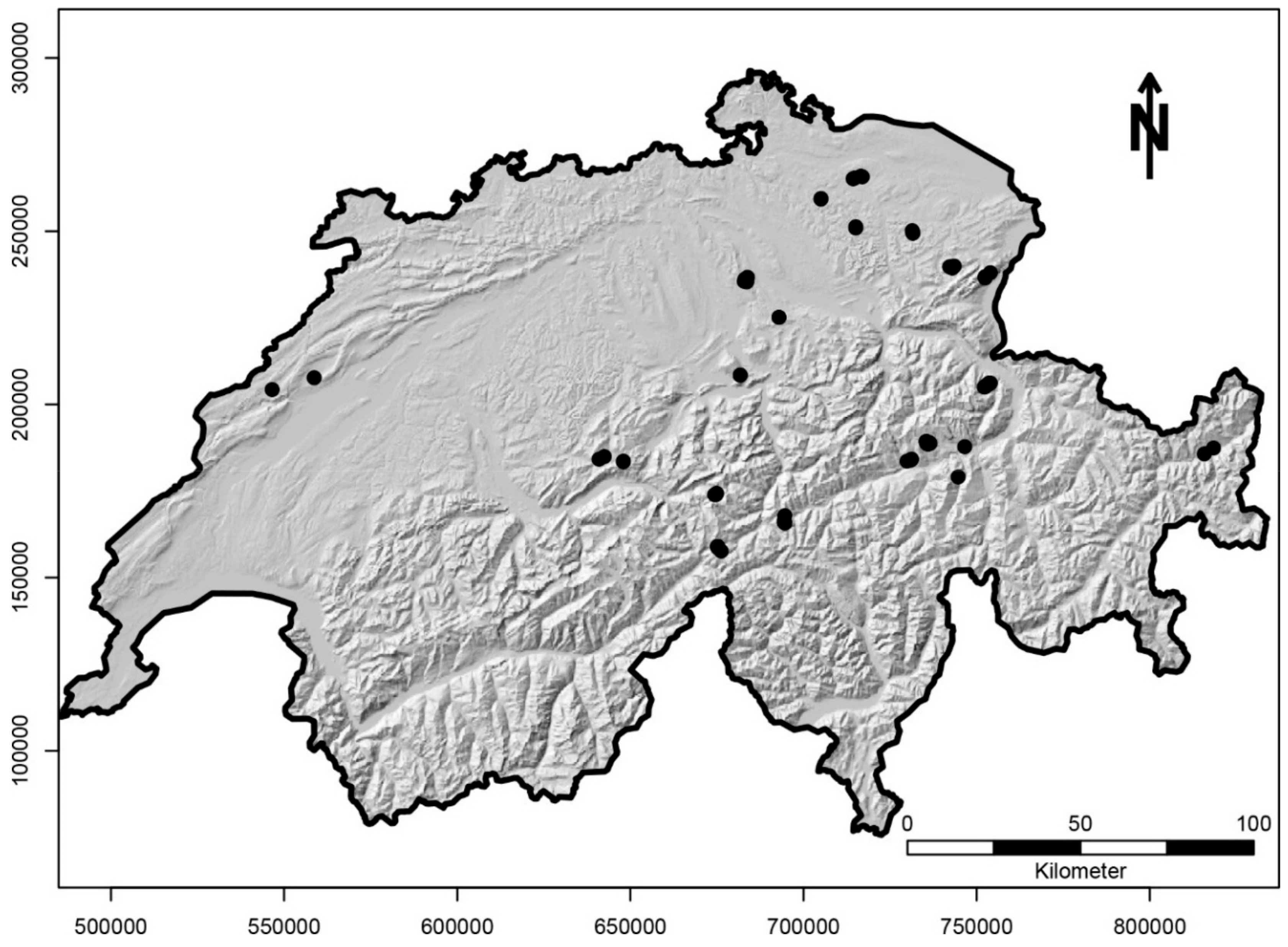
Sampling was undertaken in 71 near-natural springs across Switzerland at elevations from 520 m to 2527 m a.s.l. (Figure 1) and covering different spring types. We distinguished between rheocrenes (n = 29; flowing springs), rheohelocrenes (n = 10; seepage springs on steep slopes), helocrenes (n = 15; seepage springs), limnocrenes (n = 1; pool springs), linear springs (n = 3; seepage springs with a fluctuating outflow, e.g., depending on precipitation), hygropetric springs (n = 2; seepage springs flowing over rocks), and walled springs (n = 6; altered springs with a rheocrenic character, e.g., water catchment, outflow through pipes, but the springs remains mostly in a near-natural character). Near-natural springs are optimal study systems for many groups of organisms [49,50,51,52] including diatoms [53] since they cover a variety of microhabitats on a small spatial scale, show only limited anthropogenic disturbance, and often reveal high species richness, e.g., [25,50]. Permanent springs are known to be stable habitats, since a number of environmental factors are determined by the aquifer feeding the spring [54]. However, springs can vary greatly among each other, even at a local scale, in habitat diversity and physical and chemical parameters, e.g., [50].
2.2. Field Sampling
We defined five different microhabitats that were sampled if present in each spring: stones, sediment, bryophytes, leaf litter, and filamentous green algae (Table S2). We collected 175 samples in 71 springs. From every habitat, we sampled periphyton to determine species richness and community composition in a minimum of three different spots within a spring. Stones offer a steady habitat to benthic diatoms, can vary in size, and are usually exposed to the running water. Sampling of the stone habitat was conducted by sampling 5–10 stones in each spring (depending on their size), or if only small gravel (ø < 2 cm) was available, 10–15 small stones were taken as a whole. Sediment is irregularly distributed in springs and is often accumulated in areas of still water. Sediment consists mainly of sand and silt but also organic detritus. Sampling of the sediment habitat was conducted by taking circa 10–20 cm3 of sediment from the surface. Bryophytes build canopies along the spring’s edges or around the spring’s mouth over the whole spring diameter. On these bryophytes, epiphytic diatoms are found while among the stems and leaves also planktic diatoms can be trapped. Filamentous green-algae build small patches of densely growing filaments, offering epiphytic diatoms a habitat. Leaf litter are dead leaves fallen from the trees around the spring. Epiphytic or diatoms with low light requirements can be found there. Bryophyte habitat, filamentous green-algae habitat, and leaf litter habitat was sampled by taking between 30–40 cm3 of each habitat as a whole.
Sampling was conducted during the summer months 2009–2011, and every spring was only sampled once. In walled springs, rheocrenes, and rheohelocrenes, spring area was delimited where bryophyte canopies stopped growing. Helocrenes and hygropetric and linear springs were sampled on a stretch of maximal 3–5 times the spring mouth diameter, and the limnocrene was delimited by the pool’s surface size.
2.3. Laboratory Analyses
Samples were preserved in a 4% formaldehyde solution. Samples from calcareous bedrock, small gravel (ø < 2 cm), bryophytes, filamentous green-algae and leaf litter were treated with hydrochloric acid to remove carbonates and to detach the adhering diatoms. The cleaned substrates and larger remaining particles were filtered out with a small meshed sieve. Diatom frustules were cleaned from organic matter in concentrated sulphuric acid and potassium nitrate, followed by washing with deionized water [55]. Cleaned diatom frustules were mounted on microscope slides with Naphrax (refractive index = 1.74), two permanent slides were mounted per sample. Species were identified using species descriptions and revisions [56,57,58,59,60,61,62,63,64,65,66,67,68,69,70,71].
2.4. Species Richness and Compositional Turnover
We assessed species richness from subsamples (n = 175) by counting 500 valves per slide. We calculated compositional turnover in species communities between microhabitats using two different methods. First, we calculated compositional turnover using the Jaccard index based on the observed species richness from the subsamples of each habitat. The equation for the Jaccard index is computed as 2B = (1 + B) where B is the Bray-Curtis dissimilarity, that is:
Since our richness data is constrained by a maximum of 500 individuals per sample, we also used the Chao based index for compositional turnover [48] to account for incomplete sampling. This allows us to distinguish if dissimilarities between different microhabitats are solely based on sampling constrains. Chao index tries to take into account the number of unseen species pairs. The function vegdist of the package Vegan in R [72], implements a Jaccard type index defined as djk = 1 − UjUk = (Uj + Uk − UjUk), where Uj = Cj/Nj + (Nk − 1)/Nk × a1/(2a2) × Sj/Nj, and similarly for Uk. Here, Cj is the total number of individuals in the species of site j that are shared with site k, Nj is the total number of individuals at site j, a1 (and a2) are the number of species occurring in site j that have only one (or two) individuals in site k, and Sj is the total number of individuals in the species present at site j that occur with only one individual in site k [70].
2.5. Explanatory Factors
We used a set of 10 explanatory factors to describe species richness. Current velocity and shading conditions were estimated according to five-point scales [71]. Conductivity [µS cm−1], pH, dissolved oxygen [%], and temperature [°C] were measured on site using a portable digital probe [Hach-Lange HQ40D including LDO (O2), PHC (pH, °C), CDC (µS/cm)]. Nitrate (NO3-N), Total Phosphorus (TP), and Chloride (Cl-) were measured with Hach-Lange cuvette tests.
2.6. Statistical Analyses
We used Poisson regression to model species richness and predictors and beta regression between compositional turnover and predictors. In the case of high residual deviance after model selection, we used a quasi-Poisson distribution. Diversity as well as turnover can be influenced by several factors. We therefore expected to find combined effects of different independent variables in most cases, thus, we used multiple linear regression with all possible variable combinations to build full linear models. We then applied backward variable reduction to avoid overfitting the multiple regression models. Variables were standardized to zero mean and unit variance to account for different measuring units. To investigate possible drivers of compositional turnover, we used beta regression between the respective turnover index and all 10 environmental variables. To avoid overfitting, we did not perform multiple regressions for compositional turnover, since turnover rates between habitats could only be calculated for a subset of all springs due to habitat occurrence within springs (see n in Figure 2. All analyses were conducted using the package ‘vegan’ [72] and ‘betareg’ [73] in R 3.0.0 [74].
3. Results
3.1. Habitat Diversity and Species Richness
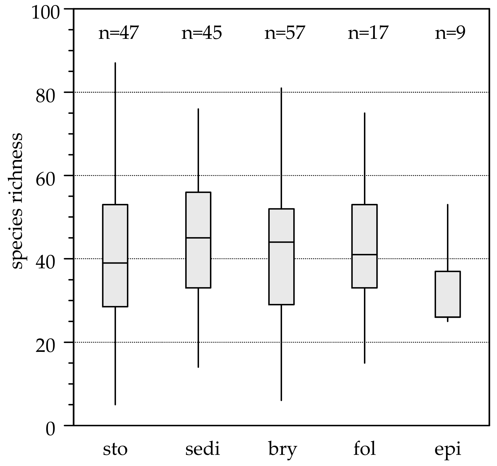
The most abundant microhabitats within springs were stones (n = 47), sediment (n = 45), and bryophytes (n = 57). In lower numbers, we sampled filamentous green-algae (n = 17) and leaf litter (n = 9).
On all substrates, we identified a total of 539 diatom species with an average of 55 species per sampled spring. The lowest species richness (five species) was found in a hygropetric spring with a high mineral content, where only stones were available as substrate. The highest species richness (114 species) occurred in a helocrenic spring with four different substrates (Table S1). Means of species numbers per microhabitat were: stones = 39, sediment = 45, bryophytes = 43, leaf litter = 32, epiphytic on filamentous green-algae = 39 (Figure 3).
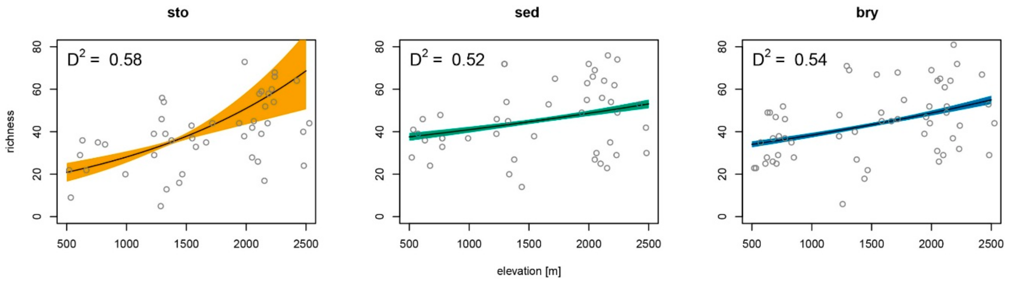
On average, species richness increased monotonically on substrates stones, sediment and bryophytes (Figure 4). The variance, however, was high, resulting in low coefficients of determination.
Habitat diversity (Z = 4.953, p < 0.001) was the strongest explanatory factor of species richness per site; weaker explanatory factors were elevation (Z = 2.221, p < 0.05) and flow velocity (Z = 2.511, p < 0.05) (Table 1). Species richness for single substrates could be explained significantly by elevation for stones (Z = 5.667, p < 0.001), with weaker significance for sediment (Z = 2.188, p < 0.05) and bryophytes (Z = 2.64, p < 0.05). Shading explained species richness significantly for stones (Z = 3.845, p < 0.001) and weaker for leaf litter (Z = −3.59, p < 0.05). Other environmental variables with a weaker statistical significance were conductivity for stones (Z = 3.51, p < 0.01), pH for stones (Z = 3.027, p < 0.01) and filamentous green algae (Z = −2.38, p < 0.05), and total phosphorus for stones (Z = 2.645, p < 0.05) and leaf litter (Z = 6.582, p < 0.01).
3.2. Compositional Turnover
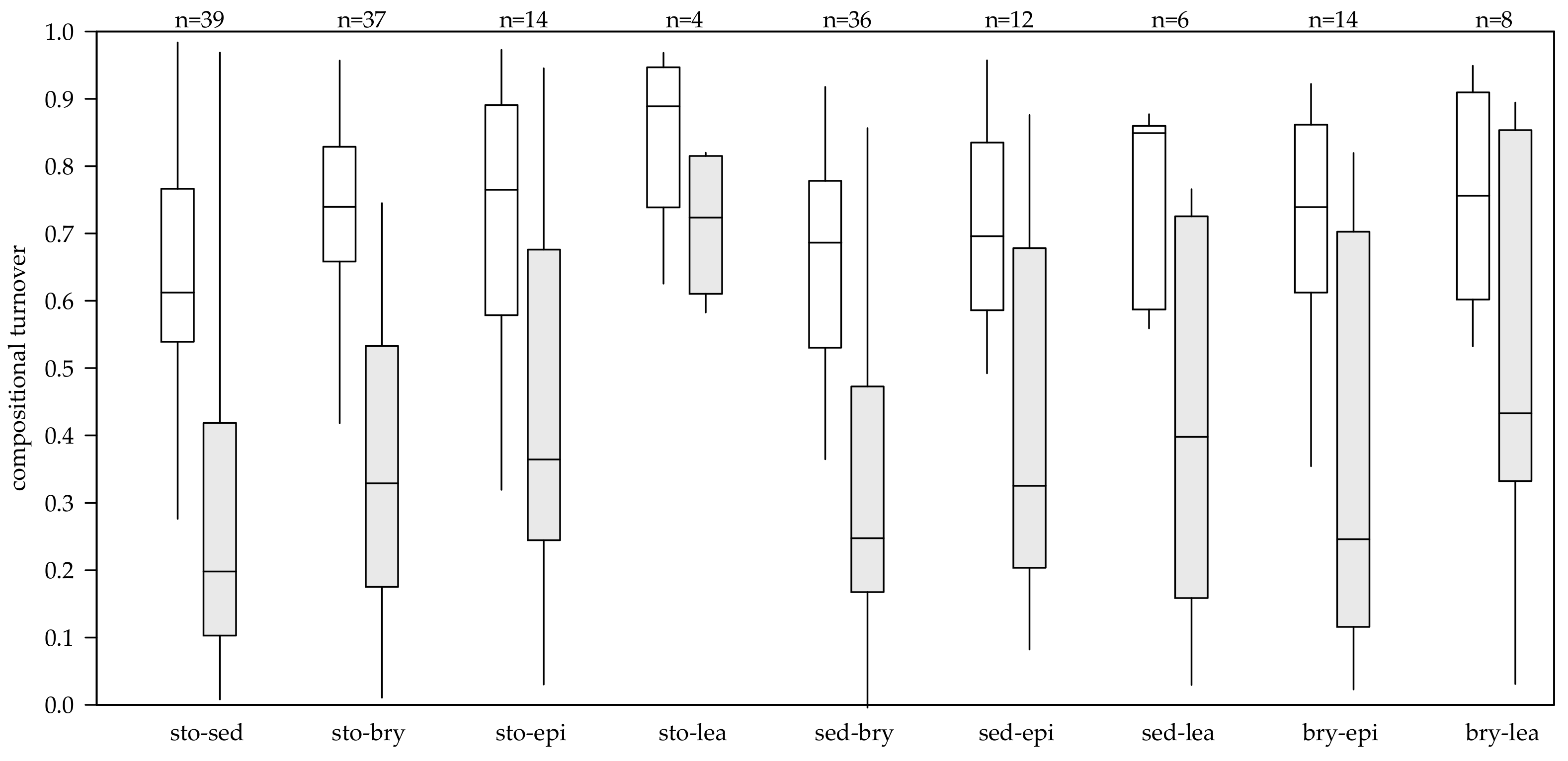
For the possible combinations of substrates, the Jaccard similarity of species richness showed a mean similarity between all microhabitats of 70%. The lowest mean compositional similarity, taking all springs into account, was observed between sediment and bryophytes (=65%), the highest mean compositional similarity was found between stones and leaf litter (=84%) (Table 2).
Measured turnover between microhabitats (sto-sed, sto-bry, sed-bry) showed a monotonic decrease in turnover with elevation, but few of the tested variables explained the compositional turnover between microhabitats. We found no explanation for the compositional turnover between stones and sediment. Between stones and bryophytes, conductivity (Z = 3.101, p = 0.002), total phosphorus (Z = 2.518, p = 0.012), and chloride (Z = −2.368, p = 0.018) were weak explanatory variables. Between sediment and bryophytes, flow velocity (Z = −5.817, p < 0.001) and temperature (Z = −3.694, p < 0.001) explained significantly the measured compositional turnover, while weaker explanation was provided by conductivity (Z = 2.387, p = 0.017), nitrate (Z = −2.156, p = 0.031), and total phosphorus (Z = 2.933, p = 0.003) (Table 3).
The Chao similarity index, which accounts for undersampling, showed a mean similarity of 37% between all microhabitats (Table 2). The minimal mean compositional similarity was found between sediment and bryophytes (33%), the maximum between stones and leaf litter (72%). Estimated turnover between microhabitats (sto-sed, sto-bry, sed-bry) showed a monotonic decrease in turnover with elevation, but few of the tested variables explained the compositional turnover between microhabitats. The best explanation for estimated compositional turnover between stones and sediment were elevation (Z = −2.387, p = 0.001) and flow velocity (Z = −2.798, p = 0.005). Significant explanation between stones and bryophytes was provided by conductivity (Z = 4.200, p < 0.001), pH (Z = −3.383, p < 0.001), total phosphorus (Z = 4.151, p < 0.001), and nitrate (Z = −3.592, p < 0.001). Between sediment and bryophytes, flow velocity (Z = −3.086, p = 0.002) and total phosphorus (Z = 2.171, p = 0.030) were weak explanatory variables for estimated compositional turnover (Table 3).
4. Discussion
Our study revealed relationships between diatom species richness and spring habitat diversity, and environmental variables such as conductivity, flow, light availability and phosphorus, as well as increasing species richness with increasing elevation. At the most general level, our study adds to the evidence that species richness in microorganisms can show contrasting species richness patterns along elevational gradients compared to macro-organisms [7]. Thus, while plants as well as meso- and macrofauna typically show strongly decreasing diversity towards higher elevations in the Alps [75,76] and other mountains [34], we found weakly increasing species richness for diatoms. The lack of a richness decrease, in spite of increasing environmental harshness with elevation, might be due to the “azonal” character of spring habitats that often act in many ways as refugia for different organisms including diatoms [77,78]. Weak elevational richness patterns have also been found in other microorganisms such as bacteria [6]. Other studies on diatom richness have found elevational decreases at low elevation on the Kerguelen Islands [79] and higher elevation in east-central Nepal [80]. By studying elevational patterns of different microbial groups (including diatoms) in subarctic ponds, Teittinen et al. [21] found unimodal elevational patterns for diatoms. Although the elevational pattern of species richness shows an opposing pattern in near natural springs in the Swiss Alps, all diatom studies conducted so far show a high variance in their elevational trends [6,79], pointing towards additional drivers of species richness that might vary independently of elevation, such as habitat diversity and water conductivity.
The number of microhabitats seems to be one of the most important determinants of diatom diversity. Our results in this regard match those of previous studies on diatom substrate specificity from other ecosystems. For example, Smucker et al. [81] in streams in the north-eastern USA missed more potentially occurring species when sampling only stones instead of multiple microhabitats. In boreal rivers in southern Finland, single diatom species showed fidelity to stones, sediments, and plants [82], whereas Cox [46] showed substrate preferences of specific species in German lakes and streams. Species showing substrate preference for stones, wood, sand, and silt were found in rivers across the USA [83]. In Nepalese streams, less than 75% of the total species richness per site was recorded if only one microhabitat was sampled [84]. Cantonati et al. [25] confirmed the relevance of the substrate type as diatom-assemblage determinant in spring habitats. In a global analysis of diatom distribution, Vyvermann et al. [17] showed a connection between local diatom and habitat diversity. The importance of microhabitats for diatom diversity is also underlined by the relatively high rates of turnover between microhabitats within near-natural springs found in our study. Taking into account that undersampling of communities additionally results in underestimating the turnover within diatom communities, the importance of habitat availability as drivers of diatom species richness might still be underestimated.
Focusing on the individual substrates, stones showed the highest statistical support for the relevant environmental determinants. All other substrates only showed limited significance for some of the measured environmental determinants. We hypothesize that stones offer an inert surface and are the most consistent substrate to sample across different spring types, thus resulting in the most standardized data. The other substrates are more variable: sediments are of varying composition of sand, silt, and organic debris, bryophytes are of varying species composition or can accumulate debris, leaf litter is not a permanent substrate, and filamentous green algae are of varying species composition and are not a permanent substrate. Moreover, since sediment usually accumulates in places with still water and since diatom valves and frustules are very resistant to degradation, this substrate integrates parts of different communities that developed over a time span that depends upon the thickness of sediment sampled (taphocoenoses). Accordingly, any underlying relationships with other determinants are probably hidden by the inherent variability of these substrates.
Water conductivity has been detected as environmental determinant of diatom richness and community composition by various other authors in different habitats (e.g., [17,83], in Alpine springs [25], and in carbonate, low-altitude springs [85,86]. Shading or light availability has been mentioned as a relevant environmental driver not only for macroalgae but also for other photosynthetically active organisms [49,50]. Our samples covered a distinct light availability gradient from shaded springs in the forests of the Swiss midlands and the subalpine zone, to the highly light-exposed alpine springs. pH was only recovered as a weak environmental factor for diatom communities on stones. Fránková et al. [26] determined pH as a main environmental variable for diatom species richness, but their studies included very acidic springs in bogs and covered a wider pH gradient.
Although nutrient availability is often mentioned as a driver of diatom diversity [82,83], it played a relevant but secondary role along the studied elevational gradient, as found also in other spring-diatom studies e.g., [25]. Studies revealing nutrients, particularly nitrogen, as important environmental determinants usually cover anthropogenically more intensely impacted areas. Although our datasets comprise springs from some densely populated and intensively used agricultural areas in Switzerland, the water in the aquifers does not transport nutrients, likely because near-natural springs are usually located in areas where groundwater is protected. Lowland springs in Switzerland were all located in forest areas, where the direct impact (e.g., fertilization) by agriculture is small. In contrast, Alpine springs are often affected by cattle-breeding (e.g., cow droppings, trampling damage), but not year-long, and the morphological damages are probably stronger than the impact by nitrate and total phosphorus input.
Our turnover estimates in diatom communities differed by about 30% when we used measured (Jaccard) or estimated (Chao) species turnover. Apparently, the applied method of counting 500 valves led to an undersampling of rare species, leading to an overestimate of community similarity when we only used the measured data (Jaccard similarity). However, it is worth noting that 500 valves counted for each sample is a figure that is equal or higher than that adopted by many diatom studies in Europe (e.g., [87]). Gerecke et al. [88], counting 450 valves per sample, found that diatom species accumulation curves for several springs were still increasing after many years of annual sampling in the frame of long-term ecological research. This suggests that rare species could be of particular interest and that sampling constrains can pose a problem when investigating turnover rates in diatom communities.
When taking environmental factors into account, species turnover between single substrates revealed shading, elevation, and flow rate as important environmental determinants of turnover rates. Yet, only shading was important for the measured species turnover between all microhabitats, although it was less important for the turnover of estimated species composition. For the photoautotrophic diatoms, light availability seems to be an important environmental factor for the dominating species, but for the rare species these factors seem to become more stochastic. Elevation showed some influence on the compositional turnover between stones and sediment, which might be explained with stronger similarities between stones and the sand-dominated sediment than between stones and bryophytes. Turnover rate between stones and sediment and stones and bryophytes was related to water flow rate which seems to select for specific diatom species that do not get washed out of the respective habitat, leading to higher similarity at higher flow rates. Other environmental variables were important only for the compositional turnover of different microhabitat pairs, and were also different for measured Jaccard dissimilarity and estimated Chao dissimilarity. An interpretation might be that the commonly known environmental variables, such as conductivity, pH, flow velocity, and temperature, may select the dominating diatom species on the different substrates, but these variables may not be so important for rare species.
Overall, our results unveiled relationships that are in good agreement with previously shown features: highest species richness in springs on siliceous as compared to carbonate substrate, with siliceous sites located on average at higher elevations than carbonate sites [25]; highest number of diatom taxa in helocrenic springs on siliceous substrate (e.g., [88]); bryophytes have more species as substrate than stones; elevation among the most relevant structuring variables for diatom communities on both stones and bryophytes [25]; geogenic variables (pH, conductivity) as the strongest environmental determinants [21,25]. However, unlike Cantonati and Spitale [22], who could only explain about 3% of the variance with microhabitats, most of our variance was explained by microhabitats. This might be explained by our study which contained five different microhabitats, not only stones and bryophytes.
In relation to conservation purposes and the currently-applied rapid assessment methodologies of diatom richness, problems might arise when using restricted sampling in studies of community composition of diatoms. It is known that rare species are overlooked in limited counting of samples [89], and studies investigating diatom biodiversity without sampling constraint have revealed impressively high species numbers [15] compared to standardized water quality assessment methods. The counting methods applied in water-quality assessment record well known and common species, whereas rare and less distributed species have been neglected thus far. However, there is a potential for the use of rare species for better understanding of ecosystem health [90]. Knowing that species turnover between substrates is underestimated due to sampling constraints, to guarantee more complete floras from oligotrophic environments, diatom biodiversity sampling should additionally focus on rare taxa. It remains unclear why these rare taxa occur at a certain location. Cross contamination was tried to be avoided by cleaning sampling gear between the substrates and the sites. Perhaps these rare taxa are there by chance and disappear within short time slots. Considering how species accumulation curves become flatter with increasing sampling, it is perhaps necessary to count several thousand valves to get a standardized definition of the term “rare taxa”. This is probably not feasible because it is too time consuming. The qualitative method of looking additionally a given time, e.g., 10 min, to account as many rare taxa as possible seems to be more feasible.
In conclusion, we found that species richness of diatoms in springs increases with increasing elevation and that habitat diversity and conductivity are important factors for diatom diversity along elevational gradients. The undersampling rather leads to an underestimation in turnover rates by missing rare species from the sample. Turnover also showed an elevational trend, corresponding with the increasing species richness with elevation.
Supplementary Materials
The following are available online at https://www.mdpi.com/2073-4441/12/2/449/s1, Table S1: Range of environmental factors of the sampled springs; Table S2: Description of the sampled microhabitats.
Author Contributions
Conceptualization, T.L., M.C., K.D.N., and K.M.; methodology, T.L., K.D.N., K.M., and M.C.; software, K.D.N.; formal analysis, S.D., T.L., and K.D.N.; investigation, T.L.; resources, T.L.; data curation, T.L.; writing—original draft preparation, T.L.; writing—review and editing, T.L., M.C., K.D.N., K.M., and S.D.; visualization, T.L.; supervision, M.C. All authors have read and agreed to the published version of the manuscript.
Funding
T.L. was funded by Klaus-Hermann Stiftung, Claraz-Schenkung and the University of Zurich. M.C. was partially funded by the Autonomous Province of Trento while contributing to this study. K.D.N. was partly funded by the Swiss National Foundation (SNF) Grant Number 148691.
Acknowledgments
We thank Rafael Wüest for the R code to generate the Swiss map. Additionally, we thank the anonymous reviewers for their helpful suggestions to improve the first version of the paper.
Conflicts of Interest
The authors declare no conflict of interest.
References
- Kluge, J.; Kessler, M.; Dunn, R.R. What drives elevational patterns of diversity? A test of geometric constraints, climate and species pool effects for pteridophytes on an elevational gradient in Costa Rica. Glob. Ecol. Biogeogr. 2006, 15, 358–371. [Google Scholar] [CrossRef]
- Lomolino, M.V. Elevation gradients of species-density: Historical and prospective views. Glob. Ecol. Biogeogr. 2001, 10, 3–13. [Google Scholar] [CrossRef]
- Rahbek, C. The elevational gradient of species richness: A uniform pattern? Ecography 1995, 18, 200–205. [Google Scholar] [CrossRef]
- Rahbek, C. The role of spatial scale and the perception of large-scale species-richness patterns. Ecol. Lett. 2005, 8, 224–239. [Google Scholar] [CrossRef]
- Grytnes, J.-A.; McCain, C.M. Elevational Trends in Biodiversity. In Encyclopedia of Biodiversity; Elsevier: Amsterdam, The Netherlands, 2007; pp. 1–8. [Google Scholar]
- Wang, J.; Soininen, J.; Zhang, Y.; Wang, B.; Yang, X.; Shen, J. Contrasting patterns in elevational diversity between microorganisms and macroorganisms. J. Biogeogr. 2011, 38, 595–603. [Google Scholar] [CrossRef]
- Wang, J.; Meier, S.; Soininen, J.; Casamayor, E.O.; Pan, F.; Tang, X.; Yang, X.; Zhang, Y.; Wu, Q.; Zhou, J.; et al. Regional and global elevational patterns of microbial species richness and evenness. Ecography 2017, 40, 393–402. [Google Scholar] [CrossRef]
- Round, F.E.; Crawford, R.M.; Mann, D.G. The diatoms. In Biology & Morphology of the Genera; Cambridge University Press: Cambridge, UK, 1990; p. 747. [Google Scholar]
- Smol, J.P.; Stoermer, E.F. The Diatoms: Applications for the Environmental and Earth Sciences, 2nd ed.; Cambridge University Press: Cambridge, UK, 2010; p. 686. [Google Scholar]
- Mann, D.G.; Droop, S.J.M. Biodiversity, biogeography and conservation of diatoms. Hydrobiologia 1996, 336, 19–32. [Google Scholar] [CrossRef]
- Baas Becking, L.G.M. Geobiologie of Inleiding tot de Milieukunde; W. P. Van Stockum & Zoon: The Hague, The Netherlands, 1934. [Google Scholar]
- Finlay, B.J.; Clarke, K.J. Ubiquitous dispersal of microbial species. Nature 1999, 400, 828. [Google Scholar] [CrossRef]
- Bouchard, G.; Gajewski, K.; Hamilton, P.B. Freshwater diatom biogeography in the Canadian Arctic Archipelago. J. Biogeogr. 2004, 31, 1955–1973. [Google Scholar] [CrossRef]
- Hustedt, F. Süßwasser-Diatomeen des indomalayischen Archipels und der Hawaii-Inseln. Nach dem Material der Wallacea-Expedition. Int. Rev. Hydrobiol. 1942, 42, 1–252. [Google Scholar] [CrossRef]
- Lange-Bertalot, H.; Metzeltin, D. Indicators of oligotropy. In 800 Taxa Representative of Three Ecologically Distinct Lake Types Carbonate Buffered, Oligodystrophic, Weakly Buffered Soft Water; Koeltz: Königstein, Germany, 1996; p. 390. [Google Scholar]
- Lowe, R.L.; Kociolek, J.P. New and rare diatoms from “Great-Smoky-Mountains-National-Park”. Nova Hedwig. 1984, 39, 465–476. [Google Scholar]
- Vyverman, W.; Verleyen, E.; Sabbe, K.; Vanhoutte, K.; Sterken, M.; Hodgson, D.A.; Mann, D.G.; Juggins, S.; Van De Vijver, B.; Jones, V.; et al. Historical processes constrain patterns in global diatom diversity. Ecology 2007, 88, 1924–1931. [Google Scholar] [CrossRef] [PubMed]
- Vanormelingen, P.; Verleyen, E.; Vyverman, W. The diversity and distribution of diatoms: From cosmopolitanism to narrow endemism. Biodivers. Conserv. 2008, 17, 393–405. [Google Scholar] [CrossRef]
- Verleyen, E.; Vyverman, W.; Sterken, M.; Hodgson, D.A.; De Wever, A.; Juggins, S.; Van De Vijver, B.; Jones, V.J.; Vanormelingen, P.; Roberts, D.; et al. The importance of dispersal related and local factors in shaping the taxonomic structure of diatom metacommunities. Oikos 2009, 118, 1239–1249. [Google Scholar] [CrossRef]
- Teittinen, A.; Soininen, J. Testing the theory of island biogeography for microorganisms—Patterns for spring diatoms. Aquat. Microb. Ecol. 2015, 75, 239–250. [Google Scholar] [CrossRef] [Green Version]
- Teittinen, A.; Wang, J.; Strömgård, S.; Soininen, J. Local and geographical factors jointly drive elevational patterns in three microbial groups across subarctic ponds. Glob. Ecol. Biogeogr. 2017, 26, 973–982. [Google Scholar] [CrossRef] [Green Version]
- Cantonati, M.; Spitale, D. The role of environmental variables in structuring epiphytic and epilithic diatom assemblages in springs and streams of the Dolomiti Bellunesi National Park (south-eastern Alps). Fundam. Appl. Limnol. 2009, 174, 117–133. [Google Scholar] [CrossRef]
- Cantonati, M.; Lange-Bertalot, H.; Scalfi, A.; Angeli, N. Cymbella tridentina sp. nov. (Bacillariophyta), a crenophilous diatom from carbonate springs of the Alps. J. N. Am. Benthol. Soc. 2010, 29, 775–788. [Google Scholar] [CrossRef]
- Cantonati, M.; Lange-Bertalot, H.; Decet, F.; Gabrieli, J. Diatoms in very-shallow pools of the site of community importance Danta di Cadore Mires (south-eastern Alps), and the potential contribution of these habitats to diatom biodiversity conservation. Nova Hedwig. 2011, 93, 475–507. [Google Scholar] [CrossRef]
- Cantonati, M.; Angeli, N.; Bertuzzi, E.; Spitale, D.; Lange-Bertalot, H. Diatoms in springs of the Alps: Spring types, environmental determinants, and substratum. Freshw. Sci. 2012, 31, 499–524. [Google Scholar] [CrossRef]
- Fránková, M.; Bojková, J.; Poulíčková, A.; Hájek, M. The structure and species richness of the diatom assemblages of the Western Carpathian spring fens along the gradient of mineral richness. Fottea 2009, 9, 355–368. [Google Scholar] [CrossRef] [Green Version]
- Żelazna-Wieczorek, J. Diatom Flora in Springs of Lódz Hills (Central Poland). In Biodiversity, Taxonomy, and Temporal Changes of Epipsammic Diatom Assemblages in Springs Affected by Human Impact; A.R.G. Gantner Verlag, K.G.: Ruggell, Liechtenstein, 2011; p. 419. [Google Scholar]
- Kembel, S.W. Disentangling niche and neutral influences on community assembly: Assessing the performance of community phylogenetic structure tests. Ecol. Lett. 2009, 12, 949–960. [Google Scholar] [CrossRef] [PubMed]
- Lortie, C.J.; Brooker, R.W.; Choler, P.; Kikvidze, Z.; Michalet, R.; Pugnaire, F.I.; Callaway, R.M. Rethinking plant community theory. Oikos 2004, 107, 433–438. [Google Scholar] [CrossRef]
- Tuomisto, H.; Ruokolainen, K.; Aguilar, M.; Sarmiento, A. Floristic patterns along a 43-km long transect in an Amazonian rain forest. J. Ecol. 2003, 91, 743–756. [Google Scholar] [CrossRef]
- Tuomisto, H.; Ruokolainen, K.; Yli-Halla, M. Dispersal, Environment, and Floristic Variation of Western Amazonian Forests. Science 2003, 299, 241–244. [Google Scholar] [CrossRef]
- Vergnon, R.; Dulvy, N.K.; Freckleton, R.P. Niches versus neutrality: Uncovering the drivers of diversity in a species-rich community. Ecol. Lett. 2009, 12, 1079–1090. [Google Scholar] [CrossRef]
- Karger, D.N.; Cord, A.F.; Kessler, M.; Kreft, H.; Kühn, I.; Pompe, S.; Sandel, B.; Cabral, J.S.; Smith, A.B.; Svenning, J.; et al. Delineating probabilistic species pools in ecology and biogeography. Glob. Ecol. Biogeogr. 2016, 25, 489–501. [Google Scholar] [CrossRef] [Green Version]
- Karger, D.N.; Kluge, J.; Krömer, T.; Hemp, A.; Lehnert, M.; Kessler, M. The effect of area on local and regional elevational patterns of species richness. J. Biogeogr. 2011, 38, 1177–1185. [Google Scholar] [CrossRef]
- Kraft, N.J.B.; Comita, L.S.; Chase, J.M.; Sanders, N.J.; Swenson, N.G.; Crist, T.O.; Stegen, J.C.; Vellend, M.; Boyle, B.; Anderson, M.J.; et al. Disentangling the drivers of beta diversity along latitudinal and elevational gradients. Science 2011, 333, 1755–1758. [Google Scholar] [CrossRef] [Green Version]
- Lessard, J.-P.; Belmaker, J.; Myers, J.A.; Chase, J.M.; Rahbek, C. Inferring local ecological processes amid species pool influences. Trends Ecol. Evol. 2012, 27, 600–607. [Google Scholar] [CrossRef]
- Ricklefs, R.E. Community Diversity: Relative Roles of Local and Regional Processes. Science 1987, 235, 167–171. [Google Scholar] [CrossRef] [PubMed]
- Whittaker, R.J.; Willis, K.J.; Field, R. Scale and species richness: Towards a general, hierarchical theory of species diversity. J. Biogeogr. 2001, 28, 453–470. [Google Scholar] [CrossRef] [Green Version]
- Hubbell, S.P. The Unified Neutral Theory of Biodiversity and Biogeography; Princeton University Press: Princeton, NJ, USA, 2001; p. 375. [Google Scholar]
- Plotkin, J.B.; Muller-Landau, H.C. Sampling the species composition of a landscape. Ecology 2002, 83, 3344–3356. [Google Scholar] [CrossRef]
- Scheiner, S.M. Affinity analysis: Effects of sampling. Vegetatio 1990, 86, 175–181. [Google Scholar] [CrossRef]
- Tuomisto, H. A diversity of beta diversities: Straightening up a concept gone awry. Part 2. Quantifying beta diversity and related phenomena. Ecography 2010, 33, 23–45. [Google Scholar] [CrossRef]
- Tuomisto, H. A diversity of beta diversities: Straightening up a concept gone awry. Part 1. Defining beta diversity as a function of alpha and gamma diversity. Ecography 2010, 33, 2–22. [Google Scholar] [CrossRef]
- Wolda, H. Similarity indexes, sample-size and diversity. Oecologia 1981, 50, 296–302. [Google Scholar] [CrossRef]
- Cantonati, M.; Lange-Bertalot, H. Achnanthidium dolomiticum sp. Nov. (bacillariophyta) from oligotrophic mountain springs and lakes fed by dolomite aquifers 1. J. Phycol. 2006, 42, 1184–1188. [Google Scholar] [CrossRef]
- Cox, E.J. Has the role of the substratum been underestimated for algal distribution patterns in freshwater ecosystems? Biofouling 1988, 1, 49–63. [Google Scholar] [CrossRef]
- Magurran, A.E. Measuring Biological Diversity; Blackwell Publisher: Hoboken, NJ, USA, 2013; p. 264. [Google Scholar]
- Chao, A.; Chazdon, R.L.; Colwell, R.K.; Shen, T.-J. A new statistical approach for assessing similarity of species composition with incidence and abundance data. Ecol. Lett. 2004, 8, 148–159. [Google Scholar] [CrossRef]
- Cantonati, M.; Ortler, K. Using spring biota of pristine mountain areas for long-term monitoring. Hydrol. Water Resour. Ecol. Headwaters 1998, 248, 379–385. [Google Scholar]
- Cantonati, M.; Komárek, J.; Montejano, G. Cyanobacteria in ambient springs. Biodivers. Conserv. 2015, 24, 865–888. [Google Scholar] [CrossRef]
- Gerecke, R.; Franz, H.; Cantonati, M. Invertebrate diversity in springs of the National Park Berchtesgaden (Germany): Relevance for long-term monitoring. SIL Proc. 1922–2010 2009, 30, 1229–1233. [Google Scholar] [CrossRef]
- Zechmeister, H.; Mucina, L. Vegetation of European springs: High-rank syntaxa of the Montio-Cardaminetea. J. Veg. Sci. 1994, 5, 385–402. [Google Scholar] [CrossRef]
- Werum, M.; Lange-Bertalot, H. Diatoms in Springs from Central Europe and Elsewhere Under the Influence of Hydrogeology and Anthropogenic Impacts; Gantner: Ruggell, Liechtenstein, 2004; p. 480. [Google Scholar]
- Van der Kamp, G. The hydrogeology of springs in relation to the biodiversity of spring fauna—A review. J. Kans. Entomol. Soc. 1995, 68, 4–17. [Google Scholar]
- Hürlimann, J.; Niederhauser, P. Methoden zur Untersuchung und Beurteilung der Fliessgewässer. In Kieselalgen Stufe F (Flächendeckend); Bundesamt für Umwelt: Bern, Germany, 2007; p. 130. [Google Scholar]
- Hofmann, G.; Werum, M.; Lange-Bertalot, H. Diatomeen im Süßwasser-Benthos Von Mitteleuropa. Bestimmungsflora Kieselalgen Für Die Ökologische Praxis. Über 700 Der Häufigsten Arten Und Ihre Ökologie; A.R.G. Gantner Verlag K.G.: Ruggell, Germany, 2011; p. 908. [Google Scholar]
- Krammer, K.; Lange-Bertalot, H. Bacillariophyceae. 1. Teil: Naviculaceae; Gustav Fischer Verlag: Stuttgart, NY, USA, 1986; Volume 2/1, p. 876. [Google Scholar]
- Krammer, K.; Lange-Bertalot, H. Bacillariophyceae. 3. Teil: Centrales, Fragilariaceae, Eunotiaceae; Gustav Fischer Verlag: Stuttgart, NY, USA, 1991; Volume 2, p. 576. [Google Scholar]
- Krammer, K.; Lange-Bertalot, H. Bacillariophyceae. 4. Teil: Achnanthaceae, Kritische Ergänzungen Zu Navicula (Lineolatae) Und Gomphonema. Gesamtliteraturverzeichnis Teil 1–4; Gustav Fischer Verlag: Stuttgart, NY, USA, 1991; Volume 2/4, p. 437. [Google Scholar]
- Krammer, K. Die Cymbelloiden Diatomeen. Teil 2. Encyonema part., Encyonopsis und Cymbellopsis. Eine Monographie Der Weltweit Bekannten Taxa. J; Cramer: Berlin, Germany; Stuttgart, NY, USA, 1997; Volume 37, p. 469. [Google Scholar]
- Krammer, K. Die Cymbelloiden Diatomeen. Teil 1. Allgemeines Und Encyonema Part. Eine Monographie Der Weltweit Bekannten Taxa. J; Cramer: Berlin, Germany; Stuttgart, NY, USA, 1997; Volume 36, p. 382. [Google Scholar]
- Krammer, K. Cymbopleura, Delicata, Navicymbula, Gomphocymbellopsis, Afrocymbella; A.R.G. Gantner Verlag, K.G.: Ruggell, Liechtenstein, 2000; Volume 4, p. 530. [Google Scholar]
- Lange-Bertalot, H. Navicula Sensu Stricto, 10 Genera Separated from Navicula Sensu Lato, Frustulia; A.R.G. Gantner Verlag, K.G.: Ruggell, Liechtenstein, 2001; Volume 2, p. 526. [Google Scholar]
- Krammer, K. Cymbella; A.R.G. Gantner Verlag, K.G.: Ruggell, Liechtenstein, 2002; Volume 3, p. 584. [Google Scholar]
- Krammer, K. Pinnularia; A.R.G. Gantner Verlag, K.G.: Ruggell, Liechtenstein, 2002; Volume 1, p. 703. [Google Scholar]
- Krammer, K.; Lange-Bertalot, H. Bacillariophyceae. 2. Teil: Bacillariaceae, Epithemiaceae, Surirellaceae. Unveränderter Nachdruck; Gustav Fischer Verlag: Stuttgart, Liechtenstein, 2007; Volume 2/2, p. 611. [Google Scholar]
- Levkov, Z. Amphora sensu Lato; A.R.G. Gantner Verlag, K.G.: Ruggell, Liechtenstein, 2009; Volume 5, p. 916. [Google Scholar]
- Lange-Bertalot, H.; Bak, M.; Witkowski, A. Eunotia and Some Related Genera; A.R.G. Gantner Verlag, K.G.: Ruggell, Liechtenstein, 2011; Volume 6, p. 747. [Google Scholar]
- Reichardt, E. Zur Revision Der Gattung Gomphonema. Die Arten Um G. Affine/Insigne, G. Angustatum/Micropus, G. Acuminatum Sowie Gomphonemoide Diatomeen Aus Dem Oberoligozän in Böhmen; Gantner: Ruggell, Liechtenstein, 1999; p. 203. [Google Scholar]
- Chao, A.; Chazdon, R.L.; Colwell, R.K.; Shen, T. A new statistical approach for assessing similarity of species composition with incidence and abundance data. Ecol. Lett. 2005, 8, 148–159. [Google Scholar] [CrossRef]
- Cantonati, M.; Rott, E.; Spitale, D.; Angeli, N.; Komárek, J. Are benthic algae related to spring types? Freshw. Sci. 2012, 31, 481–498. [Google Scholar] [CrossRef]
- Oksanen, J.; Guillaume Blanchet, F.; Kindt, R.; Legendre, P.; Minchin, P.R.; O’Hara, R.B.; Simpson, G.L.; Solymos, P.; Stevens, M.H.H.; Wagner, H. Vegan: Community Ecology Package. R package version 2.0-7; Creative Commons: San Francisco, CA, USA, 2013. [Google Scholar]
- Cribari-Neto, F.; Zeileis, A. Beta Regression in R. J. Stat. Softw. 2010, 34, 1–24. [Google Scholar] [CrossRef] [Green Version]
- R Development Core Team. R: A Language and Environment for Statistical Computing, 3.1.2; R Foundation for Statistical Computing: Vienna, Austria, 2014. [Google Scholar]
- Leingärtner, A.; Krauss, J.; Steffan-Dewenter, I. Species richness and trait composition of butterfly assemblages change along an altitudinal gradient. Oecologia 2014, 175, 613–623. [Google Scholar] [CrossRef]
- Wohlgemuth, T. Modelling floristic species richness on a regional scale: A case study in Switzerland. Biodivers. Conserv. 1998, 7, 159–177. [Google Scholar] [CrossRef]
- Taxböck, L.; Linder, H.P.; Cantonati, M. To what extant are swiss springs refugial habitats for rare and endangered diatom taxa? Water 2017, 9, 967. [Google Scholar] [CrossRef] [Green Version]
- Cantonati, M.; Poikane, S.; Pringle, C.M.; Stevens, L.E.; Heino, E.T.J.; Richardson, J.S.; Bolpagni, R.; Borrini, A.; Cid, N. Special Issue: Multiplicity, Characteristics, Main Impacts, and Stewardship of Natural and Artificial Freshwater Environments: Consequences for Biodiversity Conservation. Water 2020, 12, 260. [Google Scholar] [CrossRef] [Green Version]
- Gremmen, N.J.; Van De Vijver, B.; Frenot, Y.; Lebouvier, M. Distribution of moss-inhabiting diatoms along an altitudinal gradient at sub-Antarctic Îles Kerguelen. Antarct. Sci. 2007, 19, 17–24. [Google Scholar] [CrossRef] [Green Version]
- Ormerod, S.; Rundle, S.; Wilkinson, S.; Daly, G.; Dale, K.; Juttner, I. Altitudinal trends in the diatoms, bryophytes, macroinvertebrates and fish of a Nepalese river system. Freshw. Boil. 1994, 32, 309–322. [Google Scholar] [CrossRef]
- Smucker, N.J.; Vis, M.L. Contributions of habitat sampling and alkalinity to diatom diversity and distributional patterns in streams: Implications for conservation. Biodivers. Conserv. 2011, 20, 643–661. [Google Scholar] [CrossRef]
- Soininen, J.; Eloranta, P. Seasonal persistence and stability of diatom communities in rivers: Are there habitat specific differences? Eur. J. Phycol. 2004, 39, 153–160. [Google Scholar] [CrossRef]
- Potapova, M.; Charles, D.F. Choice of substrate in algae-based water-quality assessment. J. North Am. Benthol. Soc. 2005, 24, 415–427. [Google Scholar] [CrossRef]
- Jüttner, I.; Rothfritz, H.; Ormerod, S. Diatoms as indicators of river quality in the Nepalese Middle Hills with consideration of the effects of habitat-specific sampling. Freshw. Boil. 1996, 36, 475–486. [Google Scholar] [CrossRef]
- Angeli, N.; Cantonati, M.; Spitale, D.; Lange-Bertalot, H. A comparison between diatom assemblages in two groups of carbonate, low-altitude springs with different levels of anthropogenic disturbances. Fottea 2010, 10, 115–128. [Google Scholar] [CrossRef] [Green Version]
- Wojtal, A.Z.; Sobczyk, Ł. The influence of substrates and physicochemical factors on the composition of diatom assemblages in karst springs and their applicability in water-quality assessment. Hydrobiol. 2012, 695, 97–108. [Google Scholar] [CrossRef] [Green Version]
- Prygiel, J.; Carpentier, P.; Almeida, S.; Coste, M.; Druart, J.-C.; Ector, L.; Guillard, D.; Honoré, M.-A.; Iserentant, R.; Ledeganck, P.; et al. Determination of the biological diatom index (IBD NF T 90–354): Results of an intercomparison exercise. Environ. Boil. Fishes 2002, 14, 27–39. [Google Scholar]
- Cantonati, M.; Gerecke, R.; Juttner, I.; Cox, E.J. Springs: Neglected key habitats for biodiversity conservation introduction to the special issue. J. Limnol. 2011, 70, 1. [Google Scholar] [CrossRef]
- Kociolek, J.P.; Stoermer, E.F. Oligotrophy: The forgotten end of an ecological spectrum. Acta Bot. Croat. 2009, 68, 465–472. [Google Scholar]
- Potapova, M.; Charles, D.F. Potential use of rare diatoms as environmental indicators in U.S.A. Rivers. In Seventeenth International Diatom Symposium; Poulin, M., Ed.; Biopress Limited: Ottawa, ON, Canada, 2002; pp. 281–295. [Google Scholar]
Figure 1.
Locations of the springs sampled in Switzerland (n = 71). Some sites were in close proximity; therefore, points overlap.
Figure 1.
Locations of the springs sampled in Switzerland (n = 71). Some sites were in close proximity; therefore, points overlap.

Figure 2.
Compositional turnover between different substrates within the same spring calculated with the Jaccard similarity coefficient. White boxes show the similarity between counted samples where only counted abundances were considered. Gray boxes show the similarity between estimated samples where species richness was estimated according using the Chao similarity coefficient. Substrates: Bry = Bryophytes, Sed = Sediment, Sto = Stones, epi = epiphytic on filamentous green-algae, lea = leaf litter, all = cumulative species richness of all substrates at the site. The lower edge of the grey boxes shows the 1st quartile, the upper edge the 3rd quartile, and the line in boxes shows the median.

Figure 3.
Species richness for each substrate. Mean species numbers per microhabitat were: stones = 39, sediment = 45, bryophytes = 43, epiphytic on filamentous green-algae = 39 and leaf litter = 32. Substrates: sto = stones, sed = sediment, bry = bryophytes, epi = epiphytic on filamentous green algae, lea = leaf litter. The lower edge of the grey boxes shows the 1st quartile, the upper edge the 3rd quartile, the line in boxes shows the median, and the whiskers show the minima and the maxima.

Figure 4.
Species richness of diatoms on different microhabitats along an elevational gradient according to the models presented in Table 1. Microhabitats: sto = stones, sed = sediment, bry = bryophytes.
Figure 4.
Species richness of diatoms on different microhabitats along an elevational gradient according to the models presented in Table 1. Microhabitats: sto = stones, sed = sediment, bry = bryophytes.


Table 1.
Results of the quasi-Poisson regression and stepwise AIC model selection using environmental factors as independent and species richness as dependent variable. Entry cells are z-values (the regression coefficients divided by its standard error). Statistically significant values are in bold. Species richness = number of diatom species per sampling site, elevation [m], cond = conductivity [µS/cm], temp = temperature [°C], flow = flow velocity and shading in a five-point scale according to Cantonati et al. (2007), P = Total Phosphorus (TP), N = NO3-N− [mg/L], Cl = Cl− [mg/L], HD = Habitat Diversity (number of available substrates) Significance: ° = p ≤ 0.1, * = p ≤ 0.05, ** = p ≤ 0.01, *** = p ≤ 0.001.
| Richness | Elevation | Cond | Shading | pH | Flow | Temp | P | N | Cl | HD | n |
|---|---|---|---|---|---|---|---|---|---|---|---|
| Sall | 2.221 * | −1.543 | 2.511 * | 0.982 | 1.117 | 4.953 *** | 47 | ||||
| Ssto | 5.667 *** | 3.51 ** | 3.845 *** | 3.027 ** | 1.439 | 2.645 * | −1.87 | 32 | |||
| Ssed | 2.188 * | 1.777 | −1.705 | 0.968 | 31 | ||||||
| Sbry | 2.64 * | 1.728 | −0.788 | −0.061 | 39 | ||||||
| Sepi | −2.38 * | −1.749 | 2.194 | 14 | |||||||
| Slea | −3.59 * | 6.582 ** | 7 |
Table 2.
Mean compositional turnover between different microhabitats within springs measured using the Jaccard index and the abundance corrected Chao index. Microhabitats: all = all microhabitats within a spring, bry = bryophytes, sto = stones, sed = sediment, lea = leaf litter, epi = epiphytic on filamentous green algae.
| sto-sed | sto-bry | sto-epi | sto-lea | sed-bry | sed-epi | sed-lea | bry-epi | bry-lea | all | |
|---|---|---|---|---|---|---|---|---|---|---|
| Jaccard index | 0.65 | 0.73 | 0.71 | 0.84 | 0.65 | 0.71 | 0.76 | 0.72 | 0.75 | 0.70 |
| Chao index | 0.30 | 0.36 | 0.46 | 0.72 | 0.33 | 0.41 | 0.42 | 0.35 | 0.52 | 0.37 |
Table 3.
Results of beta regression using as dependent variable Jaccard and Chao compositional turnover and environmental variables as predictors. Entry cells are z-values (the regression coefficients divided by its standard error). Statistically significant values are in bold. Elevation [m], cond = conductivity [µS/cm], temp = temperature [°C], flow = flow velocity and shading in a five-point scale according to Cantonati et al. (2007), N = NO3-N [mg/L], P = Total Phosphorus (TP), Cl = Chloride [mg/L], HD = habitat diversity. ° = p ≤ 0.1, * = p ≤ 0.05, ** = p ≤ 0.01, *** = p ≤ 0.001.
| Z Value | ||||||
|---|---|---|---|---|---|---|
| Jaccard | Chao | |||||
| sto-sed | sto-bry | sed-bry | sto-sed | sto-bry | sed-bry | |
| Elevation | −1.587 | 1.534 | −0.313 | −2.581 ** | 1.213 | −1.019 |
| Cond | −0.034 | 3.101 ** | 2.387 * | −0.626 | 4.200 *** | 0.734 |
| Shading | 0.55 | −0.061 | 1.63 | −0.694 | −0.744 | 1.152 |
| pH | −0.186 | −0.853 | 1.153 | −0.373 | −3.383 *** | 1.248 |
| Flow | −1.682 | −1.573 | −5.817 *** | −2.798 ** | −2.705 ** | −3.086 ** |
| Temp | −0.209 | −0.319 | −3.694 *** | −1.286 | −1.457 | −1.611 |
| N | −0.358 | −0.381 | −2.156 * | −0.566 | −1.789 | −1.047 |
| P | 0.38 | 2.518 * | 2.933 ** | 1.014 | 4.151 *** | 2.171 * |
| Cl | −0.791 | −2.368 * | −0.021 | −0.59 | −3.592 *** | −0.954 |
| HD | −1.01 | 0.587 | −0.936 | −1.013 | −0.2 | −1.766 |
© 2020 by the authors. Licensee MDPI, Basel, Switzerland. This article is an open access article distributed under the terms and conditions of the Creative Commons Attribution (CC BY) license (http://creativecommons.org/licenses/by/4.0/).
Share and Cite
MDPI and ACS Style
Taxböck, L.; Karger, D.N.; Kessler, M.; Spitale, D.; Cantonati, M. Diatom Species Richness in Swiss Springs Increases with Habitat Complexity and Elevation. Water 2020, 12, 449. https://doi.org/10.3390/w12020449
AMA Style
Taxböck L, Karger DN, Kessler M, Spitale D, Cantonati M. Diatom Species Richness in Swiss Springs Increases with Habitat Complexity and Elevation. Water. 2020; 12(2):449. https://doi.org/10.3390/w12020449
Chicago/Turabian StyleTaxböck, Lukas, Dirk Nikolaus Karger, Michael Kessler, Daniel Spitale, and Marco Cantonati. 2020. "Diatom Species Richness in Swiss Springs Increases with Habitat Complexity and Elevation" Water 12, no. 2: 449. https://doi.org/10.3390/w12020449
Note that from the first issue of 2016, this journal uses article numbers instead of page numbers. See further details here.