The Applicability of LSTM-KNN Model for Real-Time Flood Forecasting in Different Climate Zones in China
by
 , ,
, ,
Moyang Liu
1 ,
,
Yingchun Huang
1,*,
Zhijia Li
1,
Bingxing Tong
1,2,
Zhentao Liu
3,
Mingkun Sun
1,
Feiqing Jiang
1 and
Hanchen Zhang
4,5,6 1
College of Hydrology and Water Resources, Hohai University, Nanjing 210098, China
2
School of Civil & Environmental Engineering, Georgia Institute of Technology, Atlanta, GA 30332-0355, USA
3
Department of Electrical and Computer Engineering, the University of Texas at San Antonio, San Antonio, TX 78249, USA
4
Institute of Environmental Engineering, Ningxia University, Yinchuan 750021, China
5
Ningxia Key Laboratory of Resource Assessment and Environment Regulation in Arid Region, Yinchuan 750021, China
6
China-Arab Joint International Research Laboratory for Featured Resources and Environmental Governance in Arid Region, Yinchuan 750021, China
*
Author to whom correspondence should be addressed.
Water 2020, 12(2), 440; https://doi.org/10.3390/w12020440
Submission received: 19 November 2019
/
Revised: 12 January 2020
/
Accepted: 3 February 2020
/
Published: 6 February 2020
(This article belongs to the Section Hydrology)
Abstract
:Flow forecasting is an essential topic for flood prevention and mitigation. This study utilizes a data-driven approach, the Long Short-Term Memory neural network (LSTM), to simulate rainfall–runoff relationships for catchments with different climate conditions. The LSTM method presented was tested in three catchments with distinct climate zones in China. The recurrent neural network (RNN) was adopted for comparison to verify the superiority of the LSTM model in terms of time series prediction problems. The results of LSTM were also compared with a widely used process-based model, the Xinanjiang model (XAJ), as a benchmark to test the applicability of this novel method. The results suggest that LSTM could provide comparable quality predictions as the XAJ model and can be considered an efficient hydrology modeling approach. A real-time forecasting approach coupled with the k-nearest neighbor (KNN) algorithm as an updating method was proposed in this study to generalize the plausibility of the LSTM method for flood forecasting in a decision support system. We compared the simulation results of the LSTM and the LSTM-KNN model, which demonstrated the effectiveness of the LSTM-KNN model in the study areas and underscored the potential of the proposed model for real-time flood forecasting.
1. Introduction
Streamflow simulation and flood forecasting are the main tasks in hydrological sciences and thus constitute the primary nonstructural flood prevention measures to avoid flood damages. Currently, the forecasting models can be categorized into two types, process-based and data-driven models [1]. Process-based models describe, in a detailed manner, the different components and processes of the hydrological cycle. These models attempt to derive physical parameters that are useful for simulation or prediction tasks [2]. In contrast, data-driven models acquire the relationship between input and output directly from hydrological data such as meteorological inputs or discharge rather than explore the process representations to simulate hydrological behavior.
Process-based or conceptual models are usually preferred in operational rainfall–runoff forecasting in many countries due to their high computational efficiency [3]. However, there are still some problems related to hydrological forecasting in ungauged basins, semi-humid, or semi-arid regions because of lack of data [4]. Additionally, the inherent complexity in the hydrological process and the impact of human activities make it challenging for process-based or conceptual models to capture highly nonlinear relationships in the hydrological processes for these areas. In contrast, data-driven models such as artificial neural networks (ANNs) gain an advantage in mimicking highly non-linear and complex systems as well as building models without a priori information [5]. Therefore, efforts to incorporate these models into real applications in the field of hydrology have been made.
ANNs are a group of classical data-driven methods that have wide applications in many regions and have gained considerable attention due to their capability to uncover nonlinear relationships in time series predictions with reasonably reliable accuracy. For example, ANNs have been used in daily runoff forecasting [6], water level prediction [7], water quality simulation [8], monthly flow prediction [9], and precipitation forecasting [10]. There are many variants of neural network models, including the feed-forward neural network (FNN), the recurrent neural network (RNN), and the convolutional neural network (CNN). Among these, RNN has captured much attention in the field of time series prediction, because the structural design of its hidden state is parallel to the time series data characteristics or any sequence data. Furthermore, it has been developed further in the field of deep learning, which also advances the research in hydrology [11,12,13].
The Long Short-Term Memory neural network (LSTM) method is an improved version of a typical RNN equipped with the capacity to retain long time dependencies. It originates from artificial intelligence and has extensive usage in subjects such as natural language processing, pattern recognition, and automatic image captioning. In recent years, this method is increasingly topical in geosciences. Zhang [14] used the LSTM to predict the daily water level in agricultural areas. In another study, Hu [15] showed that LSTM is a practical approach for rainfall-runoff modeling when compared to a feed-forward neural network. Zhang [16] established an LSTM, a gated recurrent unit (GRU), and an RNN model to predict outflows for the Xiluodu Reservoir, and the main factors that affect reservoir operation were analyzed. Fang [17] suggested that the LSTM model has better generalization in simulating soil moisture across regions with varying climates using Soil Moisture Active Passive (SMAP) level-3 soil moisture products with meteorological forcing data and model-simulated moisture. Kratzert [5] demonstrated the potential of LSTM for large-scale regional modeling using the catchment attributes and meteorology for large-sample studies (CAMLES) dataset in 241 basins in the United States of America (USA). These research efforts show the potential of the LSTM model in illustrating the characteristics of the runoff time series. However, LSTM research applications are still at their initial phase, with only a few studies conducted in China. Therefore, it is important to investigate the applicability of the LSTM model in the catchments with distinct climatic conditions within China.
In addition, only a few coupled LSTM-based methods have been proposed to enhance the model prediction capability in complex hydrology scenarios, usually focusing on obtaining efficient parameterization or improvement of the model structure. At present, coupled methods mainly focus on two aspects for improved performance, i.e., parameter optimization and feature extraction. For example, Yuan [18] showed that a coupled model using both LSTM and an ant lion optimizer, i.e., LSTM-ALO, was more efficient than other baseline models. In another study, Wu [19] applied a context-aware attention LSTM network to extract more information from the input data for flood prediction. The context-aware attention LSTM network provided an improved weight scheme compared to the original LSTM model. Kratzert [2] proposed an entity-aware-LSTM model by embedding a feature layer and applied it to study similarities between catchments in 531 basins using meteorological forcing-data and catchment attributes data from the CAMELS dataset. It is clear from these studies that the first approach tends to obtain parameters effectively, and the second approach modifies the structure of the model; thus, it is more effective. Feature extraction and learning from historical data are usually regarded as the basis for ensuring forecasting accuracy [20] because data representation plays a significant role in the success of data-driven models [21,22]. Meanwhile, the hybrid approach for data-driven models can improve the performance of existing approaches, and it is essential for accounting for the uncertainties emanating from hydrological systems. Maier [23] divided hybrid modeling frameworks that included ANN models into three classes: data intensive, model intensive, and technique intensive. A technique intensive approach combines a neural network with another technique to improve model predictive ability in the field of hydrology. Specifically, the pre-processing techniques are utilized to select useful features that are representative of the basin processes [24,25] or decreases the influence of non-stationary features [26]. Data assimilation aims at state updating, parameter estimation, and error updating given noisy and unevenly distributed observations and a dynamic model [27,28]. Among these three aspects for data assimilation, error updating can describe the difference between the observations and the model predictions to produce reliable forecasts; thus, it is a frequently used technique in operational flood forecasting [29,30]. Furthermore, inaccurate input data, model parameters, and output variables from the real-time flood forecasting hydrological models necessitate a hybrid approach, such as coupling the hydrological model with an error correction model [31]. Therefore, inspired by the significant power of LSTM networks in modeling dynamics and dependencies of sequential data, we combined LSTM neural networks and the k-nearest neighbor (KNN) algorithm [32] as a way of learning from historical data to predict sequential discharge using an updating technique that learns from the errors of the LSTM simulation results. The proposed hybrid model (LSTM–KNN) is able to provide high accuracy simulation results based on error estimation calculated by the most similar samples of meteorological inputs and the simulation results of LSTM from a historical database derived by KNN.
To the best of our knowledge, this is the first time an investigation of the application of the combined KNN algorithm with the LSTM model has been shared. KNN, a non-parametric regression method used to estimate the unknown variables by applying nearest neighbor data, is popular in hydrological research. Its popularity can be attributed to its efficiency and simplicity because it does not require regression equations or correlation coefficient calculation [33,34,35]. KNN has been used as the error prediction model in real-time flood forecasting. In the application of the KNN algorithm in flood prediction, the distance between feature vectors (e.g., meteorological inputs) is compared to selected k-nearest neighbors similar to the present hydrological process; then, the error is estimated at the forecast time to update the flood forecasts of hydrological models [31]. Kan [36] adopted the ensemble feed-forward neural network (ENN) incorporating partial mutual information for input variable selection, and KNN was employed for discharge error forecasting. Their results suggest that the ENN-based hybrid data-driven model has better forecasting capability than other baseline models. Liu [31] suggested that KNN is more robust than the Kalman filter (KF) algorithm, creating a combined model incorporating both KF and KNN procedures for forecasts with a longer lead time.
The objective of this study was to investigate the applicability of the LSTM model in China’s humid, semi-humid, and semi-arid climates. Specifically, we compared the model performance of the LSTM with that of a simple RNN model and a widely-used conceptual model, i.e., the Xinanjiang model (XAJ), to examine the predictive capability of these models in different climatic conditions. Furthermore, KNN was coupled with the LSTM model to conduct error estimation. The following numerical experiments were performed in this study:
(1) The traditional RNN model and the LSTM model were compared based on the test dataset from humid, semi-humid, and semi-arid catchments to demonstrate the capacity for long-term storage. LSTM-based models were built to learn catchment characteristics directly from meteorological forcing data and hydrological data for three catchments with different climatic conditions.
(2) The LSTM and the XAJ models were compared for their applicability in different climatic conditions and to provide hydrological interpretations to LSTM. In addition, we found that similar structural designs are controlling these two methods, which could explain why LSTM could apply well in the three selected watersheds.
(3) Concretely, an adapted LSTM by coupling it with the KNN algorithm was applied over the three given basins to assess its capability in predicting floods.
This paper is organized in the following way: Section 2 gives a detailed description of the study area as well as the data preprocesses. Section 3 depicts the LSTM model, the benchmark XAJ model, the coupled LSTM-KNN model, the experimental design, and the selection of parameters for training. Section 4 presents our model results and the benchmark results, followed by Section 5, which discusses the implications of the results. The conclusions of this study are presented in Section 6.
2. Study Area and Observational Data
2.1. Study Area
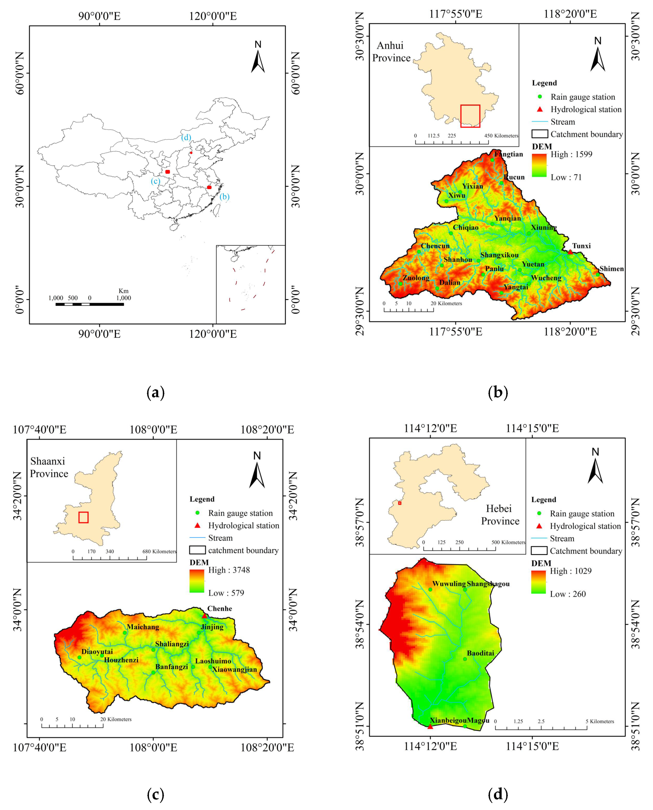
The study area for this research consisted of three catchments, i.e., Tunxi, Chenhe, and Xianbeigou, characterized as humid, semi-humid, and semi-arid regions, respectively (Figure 1).
The Tunxi Catchment is located in the southern part of Anhui Province in Eastern China (Figure 1b). Tunxi has typical mountainous terrain, i.e., high in the west and low in the east, with maximum, minimum, and average elevation of 1398 m, 116 m, and 380 m, respectively. It is a mesoscale catchment with a drainage area of 2670 km2 [37]. The average annual rainfall is approximately 1600 mm/year, of which more than 60% occurs between May and August due to the dominance of the monsoon climate. There is high annual and inter-annual variation in river runoff. Long-term rainfall data recorded per hour from 18 rain gauge stations as well as runoff data recorded at the outlet are available from the Hydrological Bureau of Anhui Province, China.
The Chenhe Catchment is situated in Shaanxi Province, and it is part of the Heihe River Basin, which has an area of 1350 km2 (Figure 1c). The annual precipitation is approximately 800 mm/year [38], and it varies significantly throughout the year, with massive rainstorms from July to October accounting for more than 60% of the mean annual precipitation. The average runoff depth ranges from 100 mm to 500 mm, and the runoff coefficient varies between 0.2 and 0.5. The watershed has one hydrological station and nine rainfall gauges. The recorded maximum flood discharge at Chenhe station was 1750 m3/s in 2005, and the minimum was 196 m3/s in 2004. The long-term hourly rainfall and runoff data were obtained from the Hydrological Bureau of Shaanxi Province, China.
The Xianbeigou Catchment is located in the arid area of Baoding City in Hebei Province (Figure 1d). The catchment has an area of 34.4 km2, and it is part of the Daqinghe River network in the Haihe River Basin. Long-term average precipitation is approximately 630 mm/year with maximum and minimum values of 1150 and 280 mm/year, respectively. The mean annual flow is approximately 226 million m3, with maximum and minimum values of 1390 and 200 million m3, respectively. The recorded maximum peak flow is 52.3 m3/s. The hydrograph is featured by steep rising and falling limbs. It should be emphasized that small watersheds in the northern and the northwestern mountainous areas of China have inadequate capacity for flood control and water retention and thus have high surface runoff and rapid hydrological response to rainfall events [39]. Flooding occurs between June and September as a result of uneven distribution and inter-annual variation in precipitation [40]. The long-term rainfall data from five rain gauges recorded at 20 min interval and runoff data recorded at the outlet are available from the Hydrological Bureau of Hebei Province, China.
The river networks of the three catchments (Figure 1) were derived from a digital elevation model (DEM) with a spatial resolution of 90 m. The DEM was provided by International Scientific and Technical Data Mirror Site, Computer Network Information Center, Chinese Academy of Sciences (http://datamirror.csdb.cn).
2.2. Data Preprocessing
The input variables were scaled to accelerate the convergence speed and make the training process faster [41] and were normalized using the following equation:
where and are the observed and the normalized runoff at time t, respectively.
Additionally, it should be noted that modeling boundary conditions were kept as similar as possible to allow comparison of different models. This means that input data, number of layers, number of neurons, dropout rate, and number of training epochs were kept identical. Therefore, each model acquired a different set of parameters with the same model structure, which showed the information from different catchments that could be analyzed based on simulation results. After training, the value was denormalized for comparison with observed data.
3. Methodology
3.1. LSTM Model
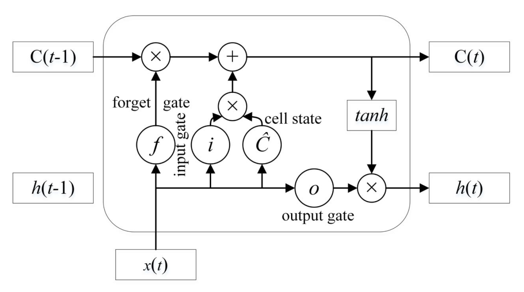
LSTM, proposed by Hochreiter and Schmidhuber [42], was an adapted version of RNN to address problems of exploding or vanishing gradient and later were refined or simplified [43]. This method can preserve information over long periods through its unique structure, cell state, and gates to control how the information flows in the different layers. The structure of the LSTM is shown in Figure 2. Equations are as follows:
where , and are the input gate, the forget gate, and the output gate, respectively; and represent the weights connecting input, forget, and output gates with the input, respectively; and denote the weights from input, forget, and output gates to the hidden states, respectively; and are input, forget, and output gate bias vectors, respectively; is the cell input; is the current cell state; refers to current hidden state; is the logistic sigmoidal function; is element-wise multiplication; and is the hyperbolic tangent function. The intuition behind this structure design is that the cell state acts as the memory unit to remember useful information through the different operations of each gate. The input gate filter is the information added to the cell with the assistance of current input and historical information, while the forget gate discards certain previous information, which allows the cell to clear the value it contains; subsequently, the output gate outputs the information selectively.
3.2. Xinanjiang Model
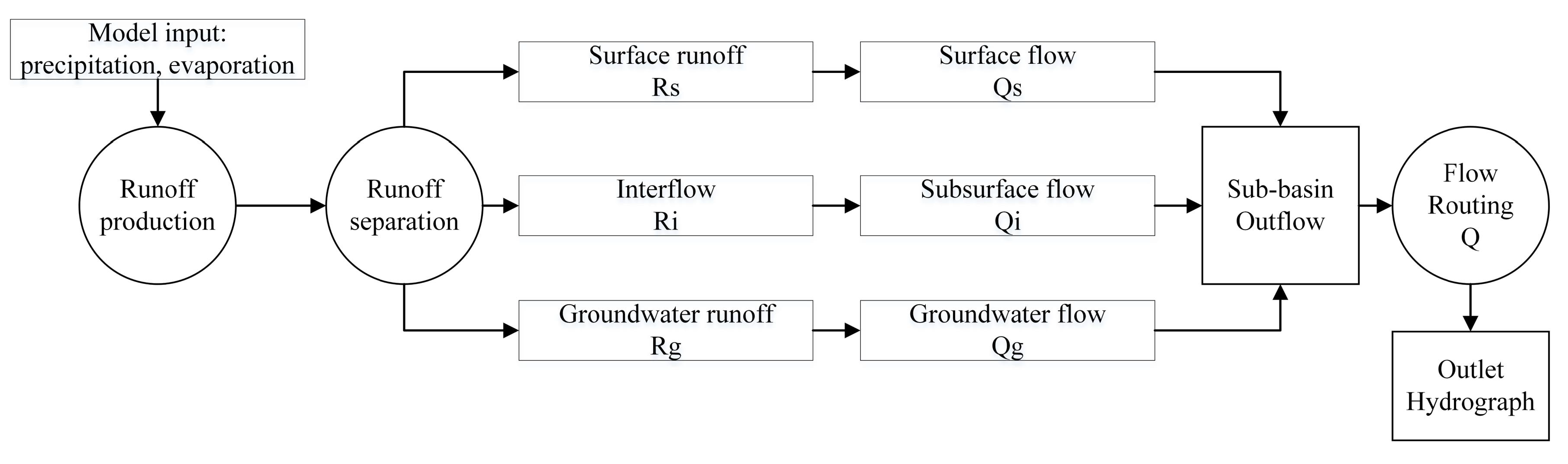
The XAJ model [44,45] is a conceptual rainfall–runoff model that has been successfully and widely used in humid and semi-humid regions of China. The flowchart of the XAJ model is shown in Figure 3 [46].
This model introduces the concept of runoff formation on the repletion of storage capacity in rainfall–runoff modeling and uses a parabola curve to depict the uneven storage distribution within the basin in a statistical manner [47]. The depth of the vadose zone is adopted to represent the water-holding capacity of the basin. The XAJ model mainly considers surface runoff and groundwater at first, and later it incorporates the concept of interflow introduced by hillslope hydrology as a sophisticated version that has been successfully and widely used for humid and semi-humid basins in China. The detailed description of the model can be found in Zhao [45]. The inputs for the XAJ model are rainfall and evaporation. The model transforms the input into surface, interflow, and groundwater components through runoff production calculation according to tension water storage and free water storage. In the second stage, the unit hydrograph or the lag routing technique are usually applied to conduct flow routing in the sub-basin. Finally, the runoff concentration of the channel system is represented by the Muskingum method [48], and then it outputs runoff at the target hydrological station. The dynamics of the water storage of the basin are reflected in the change of tension water variable W.
3.3. LSTM-KNN Model
The LSTM-KNN model incorporates the KNN algorithm into the model as an updating method for real-time forecasting. The KNN algorithm [49] is one of the non-parametric methods used for real-time updating in hydrological forecasting. Due to the temporal and the spatial similarity of flood events, similar underlying surface and weather conditions tend to generate parallel hydrographs [50]. Considering that KNN aims to learn from historical information similar to the current situation, it could be inferred that certain features from similar flood events could be used for error estimation when implementing this method.
In this study, KNN was applied to select the simulation error in each time step of the flood events; the Euclidean distance was chosen as the measurement of the proximity of input vectors to identify the most similar k hydrographs for estimating the simulation error using the k-nearest samples with the inverse-distance weighting method.
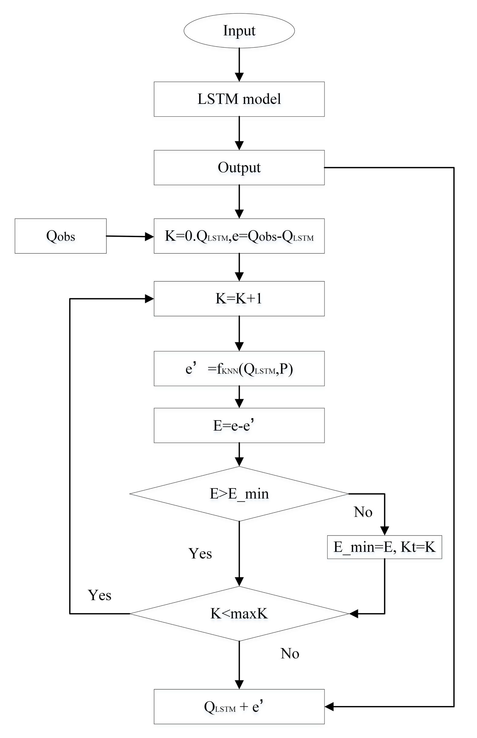
Figure 4 illustrates the flow chart for the implementation of the KNN algorithm in the hybrid model. The detailed description is as follows:
(1) Construction of a historical database. This was achieved by calculating simulation errors. After training of the LSTM model, we calculated the errors between the observed values and the LSTM simulation for the training set. In the KNN model, the relationship between the errors and the inputs is expressed by the equation below:
where denotes the simulation error at time , which is the difference between the LSTM results and the observed data. QLSTM,t-i is the result of the LSTM model at time , () is the vector that influences the discharge (such as precipitation) at time t-i, and is the dimension of the vector.
(2) Identification of the optimal number of k-nearest neighbors. The Euclidean distance was adopted to measure the distance between the inputs; all the vectors were sorted by the distance in ascending order to search k vectors that were the most similar to the inputs at time t.
(3) Estimation of errors. The weights of each historical error were calculated using the inverse distance weighted method as in Equation (9), and the errors at time t were determined by the weighted average of the number of k simulation errors.
(4) Updating the results. The error calculated by KNN was added to the results calculated by LSTM.
The K value was the only parameter that needed to be adjusted in the KNN algorithm and was optimized by the leave-one-out cross-validation method within the range [1,50]. The results of the LSTM model and the precipitation data were treated as the input for the KNN algorithm. The difference between the simulation error and the error calculated by KNN for each K was minimized to find the optimal K value, as depicted by Figure 4. Additionally, an LSTM-KNN model uses data more efficiently and thus may achieve a more stable performance, even with insufficient data, by leveraging from KNN’s capability to estimate errors from historical and newly collected information.
3.4. Model Framework
Our research is closely related to open-source software libraries. We developed the LSTM model described in Section 3.1 based on TensorFlow [51], an open-source software library provided by Google. The LSTM model constructed in this study includes one LSTM layer followed by a single fully connected layer, as recommended by some studies [14,52]. The results of the models mentioned above treat precipitation from the participating gauge stations as the only input in all three study regions. For Tunxi, eighteen flood events recorded from eighteen rain gauges between 2008−2016 were selected for training and testing processes, while fourteen flood events recorded from nine rain gauges between 2003−2012 for Chenhe catchment were selected. For the Xianbeigou catchment, the frequency of flooding was lower due to the semi-arid climate relative to the other two study regions. Therefore, ten flood events from five rain gauges from 1983 to 2007 were used. The LSTMs were run in sequence-to-sequence mode to predict the whole flood events with the precipitation data.
The main parameters of the LSTM neural network model were the weights and the biases, which were updated through the backpropagation through time algorithm (BPTT) [53]. Furthermore, the hyperparameters needed to be selected for the training procedure design. The proportion allocated to the training set was 70%, and the remainder was used as the testing set. The loss function was the mean squared error function. The number of hidden neurons of the LSTM layer was ten. The network was trained for 1000 epochs (where in one epoch, all the training samples were utilized for model optimization) to minimize the mean squared error using the adaptive moment estimation (Adam) optimization method [54] with an initial learning rate of 2e-3. Note that the models for different areas use the same hyperparameters.
Regularization was also used in training to avoid over-fitting and was achieved by adding penalty terms to the layer parameters (such as the weights) because large weights are often regarded as an indication of over-fitting. The penalty terms together with the loss function were the optimization objectives of the built neural network; the penalty coefficient was 1e-4. Equation (11) shows the loss function with L2 regularization.
3.5. Model Evaluation Criteria
The rooted mean square error (RMSE), the Nash-Sutcliffe efficiency (NSE) coefficient, the R-squared score (R2), and the volume error (VE) were adopted to evaluate the model accuracy.
RMSE evaluates the proximity of the predicted values to the observed values based on the relative range of the data. In general, a lower RMSE suggests higher accuracy.
The NSE is a frequently used index to evaluate the performance of hydrological models. It gives a measurement of model ability to predict variables different from the mean and gives the proportion of the initial variance accounted for by the model [55], ranging from minus infinity to 1; a value approximating to 1 means that the simulated process is close to observed values.
R2 is the square of the sample correlation coefficient ranging from 0 to 1, and it evaluates the amount of model variance.
The VE shows the accuracy of the flood volume, which is an index to evaluate the model performance for measuring water balance, where a value close to 0 suggests the simulation is close to the observed data.
4. Results
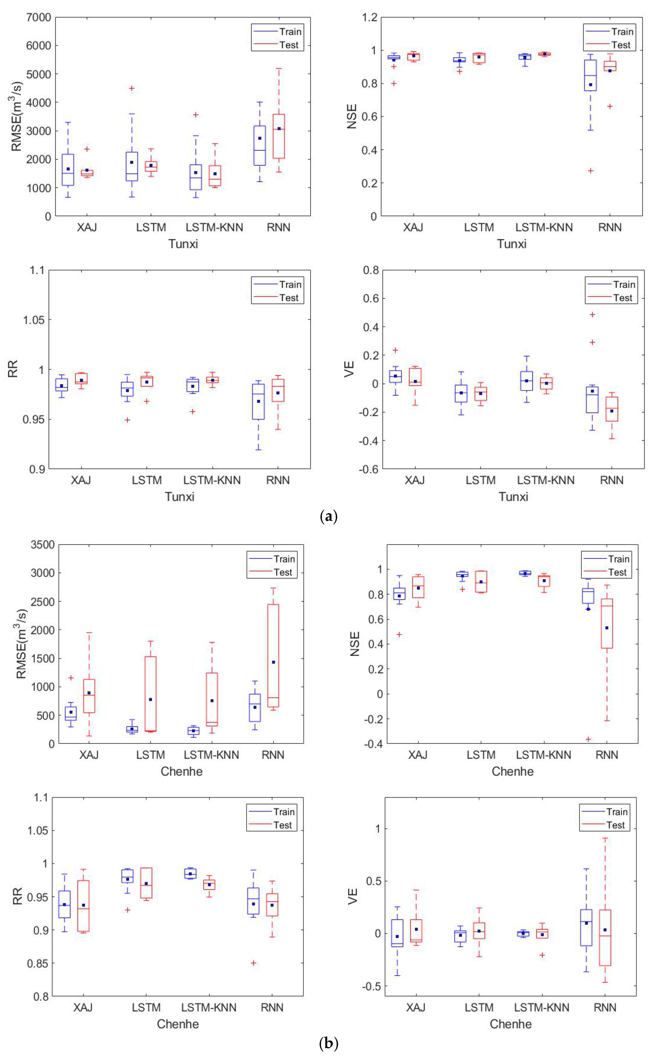
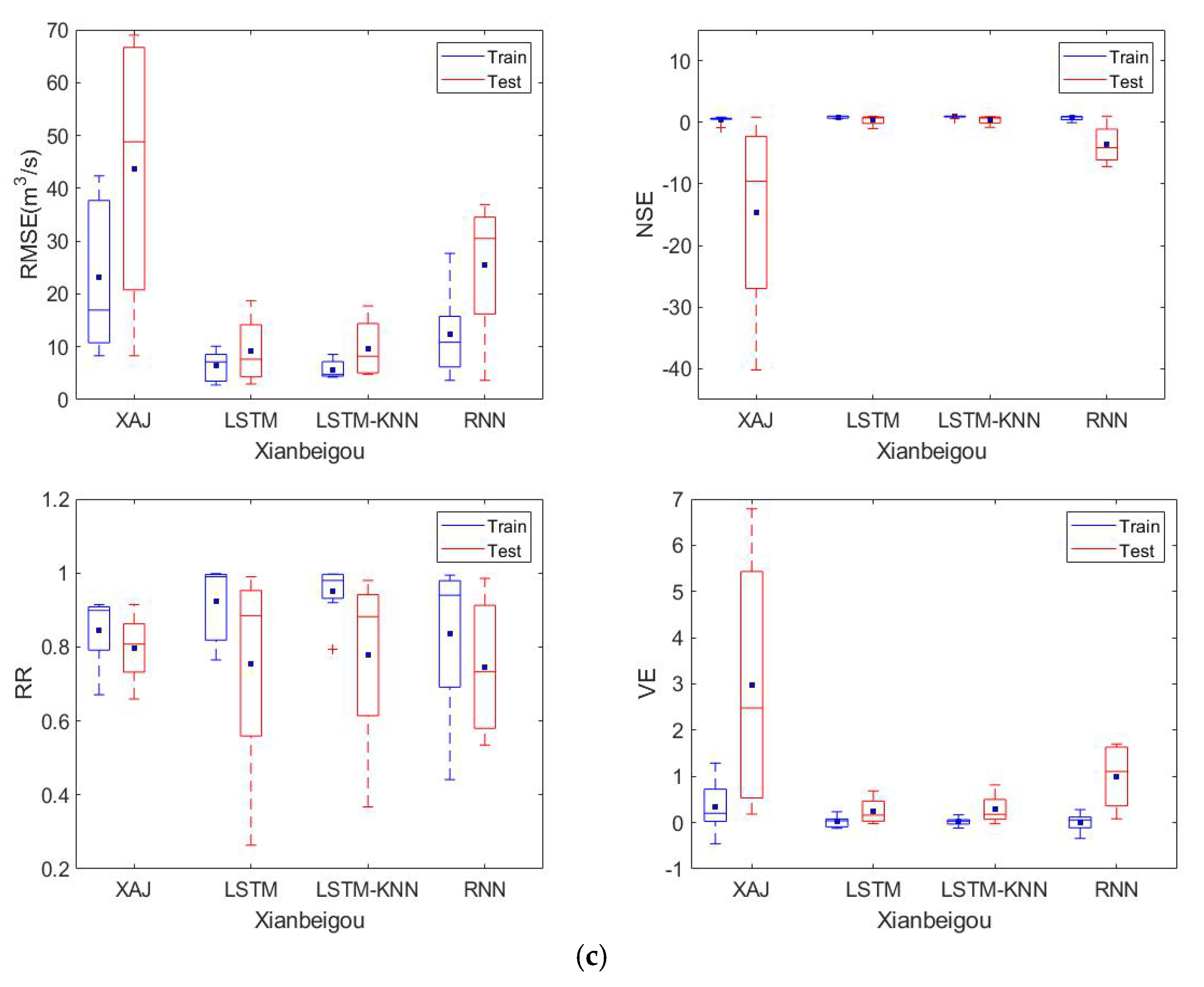
First, the performance of LSTM and RNN models are evaluated in Section 4.1. In Section 4.2, the LSTM model is compared with the XAJ model to explore the similarities of these two models. Finally, in Section 4.3, we discuss the effectiveness of the proposed LSTM-KNN model relative to the LSTM model. Results in terms of the four evaluation metrics in all study areas for the testing and the training set are summarized in Table 1. The boxplots of the statistics of RMSE, NSE, R2, and VE for each flood event in the three study catchments for training and testing are displayed in Figure 5.
4.1. Comparison between RNN and LSTM Models
As seen in Table 1, the values of each LSTM metric were improved compared to those of the RNN model in each basin for both training and testing data. The NSE values of LSTM for training generally ranged between 0.85 and 0.93, and for the testing period, they varied from 0.33 to 0.96. In addition, the RMSE of LSTM was much smaller than that of RNN with the RMSE ranging from 9.24 m3/s from 1786 m3/s for validation. Both models showed relatively high R2 values, while LSTM showed higher values than RNN for training and testing samples. The improvements for VE were also evident in these study regions. The mean VE values of LSTM were smaller than those of RNN, which implies that the simulated flood volume of LSTM was close to observed values. This finding suggests that LSTM could produce the hydrograph with a reasonably high water balance accuracy.
The boxplots indicate NSE, RMSE, RR, and VE of each modeled flood event for both training and testing samples and each of the three catchments. Similar conclusions as in Table 1 could be drawn from Figure 5. It can be observed that the box for RNN had a broader distribution than that of the LSTM model. The graphical results (Figure 5) reveal that the discharge simulations from the LSTM model were close to the observations; thus, it is capable of computing both the hydrograph and the peak flow.
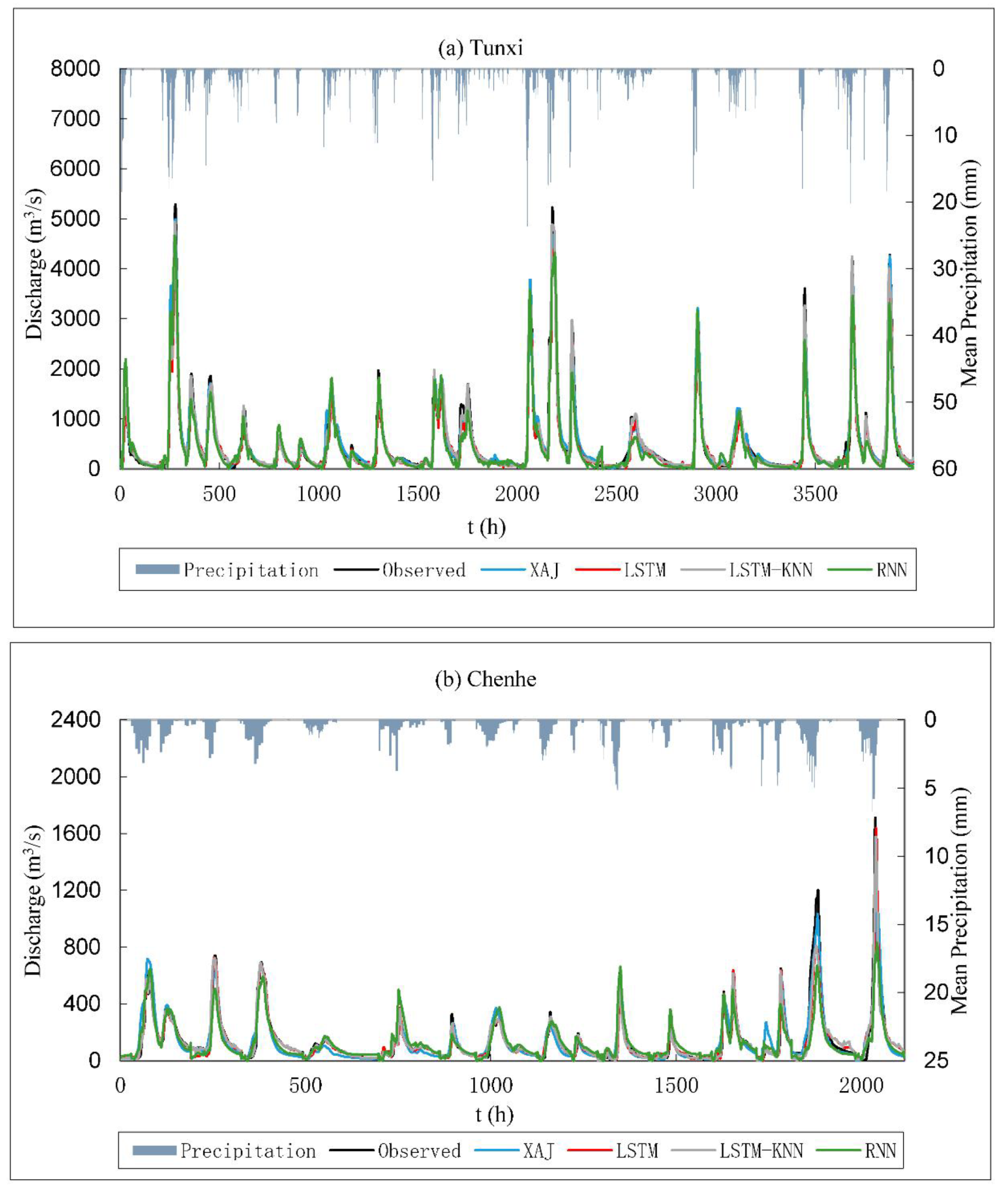
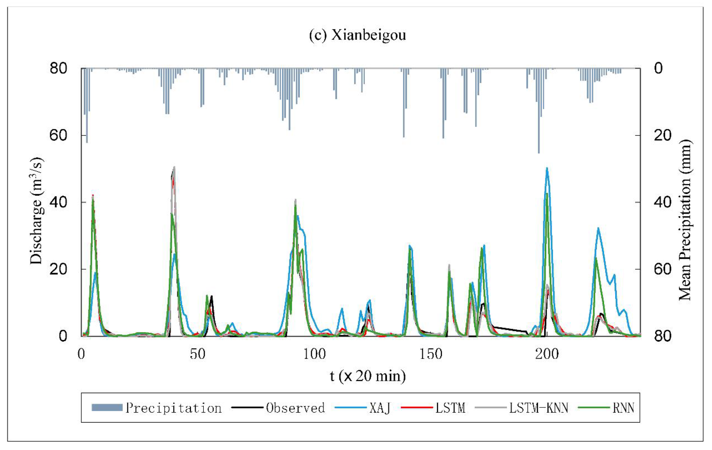
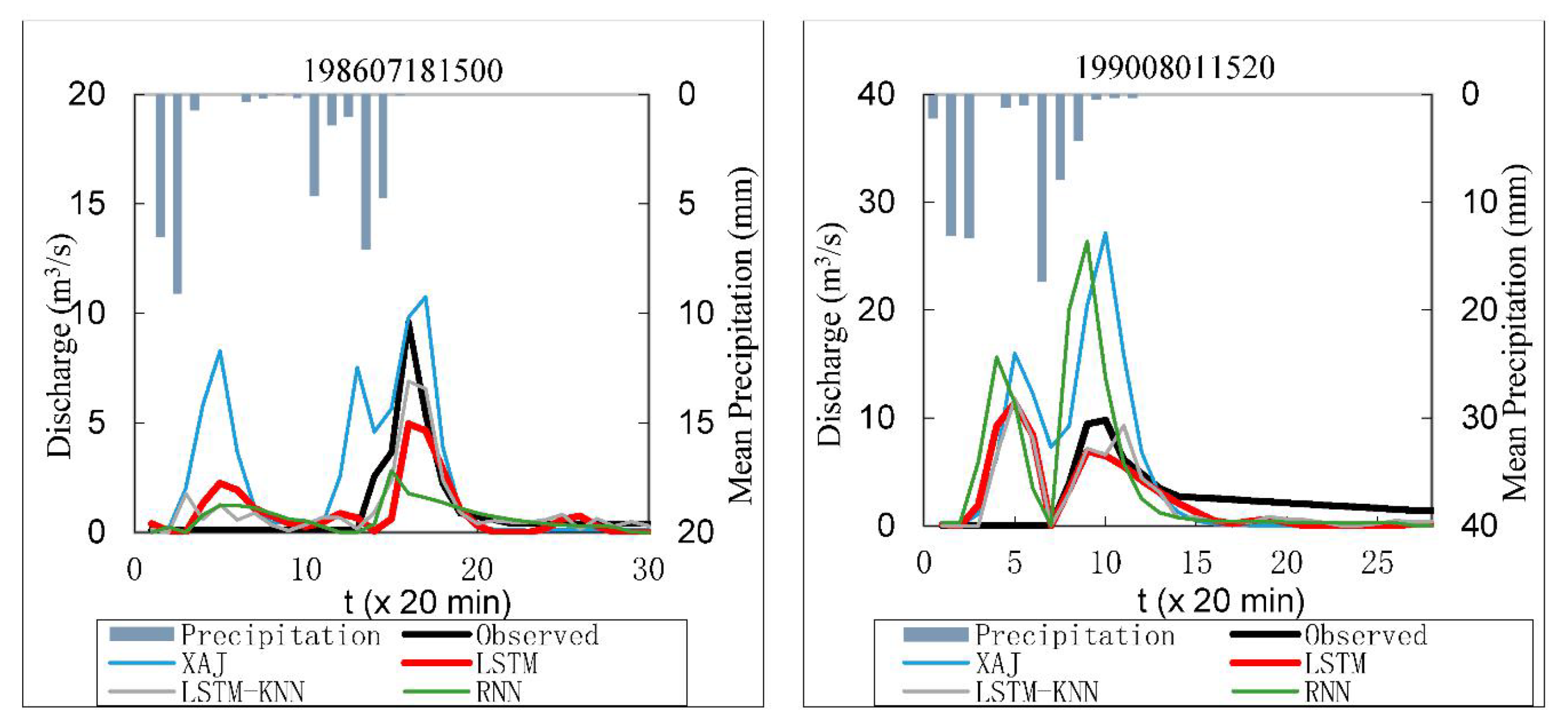
For the model performance in individual catchments, the results varied significantly. The LSTM model could give more accurate simulation in Tunxi, but the results given by RNN suggest inevitable fluctuations (Figure 6). In Chenhe Catchment, the LSTM model tended to underestimate the discharge relative to the observations, as precipitation was derived by interpolation to compensate for missing hourly rainfall in specific periods. This led to smaller inputs in flood peak periods for certain flood events. All the model performances were not entirely satisfactory owing to the limited flood sample size compared with the other two catchments. RNN often overestimated or underestimated the flood volume in Xianbeigou. The simulations from the testing sample using the LSTM model showed much lower flood peak errors than the RNN model, while the LSTM did not perform satisfactorily; i.e., the value of NSE was 0.33 in the testing stage. The unsatisfactory performance was due to limited sample size, i.e., seven flood events for training and three flood events for testing were used for Xianbeigou catchment. The NSE value of 0.85 in the training stage implies some degree of over-fitting. Furthermore, the data quality adds more difficulties for accurate simulation. Figure 7 shows the hydrographs of the flood events #198607181500 (a training sample) and #199008011520 (a testing sample), indicating that data quality may be a problem. Xianbeigou has a relatively small drainage area, i.e., 34.4 km2. It is generally acknowledged that such a catchment should be sensitive to high-intensity rainfall and the discharge will quickly respond to rainfall. However, in Figure 7, it is clear that the LSTM model calculated fit this description, while there was no rising limb after the first peak of the precipitation in the observed discharge series.
It is clear that the predicted hydrograph using the LSTM model showed a smoother pattern and fit well with the general trend of the hydrograph (Figure 6), while the RNN model showed some oscillations in the simulated results. Considering that the RNN and the LSTM input were the same, the results might imply the impact of the structural difference on the simulation. The results suggest that the structure of LSTM enables a better illustration of the hydrological processes because the additional cell state of the LSTM model provides a way to mimic the storage ability of the catchments.
4.2. Comparison between XAJ and LSTM Models
The simulations from both XAJ and LSTM models showed better goodness-of-fit in Tunxi. The NSE performance of the LSTM model in the training stage was 0.93 compared to 0.94 achieved by the XAJ model; on the other hand, they attained an equal value of 0.96 during the testing stage. The same values were obtained for R2. The other two evaluation criteria differed markedly. The performance of the LSTM model was not as good as the XAJ model in this catchment. Overall, the XAJ model had much better performance relative to the LSTM model in Tunxi because the XAJ model was first developed in the Xinanjiang Basin, of which Tunxi is part of, and it is a typical humid basin with a highly linear rainfall–runoff relationship as flood events with high peak flows regularly occur. The structure was well designed, and the parameterization was fully investigated according to the characteristics in that basin [47]. On the other hand, the LSTM model did not achieve better results than the XAJ model; both XAJ and LSTM models produced satisfactory results. Thus, we could conclude that LSTM demonstrates a relatively strong capability to capture the rainfall–runoff relationship for flood events in humid regions.
In the Chenhe Catchment, the results were entirely different from those in Tunxi. As it can be seen in Figure 5, the performance of each evaluation index decreased compared with the application in Tunxi using the XAJ model. The LSTM model had a narrower range of RMSE between 267 m3/s and 778 m3/s relative to the XAJ model. The value of NSE was also improved from 0.80 (XAJ) to 0.90 (LSTM) in the training stage, while for validation, it rose from 0.85 to 0.95 accordingly. The R2 value increased from 0.94 to 0.97 for both training and testing sets. The volume error decreased from 17.32% for XAJ to 0.87% for LSTM in the training stage and dropped from 3.22% for XAJ to 2.00% for LSTM in the testing stage. The LSTM model yielded better results compared with the XAJ model in Chenhe because the catchment possesses a semi-humid climate, and the water resources are less abundant compared with Tunxi. Furthermore, the infiltration–excess runoff mechanism may exist in this area [38]. Therefore, the XAJ model, which is based on a saturation–excess runoff generation mechanism, might not be able to generate comparable results in Chenhe compared to Tunxi, while LSTM could better learn the characteristics of this catchment.
In Xianbeigou, the volume error of LSTM was less than that of XAJ, and the shape of the simulated hydrograph of LSTM closely matched the observed data. However, the LSTM performance of the other three metrics in the training stage was better than in the testing stage. To some extent, this might be a sign of over-fitting or could have been due to the small magnitude of the discharge in this catchment that exaggerated the error. Overall, the small flood events imparted significant uncertainty to the parameterization of the XAJ model, which may have been partially responsible for the deficits in the model simulation. Furthermore, infiltration–excess runoff was the dominant runoff generation mechanism leading to rainfall-triggered floods with short duration and fast recession. It is, therefore, not suitable to apply the XAJ model with saturation–excess runoff generation mechanisms in this watershed characterized by sharply rising and falling flows. However, the LSTM model yielded better results than the XAJ model for both training and testing. This finding indicates LSTM’s robustness to small data samples and its potential applicability in other similar types of catchments. However, poor testing stage performance is concerning.
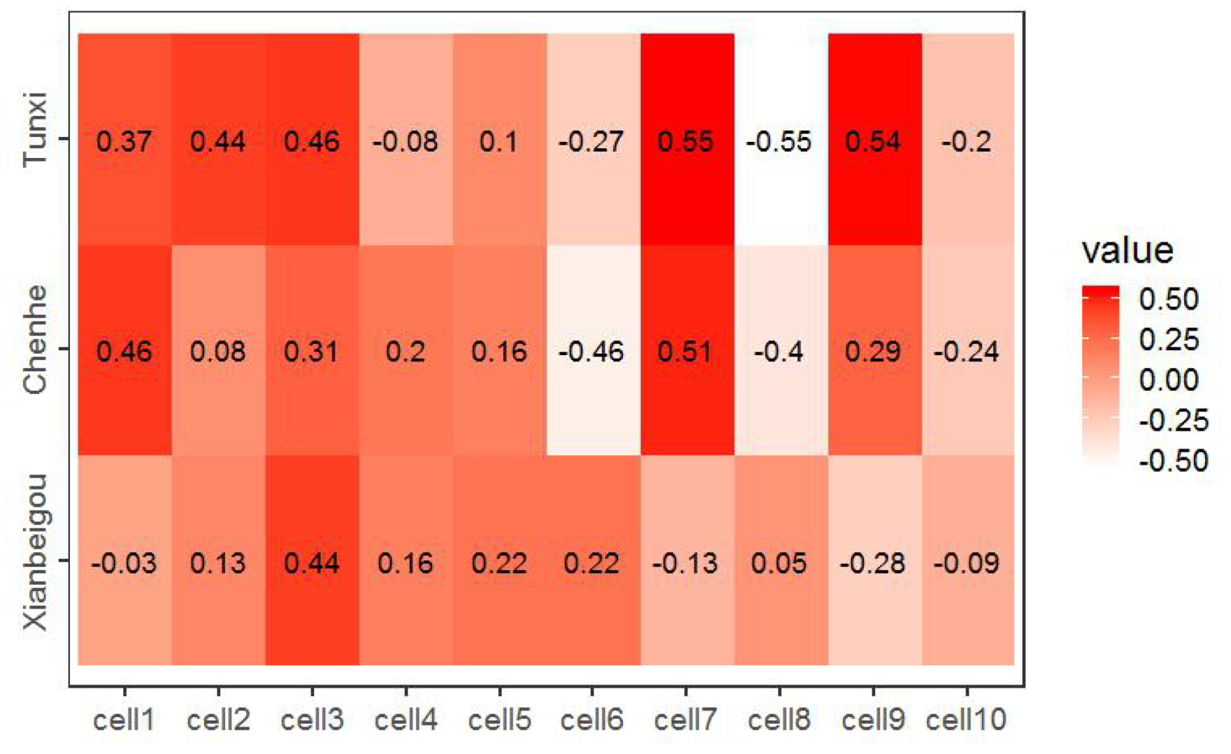
Frederik [56] proposed that the correlation between the LSTM model and the conceptual model could be calculated to see if there is a strong relationship between the cell values of LSTM and states variables of other hydrological models. Similarly, we extracted the cell states of LSTM and the tension water W representing the soil moisture in the XAJ model. Considering that the input in the LSTM model was normalized to be fed into the model, the absolute value did not contain physical meaning. Therefore, the correlation of these two variables could be examined to ascertain if the cell states had the same function as the state variable W from the XAJ model.
Figure 8 shows the average correlation of every memory cell with the hydrological states considered in this experiment. The positive correlation values for Tunxi, Chenhe, and Xianbeigou were six, seven, and six, respectively. Tunxi Catchment contained the most cells that correlated the W of XAJ model with more significant values, followed by Chenhe. Both catchments had more cells with a relatively higher correlation than Xianbeigou. This finding is consistent with the above simulation results, since the complexity of simulating the rainfall–runoff relationship in these three basins is also arranged in that order. Additionally, the sample size might have contributed to this phenomenon. It should be noted that Tunxi had the most considerable quantity of training samples among these study regions, while the flood sample size of Xianbeigou was the smallest. As a result, the larger sample size enabled a more objective training procedure because various conditions were fully considered during the optimization. Additionally, the XAJ model did not achieve the desired results in Xianbeigou; thus, the relatively weak correlation for the Xianbeigou watershed was also reasonable. Furthermore, in the semi-arid and the arid regions in China, the runoff generation is dominated by the infiltration runoff process. This mechanism has a high relation to precipitation intensity. Thus, we inferred that this relationship is complicated for the cell to learn since this process is represented by the comparison of the precipitation intensity and the infiltration capacity of the soil. While this kind of information is not included in the current model input, it may be challenging for the model to extract the information. Therefore, as both the data quantity and the runoff generation mechanism are intertwined, poor model performance was seen in semi-arid regions.
Overall, in all three catchments, some of the memory cells had a particularly high correlation with the provided hydrological states, which shows that the cell might have acted as a reservoir with a certain amount of storage to adjust the runoff process in the catchment.
4.3. Comparison of LSTM, LSTM-KNN Model
The leave-one-out cross-validation method for optimization resulted in K of 14, eight, and three for Tunxi, Chenhe, and Xianbeigou, respectively. The difference in K for each basin is related to the differences in sample size, as more samples provided KNN with more references to calculate the error. Tunxi had the largest sample size, followed by Chenhe, while Xianbeigou catchment had the smallest sample size.
Table 1 lists the evaluation metrics of the updated results for the coupled model. The performance of the LSTM-KNN was better than that of the single LSTM model for the four evaluation metrics, which means that the updated simulations were superior to the original simulation. The RMSE decreased from 260 m3/s to 218 m3/s for the training sample. The value of NSE obtained from the LSTM-KNN model was higher than 0.93 and 0.96 for the training and the testing stages, respectively, for Tunxi. Similar results could be witnessed in the other two catchments. R2 values remained the same for Tunxi, while a slight increase from 0.97 to 0.98 was witnessed in the training sets for Chenhe catchment. This improvement was evident in Xianbeigou catchment. The volume error had a trend close to zero when applying the KNN method in all the basins. In Figure 5, the four indexes of LSTM were distributed in a marginally more extensive range than that of the coupled model, especially for Tunxi and Chenhe. Therefore, the LSTM-KNN model promoted the LSTM model performance in all three watersheds. Our results show that the LSTM-KNN model yielded relatively better performance in all three catchments, which demonstrates that the KNN algorithm, acting as an error updating model, could select useful historical data points that effectively reduced the error accumulation.
5. Discussion
We compared and discussed the performance of the four models in selected catchments. In comparison to previous studies in the humid catchment, i.e., Tunxi, Yao [37] found NSE of 0.94 (i.e., for training sample) and 0.95 (i.e., for testing sample) from XAJ and improved Xinanjiang coupled with geomorphologic instantaneous unit hydrograph (XAJ-GIUH) models using time series data from 1983 to 2003. However, we found higher accuracy with NSE of 0.96 (i.e., for training sample) and 0.98 (i.e., for testing sample) from the LSTM-KNN model using data spanning from 2008 to 2016. Huo [38] classified the flood events in Chenhe catchment in the same period as this study into low-flow, medium-flow, and high-flow events and utilized six hydrological models to simulate the flood events while applying the Bayesian model averaging (BMA) approach to improve flood prediction. The NSE value of the selected flood events for testing sample was 0.86. In comparison, our LSTM model showed better model prediction ability in Chenhe with an NSE of 0.93 for the testing stage, which suggests the superiority of the LSTM model. In another study, Chao [39] established the CASCade Two Dimensional SEDiment (CASC2D-SED) model in Xianbeigou Catchment; the coefficient of determination (i.e., a similar metric with NSE) of eight flood events was greater than 0.7 with an average of 0.85, and the accuracy of simulation results was higher than that of LSTM found in this study. This is because the CASC2D-SED model utilizes the Greet-Ampt formula to simulate surface flow, which is suitable for this area with steep hydrographs that show the infiltration–excess mechanism.
However, it is noteworthy that the LSTM model achieves better results in semi-arid regions, which suggests that the data-driven model can acquire a more reliable system pattern than the XAJ model. On the contrary, the structure design of the XAJ model is based on the saturation–excess runoff generation mechanism, while the runoff generation mechanism in semi-arid or arid basins is dominated by infiltration–excess runoff. Therefore, it is challenging to produce a simulation with high accuracy using the conceptual XAJ model due to the lack of sufficient description of the mechanisms in semi-arid or arid basins. The XAJ model utilizes water balance mechanisms in its design structure, while the extensive impact of human activity on natural basins and intensified groundwater resources dependence in most semi-arid basins in China might render this hypothesis inapplicable [57]. As suggested in Section 4.3, poor data quality and quantity are the main issues. The accuracy of flood forecasting relies heavily on data availability in the relative dry watersheds. In these areas, the rainfall has an uneven spatial distribution, and the time interval is sparse, occasionally capturing the peaks in flash floods with the rapid rise and fast recession. As a result, high-density precipitation data are the primary requirement for producing reliable simulation. In reality, this requirement is often difficult to meet in some watersheds due to spatial and temporal variability of rainfall and the lack of observations. Therefore, more research needs to be done in the future to tackle these problems, possibly with the incorporation of radar or satellite precipitation products [58]. On the other hand, probabilistic forecasting, such as the Bayesian inference method, is also an alternative considering that more uncertainties could be taken into account during the modeling [59].
Furthermore, using confined forcing such as meteorological forcing data to derive LSTM models shows good potential for further integration of LSTM-based models into the operational settings driven by precipitation data obtained from weather radar. However, other static catchment characteristics could also be introduced in the LSTM model as inputs, such as the topography and the vegetation [2,60], due to their vital role in the runoff generation and the routing process in rainfall–runoff modeling. Therefore, incorporating more catchment attributes in the LSTM model would further enhance its capability for streamflow forecasting.
In regions with intense human activity, the regulation and the management of dams, reservoirs, and other hydraulic projects are crucial to reducing the loss of life and property caused by flood disasters. These hydraulic projects are generally treated as internal nodes in conventional hydrological models for better use and planning. Although LSTM could provide high accuracy forecasting, it could only give the simulation or the forecast at the target hydrological station or specific cross-section of the river channel. Moreover, the fact that the LSTM internal variables cannot be directly interpreted or reflect the internal dynamics of the catchment is a challenge that impedes its full application. Therefore, combining LSTM with other hydrological or hydraulic models for flood warning or other water use purposes is another viable option for future research, such as incorporating other hydraulic models for river channel flow routing to obtain detailed information at each important cross-section.
Real-time flood forecasting is a critical tool in the operational flood emergency management system. The updating or the data assimilation techniques could account for the inaccuracy of input data, state variables, model parameters, and output variables [31]. The most widely used procedure in operational flood forecasting is output variable updates, such as the autoregressive model [61]. Our study mainly considers the errors of the output variables by utilizing the simulation results of LSTM and the precipitation as the inputs of KNN regression methods. Other techniques that are not aiming at the correction of the outputs could also be employed in real-time flood forecasting, such as utilizing the Kalman filter to realize the optimal estimation of the system state variables [62].
6. Conclusions
This research investigated the application of the LSTM model in flood forecasting. Meanwhile, the applicability of LSTM-KNN models for operational streamflow forecasting systems was explored. Three study regions in China with different climate conditions (humid, semi-humid, and semi-arid) were selected to test the efficiency of the proposed models. The model results were compared with one of the artificial intelligence techniques, RNN. Additionally, the conceptual-based XAJ model was constructed to detect the similarities between the conceptual model and the data-driven model. Finally, a coupled LSTM-KNN model was proposed to see if it had the potential to be generalized in the application of real-time forecasting.
The results prove that the LSTM with internal memory has the ability to learn and store long-term dependencies of the input–output relationship in different climates. LSTM could produce comparable results as the conceptual XAJ model, and the results exhibit that it obtains more robust results compared with the simple RNN model. The comparisons between the coupled model and the LSTM model also show that the KNN algorithm could increase the accuracy of the LSTM model in predicting runoff in three catchments. Therefore, it would be a more suitable approach to improve the accuracy in the context of real-time runoff forecasting.
Author Contributions
Conceptualization, M.L., Y.H., Z.L. (Zhentao Liu) and F.J.; Data curation, M.L.; Formal analysis, M.L. and Z.L. (Zhentao Liu); Funding acquisition, Y.H. and Z.L. (Zhijia Li); Methodology, M.L. and Z.L. (Zhentao Liu); Project administration, Y.H. and Z.L. (Zhijia Li); Resources, Z.L. (Zhijia Li) and M.S.; Software, M.L. and Y.H.; Supervision, Z.L. (Zhijia Li); Validation, B.T.; Visualization, M.L., B.T., M.S. and H.Z.; Writing–original draft, M.L.; Writing–review & editing, Y.H., B.T., Z.L. (Zhentao Liu), F.J. and H.Z. All authors have read and agreed to the published version of the manuscript.
Funding
This work was supported by the National Key R&D Program of China (Grant No. 2018YFC1508102, Grant No. 2016YFC0402705), the National Natural Science Foundation of China (Grant No. 51679061, Grant No. 51909059), the Natural Science Foundation of Jiangsu Province (Grant No. BK20190492), and the Fundamental Research Funds for the Central Universities (Grant No. 2016B04714).
Conflicts of Interest
The authors declare no conflict of interests regarding the publication of this paper.
References
- Jeong, J.; Park, E. Comparative applications of data-driven models representing water table fluctuations. J. Hydrol. 2019, 572, 261–273. [Google Scholar] [CrossRef]
- Kratzert, F.; Klotz, D.; Shalev, G.; Klambauer, G.; Hochreiter, S.; Nearing, G. Benchmarking a Catchment-Aware Long Short-Term Memory Network (LSTM) for Large-Scale Hydrological Modeling. Hydrol. Earth Syst. Sci. Discuss. 2019, 2019, 1–32. [Google Scholar]
- Abrahart, R.J.; See, L.M.; Solomatine, D.P. (Eds.) Data-Driven Modelling: Concepts, Approaches and Experiences. In Practical Hydroinformatics: Computational Intelligence and Technological Developments in Water Applications; Springer: Berlin/Heidelberg, Germany, 2008; pp. 17–30. [Google Scholar]
- Sivapalan, M.; Takeuchi, K.; Franks, S.W.; Gupta, V.K.; Karambiri, H.; Lakshmi, V.; Liang, X.; McDonnell, J.J.; Mendiondo, E.M.; O’Connell, P.E.; et al. IAHS Decade on Predictions in Ungauged Basins (PUB), 2003–2012: Shaping an exciting future for the hydrological sciences. Hydrol. Sci. J. 2003, 48, 857–880. [Google Scholar] [CrossRef] [Green Version]
- Kratzert, F.; Klotz, D.; Brenner, C.; Schulz, K.; Herrnegger, M. Rainfall–runoff modelling using Long Short-Term Memory (LSTM) networks. Hydrol. Earth Syst. Sci. 2018, 22, 6005–6022. [Google Scholar] [CrossRef] [Green Version]
- Hsu, K.; Gupta, H.V.; Sorooshian, S. Artificial Neural Network Modeling of the Rainfall-Runoff Process. Water Resour. Res. 1995, 31, 2517–2530. [Google Scholar] [CrossRef]
- Seo, Y.; Kim, S.; Kisi, O.; Singh, V.P. Daily water level forecasting using wavelet decomposition and artificial intelligence techniques. J. Hydrol. 2015, 520, 224–243. [Google Scholar] [CrossRef]
- Chang, F.; Tsai, Y.; Chen, P.; Coynel, A.; Vachaud, G. Modeling water quality in an urban river using hydrological factors – Data driven approaches. J. Environ. Manag. 2015, 151, 87–96. [Google Scholar] [CrossRef] [PubMed]
- Alizadeh, Z.; Yazdi, J.; Kim, H.J.; Al-Shamiri, K.A. Assessment of Machine Learning Techniques for Monthly Flow Prediction. Water 2018, 10, 1676. [Google Scholar] [CrossRef] [Green Version]
- Akbari Asanjan, A.; Yang, T.; Hsu, K.; Sorooshian, S.; Lin, J.; Peng, Q. Short-Term Precipitation Forecast Based on the PERSIANN System and LSTM Recurrent Neural Networks. JGR Atmos. 2018, 123, 12543–12563. [Google Scholar] [CrossRef]
- Shen, C.; Laloy, E.; Elshorbagy, A.; Albert, A.; Bales, J.; Chang, F.; Ganguly, S.; Hsu, K.L.; Kifer, D.; Fang, Z.; et al. HESS Opinions: Incubating deep-learning-powered hydrologic science advances as a community. Hydrol. Earth Syst. Sci. 2018, 11, 5639–5656. [Google Scholar] [CrossRef] [Green Version]
- Lecun, Y.; Bengio, Y.; Hinton, G. Deep learning. Nature 2015, 521, 436. [Google Scholar] [CrossRef] [PubMed]
- Shen, C. A Transdisciplinary Review of Deep Learning Research and Its Relevance for Water Resources Scientists. Water Resour. Res. 2018, 54, 8558–8593. [Google Scholar] [CrossRef]
- Zhang, J.; Zhu, Y.; Zhang, X.; Ye, M.; Yang, J. Developing a Long Short-Term Memory (LSTM) based model for predicting water table depth in agricultural areas. J. Hydrol. 2018, 561, 918–929. [Google Scholar] [CrossRef]
- Hu, C.; Wu, Q.; Li, H.; Jian, S.; Li, N.; Lou, Z. Deep Learning with a Long Short-Term Memory Networks Approach for Rainfall-Runoff Simulation. Water 2018, 10, 1543. [Google Scholar] [CrossRef] [Green Version]
- Zhang, D.; Peng, Q.; Lin, J.; Wang, D.; Liu, X.; Zhuang, J. Simulating Reservoir Operation Using a Recurrent Neural Network Algorithm. Water 2019, 11, 865. [Google Scholar] [CrossRef] [Green Version]
- Fang, K.; Shen, C.; Kifer, D.; Yang, X. Prolongation of SMAP to Spatiotemporally Seamless Coverage of Continental U.S. Using a Deep Learning Neural Network. Geophys. Res. Lett. 2017, 44, 11–030. [Google Scholar] [CrossRef] [Green Version]
- Yuan, X.; Chen, C.; Lei, X.; YuanRana, Y.; Adnan, M. Monthly runoff forecasting based on LSTM–ALO model. Stoch. Environ. Res. Risk Assess. 2018, 32, 2199–2212. [Google Scholar] [CrossRef]
- Wu, Y.; Liu, Z.; Xu, W.; Feng, J.; Palaiahnakote, S.; Lu, T. Context-Aware Attention LSTM Network for Flood Prediction. In Proceedings of the 2018 24th International Conference on Pattern Recognition (ICPR), Beijing, China, 20–24 August 2018. [Google Scholar]
- Feng, J.; Yan, L.; Hang, T. Stream-Flow Forecasting Based on Dynamic Spatio-Temporal Attention. IEEE Access. 2019, 7, 134754–134762. [Google Scholar] [CrossRef]
- Längkvist, M.; Karlsson, L.; Loutfi, A. A review of unsupervised feature learning and deep learning for time-series modeling. Pattern Recogn. Lett. 2014, 42, 11–24. [Google Scholar] [CrossRef] [Green Version]
- Bengio, Y.; Courville, A.; Vincent, P. Unsupervised feature learning and deep learning: A review and new perspectives. IEEE Trans. Pattern Anal. Mach. Intell. 2013, 35, 1798–1828. [Google Scholar] [CrossRef]
- Maier, H.R.; Jain, A.; Dandy, G.C.; Sudheer, K.P. Methods used for the development of neural networks for the prediction of water resource variables in river systems: Current status and future directions. Environ. Modell. Softw. 2010, 25, 891–909. [Google Scholar] [CrossRef]
- Wu, C.L.; Chau, K.W.; Li, Y.S. Predicting monthly streamflow using data-driven models coupled with data-preprocessing techniques. Water Resour. Res. 2009, 45. [Google Scholar] [CrossRef] [Green Version]
- Zhang, X.; Zhang, Q.; Zhang, G.; Nie, Z.; Gui, Z.; Que, H. A Novel Hybrid Data-Driven Model for Daily Land Surface Temperature Forecasting Using Long Short-Term Memory Neural Network Based on Ensemble Empirical Mode Decomposition. Int. J. Environ. Res. Public Health 2018, 15, 1032. [Google Scholar] [CrossRef] [PubMed] [Green Version]
- Wang, L.; Li, X.; Ma, C.; Bai, Y. Improving the prediction accuracy of monthly streamflow using a data-driven model based on a double-processing strategy. J. Hydrol. 2019, 573, 733–745. [Google Scholar] [CrossRef]
- Liu, Y.; Weerts, A.H.; Clark, M.; Hendricks Franssen, H.J.; Kumar, S.; Moradkhani, H.; Seo, D.J.; Schwanenberg, D.; Smith, P.; van Dijk, A.I.J.M.; et al. Advancing data assimilation in operational hydrologic forecasting: Progresses, challenges, and emerging opportunities. Hydrol. Earth Syst. Sci. 2012, 16, 3863–3887. [Google Scholar] [CrossRef] [Green Version]
- Brajard, J.; Carrassi, A.; Bocquet, M.; Bertino, L. Combining data assimilation and machine learning to emulate a dynamical model from sparse and noisy observations: A case study with the Lorenz 96 model. Geosci. Model Dev. Discuss. 2019, 2019, 1–21. [Google Scholar] [CrossRef] [Green Version]
- Wan, X.; Yang, Q.; Jiang, P.; Zhong, P.A. A Hybrid Model for Real-Time Probabilistic Flood Forecasting Using Elman Neural Network with Heterogeneity of Error Distributions. Water Resour. Manag. 2019, 33, 4027–4050. [Google Scholar] [CrossRef]
- Ren, J.; Ren, B.; Zhang, Q.; Zheng, X. A Novel Hybrid Extreme Learning Machine Approach Improved by K Nearest Neighbor Method and Fireworks Algorithm for Flood Forecasting in Medium and Small Watershed of Loess Region. Water 2019, 11, 1848. [Google Scholar] [CrossRef] [Green Version]
- Liu, K.; Yao, C.; Chen, J.; Li, Z.; Li, Q.; Sun, L. Comparison of three updating models for real time forecasting: A case study of flood forecasting at the middle reaches of the Huai River in East China. Stoch. Environ. Res. Risk Assess. 2017, 31, 1471–1484. [Google Scholar] [CrossRef]
- Karlsson, M.; Yakowitz, S. Nearest-neighbor methods for nonparametric rainfall-runoff forecasting. Water Resour. Res. 1987, 23, 1300–1308. [Google Scholar] [CrossRef]
- Shamseldin, A.Y.; O’Connor, K.M. A nearest neighbour linear perturbation model for river flow forecasting. J. Hydrol. 1996, 179, 353–375. [Google Scholar] [CrossRef]
- Kan, G.; He, X.; Ding, L.; Li, J.; Lei, T.; Liang, K.; Hong, Y. An improved hybrid data-driven model and its application in daily rainfall-runoff simulation. IOP Conf. Ser. Earth Environ. Sci. 2016, 46, 12029. [Google Scholar] [CrossRef] [Green Version]
- Kan, G.; Li, J.; Zhang, X.; Ding, L.; He, X.; Liang, K.; Jiang, X.; Ren, M.; Li, H.; Wang, F.; et al. A new hybrid data-driven model for event-based rainfall–runoff simulation. Neural Comput. Appl. 2017, 28, 2519–2534. [Google Scholar] [CrossRef]
- Kan, G.; Yao, C.; Li, Q.; Li, Z.; Yu, Z.; Liu, Z.; Ding, L.; He, X.; Liang, K. Improving event-based rainfall-runoff simulation using an ensemble artificial neural network based hybrid data-driven model. Stoch. Environ. Res. Risk Assess. 2015, 29, 1345–1370. [Google Scholar] [CrossRef]
- Yao, C.; Zhang, K.; Yu, Z.; Li, Z.; Li, Q. Improving the flood prediction capability of the Xinanjiang model in ungauged nested catchments by coupling it with the geomorphologic instantaneous unit hydrograph. J. Hydrol. 2014, 517, 1035–1048. [Google Scholar] [CrossRef]
- Huo, W.; Li, Z.; Wang, J.; Yao, C.; Zhang, K.; Huang, Y. Multiple hydrological models comparison and an improved Bayesian model averaging approach for ensemble prediction over semi-humid regions. Stoch. Environ. Res. Risk. Assess. 2019, 33, 217–238. [Google Scholar] [CrossRef]
- Chao, L.; Zhang, K.; Li, Z.; Wang, J.; Yao, C.; Li, Q. Applicability assessment of the CASCade Two Dimensional SEDiment (CASC2D-SED) distributed hydrological model for flood forecasting across four typical medium and small watersheds in China. J. Flood Risk Manag. 2019, 12, e12518. [Google Scholar] [CrossRef] [Green Version]
- Huang, P.; Li, Z.; Yao, C.; Li, Q.; Yan, M. Spatial Combination Modeling Framework of Saturation-Excess and Infiltration-Excess Runoff for Semihumid Watersheds. Adv. Meteorol. 2016, 2016, 5173984. [Google Scholar] [CrossRef]
- Yaseen, Z.M.; El-shafie, A.; Jaafar, O.; Afan, H.A.; Sayl, K.N. Artificial intelligence based models for stream-flow forecasting: 2000–2015. J. Hydrol. 2015, 530, 829–844. [Google Scholar] [CrossRef]
- Hochreiter, S.; Schmidhuber, J. Long Short-Term Memory. Neural Comput. 1997, 9, 1735–1780. [Google Scholar] [CrossRef]
- Bengio, Y.; Simard, P.; Frasconi, P. Learning long-term dependencies with gradient descent is difficult. IEEE Trans. Neural Netw. 1994, 5, 157–166. [Google Scholar] [CrossRef] [PubMed]
- Zhao, R.; Zhang, Y.; Fang, L.; Liu, X.; Zhang, Q. The Xinanjiang Model; Hydrological Forecasting Proceedings of the Oxford Symposium: Oxford, UK, 1980. [Google Scholar]
- Zhao, R. The Xinanjiang model applied in China. J. Hydrol. 1992, 135, 371–381. [Google Scholar]
- Yao, C.; Li, Z.; Bao, H.; Yu, Z. Application of a Developed Grid-Xinanjiang Model to Chinese Watersheds for Flood Forecasting Purpose. J. Hydrol Eng. 2009, 14, 923–934. [Google Scholar] [CrossRef]
- Yao, C.; Li, Z.; Yu, Z.; Zhang, K. A priori parameter estimates for a distributed, grid-based Xinanjiang model using geographically based information. J. Hydrol 2012, 468–469, 47–62. [Google Scholar] [CrossRef]
- McCarthy, G.T. The Unit Hydrograph and Flood Routing; Conf. North Atlantic Division, U.S. Army Corps of Engineers: New London, CT, USA, 1938; pp. 608–609. [Google Scholar]
- Yakowitz, S. Nearest-Neighbour Methods for Time Series Analysis. J. Time Ser. Anal. 1987, 8, 235–247. [Google Scholar] [CrossRef]
- Tong, H.; Zhijia, L.; Kailei, L.; Pengnian, H. Research on real-time correction method of flood forecasting in small mountain watershed. J. Hohai Univ. 2015, 43, 209–214. (In Chinese) [Google Scholar]
- Abadi, M.; Barham, P.; Chen, J.; Chen, Z.; Davis, A.; Dean, J.; Devin, M.; Ghemawat, S.; Irving, G.; Isard, M. TensorFlow: A system for large-scale machine learning. In Proceedings of the 12th USENIX conference on Operating Systems Design and Implementation, Savannah, GA, USA, 2–4 November 2016. [Google Scholar]
- Ayzel, G. Does Deep Learning Advance Hourly Runoff Predictions? In Proceedings of the V International Conference Information Technologies and High-Performance Computing (ITHPC-2019), Khabarovsk, Russia, 16–19 September 2019. [Google Scholar]
- Werbos, P.J. Backpropagation through time: What it does and how to do it. Proc. IEEE 1990, 78, 1550–1560. [Google Scholar] [CrossRef] [Green Version]
- Kingma, D.P.; Ba, L.J. Adam: A Method for Stochastic Optimization. In Proceedings of the 3rd International Conference on Learning Representations (ICLR 2015), San Diego, CA, USA, 7–9 May 2015. [Google Scholar]
- Nash, J.E.; Sutcliffe, J.V. River flow forecasting through conceptual models part I―A discussion of principles. J. Hydrol. 1970, 10, 282–290. [Google Scholar] [CrossRef]
- Kratzert, F.; Herrnegger, M.; Klotz, D.; Hochreiter, S.; Klambauer, G. NeuralHydrology—Interpreting LSTMs in Hydrology. In Explainable AI: Interpreting, Explaining and Visualizing Deep Learning; Samek, W., Montavon, G., Vedaldi, A., Hansen, L.K., Müller, K., Eds.; Springer International Publishing: Cham, Switzerland, 2019; pp. 347–362. [Google Scholar]
- Xu, Y.; Mo, X.; Cai, Y.; Li, X. Analysis on groundwater table drawdown by land use and the quest for sustainable water use in the Hebei Plain in China. Agr. Water Manag. 2005, 75, 38–53. [Google Scholar] [CrossRef]
- Paliaga, G.; Donadio, C.; Bernardi, M.; Faccini, F. High-Resolution Lightning Detection and Possible Relationship with Rainfall Events over the Central Mediterranean Area. Remote Sens. 2019, 11, 1601. [Google Scholar] [CrossRef] [Green Version]
- Liu, Y.; Gupta, H.V. Uncertainty in hydrologic modeling: Toward an integrated data assimilation framework. Water Resour. Res. 2007, 43. [Google Scholar] [CrossRef]
- Kratzert, F.; Klotz, D.; Herrnegger, M.; Sampson, A.K.; Hochreiter, S.; Nearing, G.S. Towards Improved Predictions in Ungauged Basins: Exploiting the Power of Machine Learning. Water Resour. Res. 2019. [Google Scholar] [CrossRef] [Green Version]
- Box, G.E.P.; Jenkins, G.M.; Reinsel, G.C.; Ljung, G.M. Time Series Analysis: Forecasting and Control, 5th ed.; John Wiley & Sons: New York, NY, USA, 2015. [Google Scholar]
- Wu, X.; Xiang, X.; Wang, C.; Chen, X.; Xu, C.; Yu, Z. Coupled Hydraulic and Kalman Filter Model for Real-Time Correction of Flood Forecast in the Three Gorges Interzone of Yangtze River, China. J. Hydrol Eng. 2013, 18, 1416–1425. [Google Scholar] [CrossRef]
Figure 1.
Locations, elevations and river networks of the study areas: (a) their locations in China, (b) Tunxi Catchment, (c) Chenhe Catchment, and (d) Xianbeigou Catchment.
Figure 1.
Locations, elevations and river networks of the study areas: (a) their locations in China, (b) Tunxi Catchment, (c) Chenhe Catchment, and (d) Xianbeigou Catchment.

Figure 2.
The architecture of the Long Short-Term Memory (LSTM) neural network model.

Figure 3.
Xinanjiang (XAJ) model flow-chart [46].
Figure 3.
Xinanjiang (XAJ) model flow-chart [46].

Figure 4.
LSTM-k-nearest neighbor (KNN) model flow chart.

Figure 5.
Boxplots for four models (XAJ, LSTM, LSTM-KNN, and RNN) of RMSE, NSE, R2, and VE in Tunxi, Chenhe, and Xianbeigou Catchment. (a) Tunxi; (b) Chenhe; (c) Xianbeigou.
Figure 5.
Boxplots for four models (XAJ, LSTM, LSTM-KNN, and RNN) of RMSE, NSE, R2, and VE in Tunxi, Chenhe, and Xianbeigou Catchment. (a) Tunxi; (b) Chenhe; (c) Xianbeigou.


Figure 6.
The observed and the estimated hydrographs using four models (XAJ, LSTM, LSTM-KNN, RNN) in Tunxi, Chenhe and Xianbeigou Catchment.
Figure 6.
The observed and the estimated hydrographs using four models (XAJ, LSTM, LSTM-KNN, RNN) in Tunxi, Chenhe and Xianbeigou Catchment.


Figure 7.
Two observed and estimated hydrographs using four models (XAJ, LSTM, LSTM-KNN, RNN) in Xianbeigou Catchment.
Figure 7.
Two observed and estimated hydrographs using four models (XAJ, LSTM, LSTM-KNN, RNN) in Xianbeigou Catchment.

Figure 8.
The correlation of W for Xiananjiang model and the cell state in LSTM for Tunxi, Chenhe, Xianbeigou catchments. The cells in the LSTM model are indexed as cell 1, cell 2, etc., for each catchment.
Figure 8.
The correlation of W for Xiananjiang model and the cell state in LSTM for Tunxi, Chenhe, Xianbeigou catchments. The cells in the LSTM model are indexed as cell 1, cell 2, etc., for each catchment.


Table 1.
Statistics of flood simulations.
| Area | Model | No. of Inputs | NSE | VE (%) | ||||||
|---|---|---|---|---|---|---|---|---|---|---|
| Train | Test | Train | Test | Train | Test | Train | Test | |||
| Tunxi | RNN | 18 | 2761.95 | 3077.53 | 0.78 | 0.88 | 0.97 | 0.98 | −7.63 | −19.18 |
| XAJ | 1644.94 | 1618.08 | 0.94 | 0.96 | 0.98 | 0.99 | 3.69 | 1.38 | ||
| LSTM | 1862.67 | 1786.19 | 0.93 | 0.96 | 0.98 | 0.99 | −7.09 | −6.81 | ||
| LSTM-KNN | 1507.04 | 1499.97 | 0.96 | 0.98 | 0.98 | 0.99 | 1.53 | 0.21 | ||
| Chenhe | RNN | 9 | 636.12 | 1429.85 | 0.59 | 0.53 | 0.94 | 0.94 | 17.92 | 3.22 |
| XAJ | 514.94 | 896.13 | 0.80 | 0.85 | 0.94 | 0.94 | −3.38 | 4.11 | ||
| LSTM | 260.07 | 778.09 | 0.93 | 0.90 | 0.97 | 0.97 | 0.87 | 2.00 | ||
| LSTM-KNN | 218.75 | 752.15 | 0.96 | 0.91 | 0.98 | 0.97 | 0.89 | −1.31 | ||
| Xianbeigou | RNN | 5 | 12.45 | 25.38 | 0.68 | −3.62 | 0.84 | 0.75 | 0.78 | 99.93 |
| XAJ | 23.22 | 43.72 | 0.40 | −14.63 | 0.85 | 0.80 | 33.36 | 298.35 | ||
| LSTM | 6.36 | 9.24 | 0.85 | 0.33 | 0.92 | 0.76 | 2.68 | 24.81 | ||
| LSTM-KNN | 5.66 | 9.73 | 0.90 | 0.36 | 0.95 | 0.78 | 2.26 | 28.76 | ||
*RMSE: rooted mean square error; NSE: Nash-Sutcliffe efficiency; VE: volume error; RNN: recurrent neural network; XAJ: Xinanjiang model.
© 2020 by the authors. Licensee MDPI, Basel, Switzerland. This article is an open access article distributed under the terms and conditions of the Creative Commons Attribution (CC BY) license (http://creativecommons.org/licenses/by/4.0/).
Share and Cite
MDPI and ACS Style
Liu, M.; Huang, Y.; Li, Z.; Tong, B.; Liu, Z.; Sun, M.; Jiang, F.; Zhang, H. The Applicability of LSTM-KNN Model for Real-Time Flood Forecasting in Different Climate Zones in China. Water 2020, 12, 440. https://doi.org/10.3390/w12020440
AMA Style
Liu M, Huang Y, Li Z, Tong B, Liu Z, Sun M, Jiang F, Zhang H. The Applicability of LSTM-KNN Model for Real-Time Flood Forecasting in Different Climate Zones in China. Water. 2020; 12(2):440. https://doi.org/10.3390/w12020440
Chicago/Turabian StyleLiu, Moyang, Yingchun Huang, Zhijia Li, Bingxing Tong, Zhentao Liu, Mingkun Sun, Feiqing Jiang, and Hanchen Zhang. 2020. "The Applicability of LSTM-KNN Model for Real-Time Flood Forecasting in Different Climate Zones in China" Water 12, no. 2: 440. https://doi.org/10.3390/w12020440
Note that from the first issue of 2016, this journal uses article numbers instead of page numbers. See further details here.