Hyporheic Process Restoration: Design and Performance of an Engineered Streambed


1
The Science of Rivers, 4031 Wexford Loop SE, Olympia, WA 98501, USA
2
Natural Systems Design, 1900 N. Northlake Way, Suite 211, Seattle, WA 98103, USA
3
Seattle Public Utilities, 700 5th Ave, Suite 4900, Seattle, WA 98124, USA
*
Author to whom correspondence should be addressed.
Water 2020, 12(2), 425; https://doi.org/10.3390/w12020425
Submission received: 13 December 2019
/
Revised: 23 January 2020
/
Accepted: 23 January 2020
/
Published: 5 February 2020
(This article belongs to the Special Issue Lake and River Restoration: Method, Evaluation and Management)
Abstract
:Stream restoration designed specifically to enhance hyporheic processes has seldom been contemplated. To gain experience with hyporheic restoration, an engineered streambed was built using a gravel mixture formulated to mimic natural streambed composition, filling an over-excavated channel to a minimum depth of 90 cm. Specially designed plunge-pool structures, built with subsurface gravel extending down to 2.4 m, promoted greatly enhanced hyporheic circulation, path length, and residence time. Hyporheic process enhancement was verified using intra-gravel temperature mapping to document the distribution and strength of upwelling and downwelling zones, computation of vertical water flux using diurnal streambed temperature patterns, estimation of hyporheic zone cross section using sodium chloride tracer studies, and repeat measurements of streambed sand content to document evolution of the engineered streambed over time. Results showed that vertical water flux in the vicinity of plunge-pool structures was quite large, averaging 89 times the pre-construction rate, and 17 times larger than maximum rates measured in a pristine stream in Idaho. Upwelling and downwelling strengths in the constructed channel were larger and more spatially diverse than in the control. Streambed sand content showed a variety of response over time, indicating that rapid return to an embedded, impermeable state is not occurring.
1. Introduction
A river’s boundary does not end at the channel margins. Instead, the river system includes physical processes that extend laterally, into the riparian zone and floodplain, and vertically, into the substrate beneath the channel and floodplain [1,2,3]. This transitional zone between subterranean and surface aquatic environments, commonly referred to as the hyporheic zone [4], provides ecological functions/benefits that help sustain streambed and aquatic conditions. Among these functions are vertical water flux between the stream and subsurface, water temperature moderation, recycling of carbon, energy, and nutrients, natural attenuation of certain pollutants, a sink/source of sediment for the channel, and habitat for benthic and interstitial organisms [4]. The role of the hyporheic zone is increasingly recognized for its significance with regard to river management, conservation, and restoration [4,5,6,7,8,9], and as such, the restoration of hyporheic zone processes was one of the primary design goals of the City of Seattle’s floodplain pilot projects.
Although improved hyporheic processes may be mentioned as a project goal [10], rarely do hyporheic processes drive restoration or design [11,12]. Usually, the argument is put forth that, by constructing a channel that mimics a natural alluvial morphology, and by reestablishing natural processes of sediment mobilization, transport, and deposition, the hyporheic functions will be reestablished or enhanced as an ancillary benefit. Even in cases of “stream simulation design” [13], as in road crossing structures, where continuity of the streambed through the structure without changes in grain size composition or width is a key design goal, features that explicitly enhance hyporheic processes are not included, and hyporheic zone size or function is not quantified.
Recently, however, interest in using hyporheic processes to achieve specific, quantifiable benefits has been growing. Herzog et al. [14], for example, showed how streambed composition and channel slope could be engineered to maximize hyporheic interchange. In urban streams, stormwater contaminants such as metals, petrochemical derivatives, excessive nutrients, and pathogens could be attenuated by designing hyporheic residence times to match contaminant transformation time [14]. Crispell and Endreny [15] mapped and quantified hyporheic exchange flow around J-hook vanes and rock cross vanes, two commonly applied techniques used in channel reconstruction, which extend hyporheic residence times. Engineered streambeds, which provide instream treatment, could conceivably supplement other emerging stormwater best management practices, such as “rain gardens,” “biofiltration swales”, and “compost-amended vegetated filter strips” [16], which improve the quality of stormwater runoff [17,18].
Other water quality benefits, such as temperature moderation, particularly reduction of excessive summer temperatures, could also be achieved, and would be a more easily measured benefit than contaminant mitigation, which can be difficult to quantify [19,20,21,22,23,24,25,26]. Creation of a large thermal “heat sink” in the streambed could result in net cooling of surface waters [27]. Even in cases where the thermal mass of the streambed becomes temperature-saturated [28], the time lag between when water enters versus reemerges from the hyporheic zone could effectively dampen diurnal temperature fluctuations, by causing cooler nighttime water to reemerge during mid-day, mixing with, and cooling, warm surface water [27].
Water quality problems are only beginning to be addressed in infrastructure with the same diligence as runoff timing and volume. In places like the Pacific Northwest of the U.S., where culturally and economically important fish still exist in streams of urban watersheds, there is substantial political will to reverse the declining trends in water quality that have, up until now, been largely ignored. Early spawner mortality of salmonid fishes, for example, has spurred efforts to identify the nature and sources of its chemical causes [29,30]. Early spawner die-off is a syndrome typically tracked in female coho salmon, and is observed when females, ready to spawn, migrate into a creek, but die before laying eggs. The exact cause is not known [31,32], but the phenomenon is more extensive in urban areas, and is correlated with stormwater runoff from impervious surfaces, particularly roads with high traffic volumes [33,34]. Even without information about the specific toxic chemicals, efforts are underway to devise engineered infrastructure, such as compost-amended vegetated filter strips, which might treat the sources of stormwater runoff adequately enough to reduce this source of mortality [16,17,18].
Nevertheless, current and developing engineered designs for stream restoration and stormwater treatment are unlikely to achieve the vision of a fully functioning, self-maintaining stream system, which has been described as the “river corridor” [7]. Because of the narrow scope of engineered solutions, and the piecemeal approach of addressing only one, or a narrow range of impacts at a time, these solutions alter the behavior of the river corridor in unforeseen ways. As is common to all complex systems, rivers have emergent behaviors, that is, behaviors that appear only due to the system functioning as a whole and cannot be predicted from individual parts of that system. In particular, rivers have self-organizing and self-maintaining properties that stormwater ponds, or compost-amended vegetated filter strips, do not. Rivers undergo threshold responses to change, even gradual change, that depend on the interconnections between the wetted channel, the floodplain, the riparian zone vegetation, the soil and streambed, and subsurface flows of water, both lateral and vertical [35]. The riverbed is the integrated product of hydrological patterns, sediment dynamics, aquatic biota, riparian inputs, channel structural complexity, etc. It maintains and renews itself through the interaction of all these things.
Common engineered solutions, by contrast, do not sustain themselves in a way that is coherent with the river corridor. They usually require maintenance, such as, dredging and material disposal, which can be expensive. Moreover, they do not create functional habitat, and the types of habitat that result are often attractive nuisances. For example, by using a stormwater pond that is saturated with toxic sediments, waterfowl may reduce their survival fitness. Stormwater ponds and other infrastructure may be physically dangerous to humans as well, requiring special measures to exclude them. Finally, they often take up large portions of the limited land surface area that could provide functional habitat, often, ironically, occupying former floodplain wetland sites.
The City of Seattle tried a different approach to manage stormwater by pilot testing and evaluating the two Thornton Creek floodplain reconnection projects, as a way to reduce flooding and erosion from peak flow discharges, and to restore hyporheic and stream processes to improve reach-scale channel morphology, streambed composition, and water quality. These latter two elements involved engineering the streambed.
Currently, streambed engineering to achieve water quality benefits can be considered a field in its infancy, and treatments are all experimental in nature [36]. There are no standard engineering practices to achieve it, and no widespread acceptance of it within the community of river managers and restoration practitioners. The authors know of no examples of such streambed engineering in urban settings other than the one to be described in this paper.
This study was designed to test the hypothesis that it is possible to improve reach scale streambed condition and hyporheic processes by using an engineered streambed that is designed to maximize hyporheic exchange and residence time. A modified Before-After-Control-Impact Design was used to compare a restored reach (“treatment reach/site”) to its pre-project condition (Before Impact), and to an upstream reference reach (“control reach/site”). Streambed and hyporheic process improvements were measured using a combination of physical, biological, and water quality (temperature and chemistry) monitoring. This study focused on the physical and water temperature monitoring, and the biological and water chemistry were monitored by other researchers ([37] and [30], respectively). The streambed and physical hyporheic processes were monitored over a period of three years after project construction to evaluate the ability of the engineered streambed to continue performing over time, particularly in a highly urbanized environment, which is characterized by large inputs of sediment, especially sand.
2. Thornton Creek Watershed and Study Site Description
Thornton Creek drains nearly 29 km2 (11.1 square miles) of urban Seattle and Shoreline, Washington, USA, flowing through two second order tributaries and a 2.1 km (1.3 mile) mainstem into Lake Washington, just north of the Lake Washington Ship Canal [38] (see Figure 1). The watershed lies entirely within Pleistocene glacial drift, consisting of till and outwash deposits overlying compacted glaciolacustrine clay, and ranges in elevation from about 150 m in its headwater areas to 2.5 m at its mouth (490 to 8.2 feet, respectively) [38].
Originally heavily forested, the watershed receives nearly 89 cm (35 inches) of precipitation annually, which falls primarily as rain between October and May [39]. Currently, roads, buildings, and other impervious surfaces comprise 59% of the watershed area [38], and most of the remainder has been converted to non-native vegetation such as lawns and landscaping with different runoff, soil stability, and erodibility properties than originally existed.
The stream channel has been straightened and its banks hardened over much of its length. In most places, the streambed has been simplified by channel incision, deliberate channelization, and removal of its structural framework of large wood, such that alluvial gravels and sands exist only in a thin veneer, 15–25 cm thick (6–10 inches), over compacted till or clay. Structural complexity, which formerly would have retained much deeper alluvial deposits, is largely missing. The pre-project streambed surface layer median (D50) grain sizes ranged from 15.7 to 58.2 mm (0.6–2.3 inches), and widespread embedded conditions reduce permeability to water movement.
The glacial-drift stratigraphy of the Thornton Creek watershed is conducive to development of springs where permeable sands overlie till or clay. This groundwater emerges on the edge of the ravines through which creek channel flows. Normally, this water feeds floodplain wetlands, or enters the stream channel along its banks in places where the channel lies adjacent to ravine walls.
Several species of salmonid fish are present. Cutthroat trout (Oncorhynchus clarki) are the most common, but coho salmon (O. kisutch), and on occasions, Chinook salmon (O. tshawytscha), sockeye salmon (O. nerka), and rainbow trout (O. mykiss) are seen [38]. Rarely has the anadromous form of rainbow trout, the steelhead, been documented [38].
Typical of many urban streams [40], Thornton Creek suffers from excessive stormwater runoff and poor water quality. As a consequence, average early spawner mortality for coho salmon in Thornton Creek is the highest (79%) among Seattle’s creeks [38,39].
In order to address the effects of stormwater runoff, Seattle Public Utilities (SPU) embarked on two channel and floodplain reconstruction projects: The Kingfisher site, located on the South Fork of Thornton Creek, and the Forks Confluence site, located at the confluence of the South and North Forks of Thornton Creek (see Figure 1). The Kingfisher site has a drainage area of 6.6 km2 (2.5 square miles) and the Forks Confluence site drains 9.8 km2 (3.8 square miles).
Control sites were established immediately upstream of each of the restoration sites in sections of the channel that were morphologically similar to pre-restoration conditions. For the purposes of discussion in this paper, the restoration sites shall be referred to as the treatment sites.
This paper will focus almost exclusively on the Kingfisher Site, as at this site the full suite of hyporheic restoration techniques were implemented, whereas at the Forks Confluence site, only a portion of the hyporheic restoration techniques were implemented. At both sites, the control reach was located as close as possible upstream from the treatment sites; at Kingfisher, the control reach is approximately 90 m (300 feet) upstream of the treatment reach.
The Kingfisher reach is a gaining reach, with significant amounts of groundwater entering the channel from the surrounding hillsides (particular the south side) in a mixture of surface flow at discrete locations and dispersed subsurface flow [41]. Figure 2 illustrates typical pre-construction site conditions in and adjacent to the channel at the Kingfisher Treatment site. Small seasonal wetlands and overbank sand deposits existed on top of compacted artificial fill, which covered the original (but highly disturbed) alluvial deposits. Impermeable compacted clay underlies the site, forming a barrier to vertical water movement and a partial control on channel incision.
Figure 3 presents pre- and post-restoration photos of the Kingfisher Control and Treatment reaches, as well as the relative locations of each. Flow arrows on Figure 3a document direction of flow.
Wherever possible, monitoring techniques were implemented both on the treatment and control reaches. Both the treatment and the control reaches have been heavily impacted by human activities, including complete removal of historic forest cover, removal of instream wood, channel straightening, installation of major sewer lines through and along the channel, encroachment by residential yards, bridges, and culverts. The control site is in a more natural condition than was the pre-project restored site, having a small but functioning floodplain, an established forest cover (albeit with numerous non-native species), small amounts of in-channel large wood, and a wider channel, being about 4.6–5.8 m (15–19 feet) in width. The pre-project treatment site had a channel width of only 2.4 m (8 feet), was lined with large rocks, and had no large wood, and the floodplain had been replaced by several feet of fill to accommodate the five houses, and their outbuildings, that were removed from the site. Of critical importance for this study, both the pre-project treatment site and the control site had experienced similar channel incision due to human activities resulting in extremely similar streambed conditions. Both treatment and control streambeds consisted of a thin veneer, 15–25 cm (6–10 inches) thick, of moderately embedded alluvial gravel over a dense, impermeable clay substrate. As such, hyporheic exchange and flow were extremely low [42].
3. Design of Hyporheic Restoration Features
Design of the hyporheic restoration features as a part of the overall stream restoration project was completed in 2013. Project construction occurred during the summer of 2014 and was essentially complete by October of that year. Monitoring of hyporheic processes began in the summer of 2015, after the constructed streambed had experienced one winter season of adjustment to the hydraulic conditions and sediment load, and then continued through October 2017.
Urban stream restoration typically consists of channel reconstruction with hardened elements, such as large-wood or rock structures, to control channel gradient and channel location. The constructed morphology, as much as is possible, is designed to mimic morphology and habitat features found in more pristine settings. Often, clean, highly permeable gravel mixtures are imported to improve streambed conditions at shallow depths of 15–30 cm (0.5–1 feet), but only directly along the channel alignment.
Key design features of both treatment sites consisted of construction of a longer, wider, more sinuous channel, with numerous large-wood structures and creation of an inset floodplain designed to engage at the 1.5-year annual peak discharge. A primary goal of this floodplain restoration project was to store and detain floodwater temporarily, reducing water velocities, moderating flood impacts downstream, and reactivating soil water storage and deeper infiltration.
A unique aspect of this restoration design was incorporation of an engineered streambed for improved hyporheic function. Flow of water into, and out of, the hyporheic zone was very small under pre-project conditions, on the order of 0.018–0.019 m/day (0.7 inch/day) [42], and hyporheic cross section was quite small, due to the thinness and embedded condition of the alluvial streambed [39]. By building a streambed specifically engineered to enhance hyporheic exchange, increase hyporheic residence times, and increase hyporheic volume, improvements to temperature and chemical water quality were anticipated.
Since this engineered streambed was innovative and experimental, an intensive effort was made to monitor its effectiveness in improving hyporheic function. This paper both describes the new design elements used in hyporheic restoration, as well as the monitoring protocol and subsequent results for both treatment and control reaches. The Kingfisher site was selected for this presentation since it has a thicker engineered streambed, and therefore was expected to exhibit a larger response, than the Forks Confluence site. A flowchart illustrating the project design process appears in Figure 4.
Four new techniques were implemented to augment hyporheic processes. These included: (1) Over-excavation and backfilling with clean gravel; (2) plunge-pool structures; (3) subsurface water drains; and (4) hyporheic logs and pocket-water logs.
3.1. Over-Excavation and Backfilling with Clean Gravel
The primary hyporheic restoration action was installing a deep (90–240 cm or 3–8 feet), wide (up to 9.1 m or 30 feet) alluvial gravel corridor into which the active channel was constructed. The goal was to greatly increase the hyporheic cross section over pre-project conditions, and to make the hyporheic cross section significantly larger than is usually attained in urban restoration projects. At the Kingfisher site, a 90 cm (3 feet) thickness was specified, tapering to a smaller depth at the edges of the active channel. Meanwhile, average active channel width was increased from about 2.6 to 6.8 m (8.6 to 22.2 feet), which considerably increased the hyporheic cross section. The alluvial layer target width was 9.1 m (30 feet), varied to accommodate site constraints and was approximately twice the average bankfull channel width.
A critical design element was sizing of the gravel to maximize hyporheic function. The design specifications were set to approximate the surface gravel size at the control site as shown in Figure 5, but the fine materials (<2 mm) were omitted to maximize hydraulic conductivity. In the native (subsurface) material, this fine material fraction comprises approximately 15% of the volume. The goal was to create a mixture that would be similar enough to the original streambed alluvial material so that it would be maintained over time by natural scour, transport, and fill processes, and yet would not be occluded with fine sand and silt. A thin layer, 10–20 cm (4–12 inches) of native soil material was placed over the top of the alluvial layer outside of the boundary of the active channel to facilitate plant growth on the floodplain.
3.2. Plunge-Pool Structures
Plunge-pool structures, constructed with channel-spanning sill logs to create a 24 cm (0.8 feet) step in the longitudinal profile of both the water surface and streambed, are a common design feature in stream restoration projects [43]. This step size is consistent with criteria for juvenile salmonid fish passage. The basic habitat enhancement goals for this structure are to generate plunging flow to maintain a scour pool for deep-water fish rearing habitat, with a resulting riffle at the tail-out of the pool; the upstream end of the riffle is typically a preferential location for salmonid spawning. For Thornton Creek, plunge-pool structures were designed as illustrated in Figure 6 below, with a deeply over-excavated placement hole, as much as 2.4 m (8 feet) deep, with 90 cm (3 feet) of clean gravel mixture placed in the hole before placing the channel-spanning sill log and footer log. In addition, a layer of compacted sand/silt/crushed-gravel mixture was placed on top of this gravel foundation to create an occluding layer, ranging in thickness from 1.5 m (5 feet) upstream to 30 cm (1 foot) downstream, which forces downwelling water to travel deeply beneath the structure before emerging in the tail out zone of the pool downstream. This increases the residence time and path length for water in the downwelling zone on the upstream side, in response to the hydraulic head differential created by the sill logs. The plunge-pool structure drives local hyporheic circulation, on the scale of one habitat unit, but the circulation below the pool is much deeper, and has a longer path length and residence time, than that associated with a simple channel-spanning log. At the Kingfisher site, six plunge-pool structures were installed, one of which was studied intensively.
A primary habitat benefit of this enhanced hyporheic circulation is cooling of the water as the heat from the incoming water is transferred to the subsurface gravel, and to the cooler native material below. Because the water is forced down more deeply, it encounters a cooler mineral substrate and interacts with a greater thermal mass for heat exchange. This cooler water then emerges into the pool at the upstream end of the riffle, benefiting both juvenile salmon rearing in the pool, as well as those eggs laid in the riffle [44]. The cooler water maintains a lower-stress condition for the eggs during development, and will improve overall survival [45]. Though not explored in this study, it is anticipated that in winter, the hyporheic circulation will warm the incoming water, with heat transferring from the native material into the hyporheic water [42]. On the broadest scale, this enhanced hyporheic circulation acts as a thermal buffer, moderating diurnal and seasonal water temperatures through greater heat exchange with the native parent material. This local water flux is superimposed upon the reach-scale hyporheic circulation induced by the site-wide over-excavation and backfilling with gravel. That is, some fraction of the water, which percolates down into the hyporheic zone at the upstream end of the reach, will stay in the subsurface, flowing downstream until forced to re-emerge at the end of the treatment project site.
3.3. Subsurface Drains
In pre-project conditions, water from hillslope seeps percolated through the wet soil or flowed across the soil surface to enter the stream channel. To capture this clean, cool water prior to it being warmed through air exposure or used up by plants, in one location, a subsurface trench was filled with permeable gravel that routed directly to the stream channel under the floodplain surface to deliver the water directly into adjacent plunge-pools, where cooler temperature inflows would provide the greatest habitat benefit (Figure 7). The effects of subsurface drains would manifest in reduced instream temperatures where the subsurface drain enters the stream. The effects of individual subsurface drains were not studied, though they would have a localized effect similar to upwelling hyporheic water.
3.4. Hyporheic Logs
Hyporheic logs were installed as single logs buried in the streambed at the bottom of the gravel layer within the active channel, approximately perpendicular to the flow, and with 10 cm (4 inches) of gravel separating them from the native substrate. They were intended to force hyporheic flow to mix laterally and vertically and increase hyporheic residence time and flow path length. The individual effects of hyporheic logs were not studied, though they would have an overall influence in greater lateral mixing of hyporheic flow and increased hyporheic residence time.
3.5. Pocket-Water Logs
Pairs of logs were installed at several locations to stabilize streambed elevation and slope (grade control), generate small scour pools (pocket water), and encourage hyporheic exchange similar to a plunge-pool, but on a smaller (shallower) scale. Each log had 30–46 cm (1–1.5 feet) of a coarse cobble mixture between it and the native substrate, which limited scour depth while allowing hyporheic flow. This cobble mixture was in turn covered with 15 cm (0.5 feet) of streambed gravel. Structures similar to these are frequently used in stream restoration projects [43] so they were not studied but are called out as they are part of the overall stream restoration project and integrate with other the hyporheic enhancement features.
Figure 7 shows an overall plan view of the majority of the Kingfisher restoration project, particularly the elements that were evaluated as a part of this study.
4. Materials and Methods for Hyporheic Study
The physical condition and function of the hyporheic zone was monitored using five attributes, which are described below and summarized in Table 1. Techniques used to monitor each attribute differed in terms of their cost and effort, whether the outcome was precise and quantitative versus relative or qualitative, whether the scope was locally intensive versus spatially extensive, and their utility for detecting change over time. Taken together, this suite of techniques provides a basis for inferences about the degree to which hyporheic function has been achieved and its persistence. All tests were completed during stable, baseflow hydrological conditions, during dry weather when diurnal air temperature patterns were not changing in order to minimize confounding effects from changes in water discharge or weather-induced temperature shifts.
4.1. Measurement of Vertical Water Flux
Hyporheic exchange rate was quantified by estimating the vertical water flux at discrete points on the streambed from the 10-minute-interval temperature time series measured at the surface and at two depths in the gravel, 10 and 20 cm (4 and 8 inches). To calculate the vertical hyporheic flux in m3/m2/day (which becomes m/d) between two elevations (e.g., streambed surface and 10 cm below the surface), we used the method of Garuglio et al., 2013 [46,47], which allows calculation of vertical water flux from temperature time-series data alone, without knowing pieziometric head or hydraulic conductivity.
At the Kingfisher restoration site, plunge-pool structure No. 4 was selected for vertical water flux instrumentation, as it was located in the middle of the reach in an area with floodplains on both sides of the channel, away from the influence of valley sides, and was installed with a full width of hyporheic gravel. At each of five locations upstream and five downstream of plunge-pool No. 4, stainless-steel piezometers 38 mm (1.5 inches) in diameter were driven into the streambed to a depth of 61 cm (2 feet) with their tops capped and flush to the streambed surface. Piezometers were custom fabricated from stainless-steel water pipe by crimping shut the lower end to act as a drive point. Each piezometer was equipped with a ring of 6 mm (0.25 inch) screen holes surrounding temperature data loggers (TidbiT v2 water temperature data loggers, model UBTI-001, Onset Computer Corp., Bourne, MA, USA) held at precise depths of 10 cm and 20 cm beneath the streambed surface. Foam gaskets (made from short sections of water pipe insulation) prevented water from moving vertically between each datalogger with its piezometer. The piezometers were placed in a T-shaped array of five units upstream of the plunge-pool structure, allowing for both a cross-channel and a longitudinal transect to be created. Downstream of the structure, only one of the five units in the array could be placed outside of the channel midline due to a more complex streambed topography and more vigorous gravel deposition/scour patterns. Each of the two arrays was also equipped with one data logger to record surface water temperature. Temperatures were measured every 10 min. In addition to the 10 piezometers bracketing plunge-pool No. 4, a piezometer was installed at the upstream end of the reach, just upstream of the sill log of plunge-pool No. 1, and two were placed at the far downstream end, in the pool tail-out zone for plunge-pool No. 6 (see Figure 7). These are zones where, on a reach scale, water is expected to first enter and then to finally exit the hyporheic zone, respectively [44].
To calculate water flux from the temperature data, we determined the ratio of the diurnal temperature sine wave amplitudes and the amount of phase shift between the two temperature sine waves bracketing the depth interval chosen. Amplitudes and phases were determined from the temperature time series by fitting the data to a sine function using non-linear least squares (NLS) regression. Calculations were performed for five time periods of 3–10-day durations, with stable (unchanging) weather and relatively constant discharge, and which were close enough to a piezometer maintenance visit to assure accurate knowledge of any streambed deposition or scour over the piezometer top. Flux over each of three possible depth intervals was determined: 0–10 cm, 0–20 cm, and 10–20 cm. The shallowest (0–10 cm) interval is likely to be the most representative of vertical exchange, since the assumption of 1-dimensional (vertical) flow holds best near the streambed surface. Large discrepancies between flux calculated for different depth intervals at the same piezometer location can occur if significant lateral flux is present.
Since there was frequent sediment deposition in this reach, the streambed elevation on top of each piezometer was surveyed with a total station theodolite (Nikon model DTM-520, Nikon-Trimble Co., Ltd., Tokyo, Japan) accurate to 3 mm (0.1 inch), to determine the actual depth to each data logger, before servicing (downloading and resealing). These actual depths were used in the calculations.
4.2. Mapping of Upwelling and Downwelling Zones
The locations and relative strengths of upwelling and downwelling zones were mapped out on a reach-wide scale by means of a comparison between the surface water temperature and the temperature at a depth of 10 cm (4 inches) into the streambed [48]. To record the temperature at the appropriate depths, an array of approximately 60 plastic tubes, of 9 mm (0.4 inch) inner diameter, were inserted into the streambed in equally spaced (approximately) transects of two to six tubes each. Tubes were cut from rolled flexible polyethylene water pipe. Figure 8 shows tube and data-logger locations for the Kingfisher Treatment reach.
The streambed temperature at the bottom of each tube was measured three times over the course of a few hours using a precision hand-held thermister probe accurate to 0.015 °C (model HH41 ultra-high accuracy hand held thermistor thermometer, Omega Engineering, Inc., Norwalk, CT, USA). The surface water temperature was measured at four locations in the reach at 10- or 15-minute intervals using programmable temperature data loggers accurate to 0.21 °C (TidbiT v2 water temperature data loggers, model UBTI-001, Onset Computer Corp., Bourne, MA, USA), and surface water temperature at each transect of tubes estimated by spatial and temporal interpolation. The average difference in temperature between the surface water and the interstitial water 10 cm (4 inches) into the streambed is an indicator of relative upwelling versus downwelling, and the relative strength of that process [48]. The temperature differences between surface water and subsurface were normalized by subtracting each difference from the median of all the differences, and then the average of the three normalized differences for each tube was computed for comparison. These averages are reported in the results.
Since the four surface water temperature data loggers were placed at locations uniformly spaced along the reach, as shown in Figure 8, they were also used to examine the longitudinal temperature patterns in the reach. The test was conducted during warm, sunny weather, before the vegetation at the Kingfisher Treatment site had re-established any shade. The hypothesis is that, under these conditions, steady warming of surface water in the downstream direction would be expected in the absence of influx of cool subsurface water. A different or less uniform pattern of temperature change would be strong evidence for hyporheic mixing and/or substantial groundwater influence. This longitudinal temperature pattern will be interpreted in the results separately.
4.3. Immobile versus Mobile Cross Section Ratio
Sodium chloride (NaCl) tracer studies are well-established as a method to characterize hyporheic exchange processes, using the relative size of the estimated “immobile” (i.e., long residence time) water cross-sectional area compared with that of the surface water flow (“mobile,” short residence time) cross-sectional area as a surrogate for the strength of hyporheic water flux processes [49].
In a tracer study, concentrated sodium chloride solution is injected into the stream at a constant rate, and the time series of electrical conductivity (a surrogate for chloride ion concentration) in the surface water is measured. Measurement at a point where the water is thoroughly mixed immediately downstream of the injection point constitutes the “input” pulse, and measurement at the far downstream end of the reach documents how this input pulse is modified by longitudinal dispersion and exchange and mixing with hyporheic and other relatively “immobile” water. Once the pulse of increased conductivity at the end of the reach has stabilized to a constant “plateau” value, the tracer injection is turned off, and the conductivity time series measurements continued as the conductivity declines towards the background level.
A one-dimensional dispersion-advection model with immobile storage elements (OTIS-P, [50]) is then calibrated to maximize fit of the measured conductivity pulse at the end of the reach to the model predictions, given the measured mixing zone input pulse. Calibration gives an estimate of the effective “immobile” and “mobile” zone water cross sections [50,51]. The ratio of these cross sections is then used to infer hyporheic function [51].
At the Kingfisher Treatment and Control sites, electrical conductivity was measured at 30-second intervals using submersible data loggers (Hobo fresh water conductivity data logger, model U24-001, Onset Computer Corp., Bourne, MA, USA). Conductivity was normalized by subtracting the upstream background conductivity, which was fairly high (average 218–221 microsiemens/cm). Surface water discharge was 8.9 L/s (0.32 ft3/s) and 23.8 L/s (0.84 ft3/s) at the treatment and control sites, respectively. At the treatment site, tracer solution containing 205 g/L NaCl was injected at a rate of 0.920 L/min, with a 6-min interruption (76–84 min) due to a pump reservoir blockage. At the control site, 205 g/L NaCl solution was injected at a rate of 0.710 L/min.
Model calibration focused on optimizing model parameters to minimize sum of squared error over the time representing the rapidly increasing limb of the pulse, the plateau, and the rapidly decreasing portion of the trailing limb, but not the long-term recovery to background levels. This strategy is consistent with standard practice, given that the assumptions of a one-dimensional model approximation become less valid over longer time intervals [51].
4.4. Lateral Subsurface Hydraulic Gradient
Lateral hyporheic flow potential was estimated using an array of five floodplain monitoring wells installed outside the limits of the constructed streambed gravel, and stilling wells equipped with data loggers to record water surface levels within the channel (Hobo 13-foot fresh water level data logger, model U20-001-04, Onset Computer Corp., Bourne, MA, USA, measurement accuracy 3 mm). The wells were aligned in three distinct transects representing the subsurface hydraulic gradient perpendicular to in-channel flow. Two transects were defined upstream of plunge-pool structure No. 4 and one downstream of plunge-pool No. 4. Measurements of water surface elevation in the floodplain wells was done by hand on eight occasions during steady, baseflow conditions, allowing inferences about lateral subsurface flow throughout different seasons. Hand measurements were done with a custom-made (by the authors) electronic water surface detector attached to a stiff measuring tape, accurate to 1 mm.
4.5. Streambed Surface and Subsurface Sand Content
Streambed sediment texture (grain-size composition), through its effect on hydraulic conductivity and porosity, controls hyporheic processes. In particular, evolution of the streambed grain size composition over time, as the project adjusts to its hydraulic and sediment regime, will determine whether hyporheic processes in the engineered streambed persist. The pre-project streambed was highly embedded with fine sand, effectively cutting off water movement. Thus, one consideration of over-excavation and backfilling with clean gravel was the possibility that embedded conditions might reestablish themselves in the surface layers, blocking hyporheic exchange, and that this could potentially happen within only a year or two.
Sample sites were selected to be representative of active alluvial portions of the streambed. Where possible, these comprised pool tail-out zones or glides. To collect the sample for use in volumetric analysis, the site was first isolated with a 3-sided plywood shield sealed to the streambed to prevent flushing of fine sediment by water currents as the sample was excavated but open on the downstream side to allow easy access. First, the surface layer was excavated using gloved hands to the embedded depth of the larger particles comprising it. Finally, the subsurface layer was separately excavated beneath this level, to the depth necessary to obtain roughly the same amount of material as was taken for the surface layer. These methods are described in McNamara et al. [52] and Bunte and Abt [53].
Samples were taken to the laboratory, dried, sieved, and weighed according to standard methods [53], using sieve sizes based on a powers of two (Wentworth scale) sequence. Although a complete particle grain-size distribution was obtained by this process, detailed interpretation of the overall distribution was beyond the scope of this report. For inference purposes, comparisons were based on percent sand content by weight, with sand being defined as all grain sizes passing through the 2-mm sieve.
Sampling was performed in 2015 after the streambed had one winter season of post-construction adjustment, and then again in 2017 at the Kingfisher sites. At the Confluence sites, post-project sampling was performed in 2016 and 2017. For this study attribute, results from both the Kingfisher and Forks Confluence sites are reported in the results, to give a more comprehensive picture of sediment dynamics.
5. Results
Physical monitoring results are presented separately for each technique.
5.1. Vertical Water Flux
Prior to restoration, vertical (upward) water flux at the Kingfisher site was estimated at 0.019 m/d (0.7 in/d) or 2.20 × 10⁻⁷ m/s, using a deeper piezometer placement (1.4 m or 4.5 feet) and a modeling approach that utilized both temperature and pieziometric head data [39,42]. After restoration, the site demonstrated an average downwelling of 1.69 m/d (5.5 ft/d) and maximum of 8.10 m/d (25.6 ft/d), an 89-fold increase over pre-project rates. The comparison in rates is indirect because two different methods were used; the thin veneer of alluvial substrate present during pre-project conditions necessitated modeling vertical flux as an average over a much larger thicknesses (1.4 m), which included non-alluvial substrate beneath this thin veneer [39,42]. The vertical water flux values at Kingfisher after restoration are significantly greater than those reported in pristine streams (a maximum of 0.48 m/d or 1.6 ft/d, in Bear Valley Creek, Idaho, USA, reported by Gariglio et al. [46]).
Upwelling was monitored with only 1/20 of the intensity of sampling wells and ranged from none observed to as high as 6.59 m/d (21.6 ft/d). Most upwelling zones in the vicinity of plunge-pool No. 4 were located in areas of very dynamic streambed scour and fill, which were unsuitable for piezometer placement. The computed vertical water flux is summarized below in Table 2, which reports the maximum and average values for each layer and time period.
Figure 9 is a graphical depiction of the vertical water flux in m/d for the different depth layers at plunge-pool No. 4 of the Kingfisher site for a range of dates, to illustrate the variation found between various dates and locations near the plunge-pool. Red or blue dots indicate downwelling versus upwelling, respectively, and are sized by magnitude. For scale, red and blue dots in map legend represent 1.0 m/d (3.3 ft/d) flux. The complete set of values plotted on this figure are provided in the Supplementary Materials, Spreadsheet S1.
Floodplain well measurements (red and blue diamonds) are part of the discussion of lateral subsurface hydraulic gradient (Section 3.5, below) but are included in these figures to assist in interpretation of the piezometer analysis. Where the floodplain well has a higher water surface elevation than the nearby surface water stilling well, it is shown in blue (the stream is gaining water); where it is lower (stream losing water), it is shown in red. The size of the diamonds indicates the magnitude of gaining or losing during the time period being represented. In this time period, these wells show that lateral movement is generally from bottom to top across the channel (south to north) and is stronger on the downstream side of plunge-pool No. 4.
Lateral flow will manifest itself as patterns of difference in magnitude, or even direction, between vertical flux calculated in one layer as compared with another layer. For example, comparing the panels for 7–10 May 2017 in Figure 9, and focusing attention on the bottom-most piezometer in the left-most array of five, it can be seen that the vertical flux went from a moderately large downwelling magnitude (2.62 m/d or 8.6 ft/d) in the 0–10 cm layer, to a much smaller apparent downwelling (0.38 m/d or 1.2 ft/d) in the 0–20 cm layer to a large apparent upwelling (5.68 m/d or 18.6 ft/d) in the 10–20 cm layer. This piezometer is known to be located in a zone where lateral flow moves from bottom left to top right in the figures, as shown by floodplain well measurements.
The distribution and magnitude of upwelling and downwelling is more complicated than what would be expected from simple flow around and beneath a log sill. For example, focusing on the 10–19 August 2016 time period, the strongest values of downwelling were in the downstream array, within the influence of the sill for plunge-pool No. 5 (right-most log sill shown). Upwelling did not occur anywhere in the upstream or downstream arrays but did appear, as expected, in the single piezometer at the far downstream (right) end of the channel (10–19 August, 0–10 cm). The original intent was to place the downstream array of five piezometers closer to the pool tail-out zone for plunge-pool No. 4, which is presumably a zone of upwelling, but this area turned out to have a very unstable streambed, with ongoing sediment deposition and bar formation rendering it unsuitable for piezometer installation.
The picture for the 0–20 cm layer for the this same time period is similar, in terms of the variety of downwelling magnitudes in close proximity to each other, and the maximum downwelling flux measured (3.39 m/d or 11.1 ft/d versus 4.40 m/d or 14.4 ft/d in the 0–10 cm depth range). Downstream, the sole piezometer at the end of the reach was estimated to have a somewhat larger upwelling magnitude, 0.49 m/d or 1.6 ft/d (10–19 August 2018, 0–20 cm), in contrast to 0.31 m/d or 1 ft/d in the 0–10 cm layer during this same date range.
The situation for the 10–20 cm during 10–19 August 2016 is more interesting, with similar maximum downwelling magnitude, 3.27 m/d (1.1 ft/d), a larger upwelling magnitude, 0.88 m/d (2.9 ft/d), at the downstream end of the reach, but with one of the piezometers in the array between plunge-pools No. 4 and No. 5 now showing up as slightly upwelling (0.06 m/d or 0.2 ft/d). This could be attributable to the effects of lateral subsurface water movement, which is generally bottom to top in this portion of the reach and would likely be carrying cooler water. However, it is difficult to explain why this influence would only affect one, and not all five, of the piezometers in that array.
The single piezometer at the upstream end of the reach is not shown in these figures, as it was inadvertently installed adjacent to a buried pipe which affected its temperature readings. Likewise, one of the two piezometers at the downstream end of the reach had to be abandoned due to persistent, deep scour caused by high velocity water from plunge-pool structure No. 6.
A complete listing of the computed vertical flux values and location coordinates in provided in spreadsheet format in the Suplementary Materials, Spreadsheet S1: Summary of computed vertical water flux.
5.2. Mapping of Upwelling and Downwelling Zones
Normalized differences between surface water and intra-gravel temperatures for the Kingfisher Treatment site are shown in Figure 10 below as circles, with the diameters scaled according to the temperature difference magnitude. The test was conducted during a period of stable, sunny weather, with constant baseflow discharge of about 0.017 m3/s (0.6 ft3/s). The positive normalized differences are zones of relative upwelling (shown as blue circles) while the negative normalized differences are zones of relative downwelling (shown as red circles). In this figure, the circle size in the legend represents a temperature difference of 1.0 °C. The maximum and minimum actual temperature differences (in degrees C, not normalized) were 2.89 °C (upwelling) and −0.03 °C (downwelling), but these numbers, like the size of the circles, only indicate relative tendencies, and are not meaningful in an absolute or quantitative sense. That is, a location mapped as “upwelling” might actually be physically downwelling, but at a weaker rate than those “downwelling” locations with temperature differences less than the overall median.
The results indicate a large diversity of shallow hyporheic interactions across the study reach. Note that several transects showed relative downwelling zones on one side of the channel, with upwelling zones on the other. The middle portion of the reach, between plunge-pool No. 4 and No. 5, was an area of strong influence from lateral subsurface flow entering from the south (bottom edge of the channel in the figure). Although this subsurface flow feeds floodplain wetlands before continuing to flow subsurface to enter the stream channel, it still entered the channel cooler than the surface water during the time of year this test was conducted (8 June 2015). There were fairly consistent subsurface temperature differences from the south (cooler) to north (warmer) sides in this area. This lateral input of cool water probably explains why the upstream (left) side of plunge-pool No. 5 is mapped as an upwelling zone, even though this would be expected to be a downwelling area. Looking at the strength of the upwelling, as indicated by the larger circles on the downstream side, we can still conclude that the structure is functioning as expected, with water entering the streambed on the upstream side and reemerging downstream.
Figure 11 illustrates the relative upwelling and downwelling found at the Kingfisher Control reach during identical discharge and weather conditions.
Note the large apparent upwelling zones occurring in the vicinity of the alluvial fan of a tributary, which enters in the left upper side of the figure. Other than this zone, most of the points in the Kingfisher Control had weaker upwelling or downwelling tendencies than those observed in the restored (treatment) reach, and less diversity in relative intensity. The dots in the legend represent 1.0 °C temperature difference. Median and average (absolute) temperature differences between the surface and intra-gravel temperatures were larger in the treatment reach (Figure 10) than in the control reach (Figure 11, although the maximum (2.57 °C) and minimum (−1.52 °C) were somewhat more extreme in control reach. Median and average (absolute) temperature differences in the treatment reach were larger, and the maximum and minimum more extreme, post-construction than in the pre-construction channel in 2006 [39].
This subdued intensity of hyporheic interchange at the control reach was expected, due to the limited thickness of the alluvial streambed in the control reach. Table 3 summarizes the intra-gravel temperature measurements, where temperature difference refers to (surface water)–(intra-gravel) temperature. Intra-gravel temperature was measured 10 cm below the streambed surface. The data reveal that the restored treatment site yielded a mean temperature difference 1.5 times greater than control and nearly 4 times greater than the pre-restoration site. Variability, as indicated by standard deviation (S.D.) of temperature differences, shows a similar pattern. The complete set of intragravel temperature differences is provided in spreadsheet format in the Supplementary Materials, Spreadsheet S2: Summary of surface-intragravel temperature differences.
5.3. Surface Water Longitudinal Temperature Pattern
This section presents a portion of the time series of surface water temperatures collected during the intra-gravel temperature difference study. Locations of temperature data loggers are shown in Figure 8, and the temperature measurements are shown in Figure 12. Cooling occurred during part of the day between T01 and T02, even though this was a completely open, unshaded portion of the reach during the study. The only explanation for this is some combination of hyporheic cooling due to plunge-pool No. 4, which lies between these two data loggers, and lateral input of cool subsurface water. By contrast, there was considerable solar heating evident between T02 and T03, which is similarly situated relative to groundwater influx, has similar slope and morphology, and is also without shade, but has no log sills to promote hyporheic flow.
Even more surprising is the significant (>1.5 °C) cooling that occurred between T03 and T04, the most downstream data logger. This portion of the reach is characterized by deep pools and sluggish water velocities, so in the absence of lateral subsurface flow or hyporheic cooling due to plunge-pool No. 5, we would expect substantial heating between these two points. The only suitable explanation for this significant temperature decrease is due to the cooling provided via hyporheic exchange as water passes under and through plunge-pool No. 5.
5.4. Immobile versus Mobile Cross-Section Ratio
Figure 13 shows end-of-reach water electrical conductivity data compared to optimized OTIS-P model predictions for the Kingfisher Treatment site to illustrate the degree of model fit to data. The model optimization excluded data beyond 219 min in order to focus parameter optimization on the periods of rapid change, which included the rising limb, plateau, and steep portions of the falling limbs of the tracer pulse, but not the long gradual recovery to background levels. This strategy is consistent with standard procedures [50,51]. The test reach was 80.5 m long, with water discharge of approximately 0.0089 m3/s (0.32 ft3/s).
Table 4 summarizes the hydraulic conditions and optimized model parameters for the Kingfisher Treatment and Control site tracer tests. Estimates of model parameters are within the ranges expected. The discharge measured in the restoration site was only 37% as large as that measured immediately upstream in the control site (0.0089 vs 0.0238 m3/s or 0.32 vs 0.84 ft3/s). This is an indication of the large volume of water that flows subsurface in the restoration site.
Both tracer tests resulted in DamKohler number, DaI, values that are within the acceptable range of about 0.2–2.0, indicating that reliable parameter estimates can be obtained via model optimization [54].
The Kingfisher Treatment site had an I/M ratio of 3.26, which is 2.5 times as large as I/M for the corresponding control site. Both sites had noticeable amounts of stagnant water along their margins, as well as several constrictions and expansions in channel cross section that generated slackwater areas. According to the model, immobile cross sections were 1.095 and 0.266 m2, respectively, for the treatment and control sites. One potentially confounding issue is that the restoration site had an increased surface morphological complexity compared to control.
To ascertain the distinction between hyporheic function as separate from surface morphological complexity, it is observed that the control site had a predicted immobile cross section that was 1.33 times the predicted mobile cross section, and virtually all of this was surface marginal zone, as this reach had a very thin alluvial streambed (15–30 cm thick, or 6–12 inches) with little hyporheic component [39]. Thus, most of the 0.266 m2 (2.9 ft2) of immobile zone consists of channel margin area. If, by extrapolation, the channel margin area is represented by a similar percentage in the treatment site, we would expect a channel margin immobile zone of 0.366 × 1.33 = 0.446 m2 (4.8 ft2). The remainder of the total immobile cross section, 0.650 m2 (7.0 ft2), would then represent hyporheic zone, giving a ratio of hyporheic to mobile cross section of 1.93. Thus, the post-construction effective hyporheic cross section was almost two times larger than the mobile cross section, and about 3.2 times larger than the control reach mobile cross section.
5.5. Lateral Subsurface Hydraulic Gradient
Lateral hyporheic flow potential is illustrated through measurements of water surface elevations along the two upstream and one downstream lateral transects shown in Figure 14. Locations of the transects are shown in Figure 14d. The central point on each data series is the instream surface-water measurement well (stilling well), and distance was measured from north (top) to south (left to right, as viewed facing downstream): (a) Upstream transect closest to plunge-pool No. 4; (b) upstream floodplain transect No. 2, furthest from plunge-pool; (c) downstream transect.
The upstream transect closest to plunge-pool No. 4 (Figure 14a) shows the classic pattern of lateral hyporheic flow around a channel spanning step [55,56]. Subsurface flow moves laterally outward, away from the channel center at both sides. Likewise, the downstream transect (Figure 14c) shows how this water, after having briefly entered the floodplain, flows back into the channel from both sides. Superimposed on this local lateral hyporheic circulation, is the regional flow of subsurface water from the valley sides on the south in a northerly direction [41], encountering the right side of the stream channel (as facing downstream). This is the cause of higher surface water elevations on the right side of Figure 14a, and steeper piezometric gradients on the right side of the downstream transect, Figure 14c. The effect of this regional subsurface water flow is even more evident in Figure 14b, where the orientation of the transect is such that this regional flow overwhelms the local circulation, producing a situation of through flow from southwest to northeast. Moreover, during certain times of the year, notably, in August, when surface water is at its lowest, this regional trend overwhelms the local circulation along the downstream transect as well.
5.6. Streambed Surface and Subsurface Sand Content
Summary statistics for the surface and subsurface layers pre-project and post project for both Kingfisher and Confluence Forks sites are summarized in Table 5, with additional sample data and locations shown in Appendix A.
In order to investigate streambed evolution in terms of grain size, changes to the percentage of sand (grain sizes less than 2 mm) were computed. Data from all nine sample locations at Kingfisher and Forks Confluence are shown in Table 5, in order to provide context for the discussion of variability observed.
At Kingfisher, the median surface layer grain size, D50, ranged from 45.7 to 28.9 mm (1.8 to 1.1 inches) in 2017, as compared to 58.2 to 35.5 mm (2.3 to 1.4 inches) in 2015. Similarly, the median subsurface layer grain size ranged from 30.0 to 14.8 mm (1.1 to 0.6 inches) in 2017, as compared to 27.0 to 17.2 mm (1.06 to 0.7 inches) in 2015. Data from pre-project monitoring in 2007 are shown in Appendix A for the control site, to provide some perspective on inter-annual variability. These numbers, D50 of 42.3 mm (1.7 inches) for the surface layer and 18.4 mm (0.72 inches) for the subsurface, are not radically different, but are at the finer and of the observed range. Values for the upstream-most site at the constructed reach taken in 2007 is of historic interest, but cannot be used in for tracking change, because this location was replaced with the new engineered design for channel and hyporheic restoration.
Interpreting trends in streambed grain size evolution is difficult from only two points in time, given the apparent variability in grain size distribution and sand content, and given the episodic nature of sediment input to the stream system, to which the streambed must adjust. Generally, the dominant sources of coarse sediment and sand are the walls of the ravine immediately upstream from the Kingfisher Control site. Thus, it is not surprising that sand content generally increased in the surface and subsurface layers in the Kingfisher sites, which are closest to this source. An exception is the most upstream sample on the Kingfisher Treatment (KFT1), which diminished by 2% in sand content, but only in its subsurface layer. So, even in these sites closest to the source, it is possible for the natural processes of streambed scour and fill to clear fine sediment from streambed, as would happen in a more pristine watershed setting. It also bears mentioning that these changes in sand content are based on volumetric samples, and thus appear small due to the relatively greater influence of the larger gravel -sized particles on overall sample mass [53,57]. That is, the streambed surface visual appearance will change from slightly to moderately “sandy” over a fairly small range of sand percentage as measured in a volumetric sample [57]. Nevertheless, volumetric sampling is a more accurate way to quantify fine particle content than surface particle counts [57,58] when tracking processes of sediment deposition and transport, since substantial infilling of surface layer voids can occur before these fine sediments are evident in particle counts.
In order to more confidently answer the question of whether the engineered streambed is destined to steadily increase its sand content over time, it is useful to bring into this discussion the three sediment sampling sites on the South Fork, near the Forks Confluence restoration site, 1.7 km (1.1 miles) downstream from Kingfisher. These are shown in Table 5, in upstream to downstream order. Here, all three sites decreased their surface sand content over the time period from 2016–2017. This was in spite of the fact that, according to repeat channel cross-section surveys, the South Fork Confluence constructed site was gaining streambed sediment (aggrading) in some locations over this time, as it adjusted to its new hydraulic and sediment load conditions. Magnitudes of decrease in surface sand content were larger than at the control site, which also decreased its sand content in the subsurface layer.
In general, the surface layer responds more rapidly to pulses of sediment and peak flows than does the subsurface, which tends to better represent long-term average bedload size distribution [59]. However, the fact that all of the South Fork Confluence sites decreased in surface sand content is indicative that scour and fill processes that periodically mobilize, and clean, the streambed of excessive fine sediment can function in this stream system. This study time interval, 2015–2017 in the case of Kingfisher and 2016–2017 in the case of the South Fork Confluence, is too short to make definitive conclusions about long-term trends in streambed condition. The data collected to date indicate the restored engineered channel has been resilient, has continued to maintain its significant hyporheic performance, and has not become embedded despite continuous inputs of fine sediment.
6. Discussion
Watersheds and river systems are complex, even those urban streams that have been simplified by eliminating much of that complexity. Variability on small spatial and temporal scales is an inherent property of river systems, and therefore measurement uncertainty and complex responses are expected [35]. There are limits to what we can measure or predict. Specific metrics, which can be measured in a way that temporal and spatial variability are adequately known, may be prohibitively costly to undertake, or may require longer study duration than is practical. Evaluating the effectiveness of an individual restoration project is also made difficult by the vast difference in spatial scale between the project footprint (a few hectares) and the watershed itself (29 km2 or 11.1 square miles), which establishes controls on hydrology, sediment dynamics, solutes, pollutants, and energy. The “signal” from a restoration treatment must overwhelm the background variability established by watershed-scale processes in order to be detected. In this situation, restoration effectiveness is best indicated not by any single attribute (such as stream temperature), but by a “weight of evidence” approach, in which a suite of attributes, taken together, provide evidence for detection of change. In this monitoring effort, five different attributes were measured. Each one was found to exhibit considerable variability in the results. However, taken together, they create a coherent picture of increased hyporheic processes, both in terms of flow and energy exchange.
Moreover, treating a restoration project as an experiment, in which the design includes a control, and a post- and pre-treatment period can be difficult. True control reaches, which resemble the treatment reach in every respect except restoration, may be impossible to find. The Kingfisher Control reach, though morphologically different in terms of cross section and floodplain occurrence, did have hyporheic conditions very similar to the pre-project treatment reach, including lateral subsurface water influx, and thus was a good control for the purposes of this study.
Hyporheic process restoration by means of an engineered streambed is very new to the community of stream restoration practitioners [11,12,14,36]. As such, it brings up three important questions. First, does it increase the magnitude and extent of hyporheic flow? Second, does it improve surface water quality? Finally, how long will it continue to function? It is to answer these questions that the weight of the evidence approach followed in this study is directed.
6.1. Vertical Water Flux
Vertical water flux measurements reveal that this hyporheic restoration design significantly increases the magnitude and extent of hyporheic process relative to both control sites and natural sites. This study documented improvements in the strength and diversity of upwelling and downwelling zones, which indicates improved hyporheic circulation. Vertical water flux was quantified, and found to be quite large, about 89 times as large, on average, as measured in the pre-project channel, with a maximum 16 times as large as maximum values measured in a pristine stream in Idaho, which, presumably, has a fully functional, self-maintaining streambed.
The large variability of vertical flux over time, and over short spatial distances, could lead one to suspect methodological imprecision. However, Peter et al. [30] confirmed by direct observation that hyporheic pathways, and presumably fluxes, do change radically over short time periods. These authors conducted tests using visible die tracers to map specific hyporheic pathways through plunge-pool No. 4 as part of their study to quantify hyporheic residence times and identify potential chemical transformations in the streambed. They found that the exit point for water entering the same injection location changed substantially over time periods as short as a few weeks.
Although the method assumes that the hyporheic water flux in the streambed is vertical, and does not explicitly account for lateral movement, it has been shown to be fairly robust even when there are moderate amounts of lateral flow. In general, the shallower the layer (e.g., 0–10 cm as opposed to 0–20 cm), the more closely to vertical the flux will be, and the better the method fits its assumptions [46]. Lateral flux may confound vertical flux estimates, especially for deeper layers in streambed and or in locations proximate to subsurface flow inputs.
6.2. Mapping of Upwelling and Downwelling Zones
The primary method to measure how well the restored hyporheic design benefits water quality is to quantify water temperature effects. Immediate effects on hyporheic process was observed by measuring the difference between the temperature of surface and subsurface water under stable, baseflow conditions in sunny weather. The restored reach had a temperature difference 1.5 times that of the control reach and 4 times that of the pre-restoration reach. The temperature difference is more significant than absolute temperature, as the temperature difference indicates the cooling potential of a system, where the absolute temperature simply reflects local, immediate ambient conditions. Any hyporheic mixing achieved on the project site with this increased temperature difference will yield an overall cooler surface water in summer conditions.
Though it was not measured here, it is also feasible that this temperature difference could operate in reverse during winter months, with the ability to warm incoming surface waters through mixing. This warming could potentially improve conditions for spawning and rearing during the cold season [42]. Overall, a system with a large intra-gravel to surface water temperature difference and robust hyporheic mixing can act as to moderate thermal changes within the stream seasonally, cooling the surface waters in the summer and warming surface waters in the winter.
This attribute does not give us a quantitative measure of vertical water flux but does provide the relative strength from one point to another, extensively, over the entire reach. The results indicated much stronger upwelling and downwelling within the restoration reach compared to the control reach, demonstrating the relative uplift in hyporheic function in the restored reach. Results also showed greater upwelling and downwelling strength in the treatment reach than had been observed in pre-project conditions.
The normalized temperature-difference measurements obtained through this method do not tell us the actual threshold between upwelling and downwelling, however. Theoretically, in the absence of significant reach-scale groundwater influx or efflux, local upwelling and downwelling should balance, and this method would give a realistic picture of the distribution of these opposing processes. However, in a reach such as Kingfisher Treatment or Control that gains substantial amounts of groundwater, it is conceivable that upwelling could occur everywhere, in which case this method would only indicate the relative strength of that upwelling.
6.3. Surface Water Longitudinal Temperature Pattern
Longitudinal surface water temperature measurements indicated consistent temperature decreases during warm, sunny conditions through the zone of channel occupied by plunge-pool No. 5. On an established restoration site with full vegetation, this cooling would be attributable, at least in part, to shade from vegetation. However, this explanation is not sufficient here, as the site had only recently been replanted and there was no shade over the stream channel. In the absence of hyporheic water exchange or lateral groundwater input, we would expect steady increases in surface water temperature in the upstream to downstream direction, due to solar heating. Instead, the data loggers recorded a cooling as water flowed downstream, which can only be attributed to thermal exchange with the subsurface as driven by hyporheic flow under plunge-pool No. 5.
6.4. Immobile versus Mobile Cross-Section Ratio
A critical element to determining how well the restored hyporheic design can restore water quality is by considering the retention time of the surface water versus the hyporheic water. Longer retention times can yield greater reduction of incoming chemicals through adsorption, biological, or chemical transformation. Using NaCl tracer studies, this study documented large improvements in hyporheic volume compared to the control reach, as represented by a more than 3-fold increase in immobile cross section found in the tracer test modeling. A larger hyporheic cross section (and volume) translates into slower subsurface flow, through hydraulic continuity, and thus into longer subsurface residence times.
6.5. Lateral Subsurface Hydraulic Gradient
Subsurface water elevations along a transect perpendicular to the stream channel is an indicator of potential for lateral or floodplain hyporheic flow. In this study, evidence for local hyporheic flow around a plunge-pool structure, latterly, into the floodplain was demonstrated, as well as a regional flow of subsurface water from south to north across the site. The greatest hydraulic gradient was evident in the winter when there is greater in-channel flow, though the pattern of lateral flow was fairly consistent between seasons. In low flow summer conditions, reach-scale conditions such as lateral inputs from groundwater can overwhelm local gradients produced by the plunge-pool structures.
6.6. Streambed Surface and Subsurface Sand Content
Determining whether the design will continue to perform successfully over longer time spans was evaluated by sampling changes in streambed sediment grain size composition, in particular, its sand content. Sampling of streambed sediment has demonstrated continued ability of the stream to maintain its engineered bed as loose, mobile, alluvial gravel, without becoming embedded with fine sand, to date. This condition is associated with good hyporheic function. The literature is vague regarding the amount of time needed to characterize a trend in evolution of streambed grain size composition (e.g., [53,58]), but judging from the fact that there were significant observed changes to some of the permanent cross sections used to monitor morphological changes in the control reaches over the period 2006–2017 [41], 10 years would not be an unreasonable estimate. Subsequent sediment composition sampling is recommended to document any future changes, which could be influenced by changes in incoming substrate size, quantities, and/or hydraulics due to changes in channel cross section.
In this, and other channel reconstruction projects, the exposed portions of large wood structures have a finite lifespan in their original designed configuration. Eventually, as the wood decays, and as the channel adjusts to sediment pulses, fallen trees, floods and other disturbances, it will attain a configuration that is self-maintaining over time, if allowed to do so. Wood remaining partly or wholly buried in the streambed (e.g., the hyporheic logs), however, is expected to have a very long lifespan, potentially on the order of a thousand years [60]. As the system retains incoming wood (falling trees and/or washed in logs) it likely will retain additional alluvium, burying the wood as it builds its channel and floodplain over time. This configuration will likely have a hyporheic zone that is much larger and higher functioning than the pre-project condition long into the future.
6.7. Relation to Other Studies and Observations
Using mass spectroscopy, Peter et al. [30] found significant reductions in the number and concentration of organic chemicals, some of which are potentially associated with coho mortality (as identified in [29]) both under both base flow and stormflow conditions through plunge-pool No. 4 at the Kingfisher site. For example, polypropylene glycols (PPGs) were reduced in concentration by 46%–100% in a hyporheic pathway with residence time of only 32 min and estimated path length 4.4 m (14.4 feet) beneath plunge-pool No. 4 (called hyporheic design element or HDE No. 4 by these authors). In a nearby hyporheic pathway of residence time 3.75 h and path length about 5.0 m (18.4 feet), the PPGs were reduced by 92%–100%. Reductions in chemical concentrations were found to be significantly larger in the hyporheic flow paths, even though these were short, than reductions in the surface flow paths. During stormflow conditions, less than 17% of the 1900 non-target chemicals (i.e., those chemicals analyzed as a group without knowing the exact identity of all of them) were reduced in the surface flow by more than 50%, compared to 59% and 78% reductions in the short and long hyporheic pathways, respectively. These researchers attribute the contaminant reduction to sorption by biofilms on hyporheic sand and gravel particles. At base flow, the majority of the flow was found to circulate through the hyporheic zone, about 20% at each of the six structures. During storm flow conditions, 20%–60% of the flow was found to circulate through the hyporheic zone, indicating substantial water quality treatment potential associated with the plunge-pool structures.
Researchers documenting the biological response to these projects also detected differences between constructed and control sites. They sampled biota from the hyporheic zone at a depth of 15–25 cm (6–10 inches) beneath the streambed and found greater macroinvertebrate density and taxa richness in the treatment than in the control reaches [37]. Even though there was substantial variability from 2015 to 2016 (i.e., one to two years, post construction), the treatment reach consistently was higher than the control in both of these metrics. They also documented increased microbial metabolic activity as indicated by carbon metabolism, and changes to microbial and invertebrate taxonomic structure.
Part of the biological response study involved experimental inoculation of the hyporheic zone with macro- and micro-invertebrates from a more pristine reference stream, the Cedar River, located in forested setting in the municipal watershed for the City of Seattle. Mesh baskets of gravel were placed on the Cedar River streambed for a period of several months, then taken to Thornton Creek and placed into vertical perforated pipes embedded into the engineered streambed. However, only small, transient changes to the microbial taxonomic community structure were observed, and no significant changes to macroinvertebrate density or structure [37].
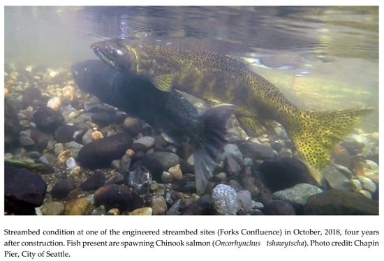
In support of this result, during autumn 2018, Chinook salmon were found spawning in the restored Forks Confluence [61]. This is the first documented spawning in this area ever since spawning surveys began in 1999, and is attributed to the improved streambed condition (which was visibly apparent in 2018, four years post-construction), the wider, more complex channel morphology, and restored hyporheic function providing the needed conditions to match spawning requirements.
6.8. Future Prospects of Hyporheic Restoration
Significant water quality benefits have been documented on a local scale by evaluating in detail a handful of parameters on an individual plunge-pool structure among the six plunge-pool structures in the Kingfisher restoration site and eight on the Confluence restoration site. Water quality within a stream is degraded by diffuse interactions with impervious surfaces, unshaded open water, and exposure to environmental chemicals occurring throughout the watershed. The next step is to explore how to correlate the amount of stream and hyporheic restoration, which is required to provide significant water quality benefits to treat that incoming pollution from a watershed, and how this work can be integrated into a larger vision which also incorporates current input-water engineered treatment solutions such as vegetated filter strips and stormwater retention structures. In the broadest sense, it is worth considering whether stream and hyporheic restoration, when implemented at scale throughout a watershed, serve as a superior replacement to current engineering practices and provide water quality enhancements with combined habitat uplift benefiting instream fauna as well as riparian functions including improvements to air quality, avian habitat, and soil moisture retention.
7. Conclusions
This new approach to enhanced hyporheic design successfully restored hyporheic processes and yielded significant water quality improvements compared to control and pre-project conditions. The engineered streambed and large-wood structures central to this design have yielded vertical water flux averaging 89 times greater than pre-project conditions, and with a maximum 16 times greater than that found in a pristine watercourse. Mapping of upwelling and downwelling zones in the restored reach yielded a surface-water to intra-gravel temperature difference 1.5 times that of the control reach and 4 times that of the pre-restoration reach, demonstrating the ability of the restoration design to yield an improved hyporheic circulation in summer conditions. Surface water longitudinal temperature patterns documented greater than 1.5 degrees of cooling as the water passed through a plunge-pool structure in full sun in the middle of the day, which can only be attributed to hyporheic exchange driving flows subsurface and subsequent cooling. Effective hyporheic zone cross section, as estimated by the immobile to mobile cross-section ratio, improved by a factor of 3.
The engineered streambed has been resilient to the influence of its sediment load. Surface and subsurface sand content, an indicator of hyporheic performance, has shown no observable tendency for the streambed to revert to the embedded, impermeable state that existed before project construction, at least over 2–3 years of sampling. The design has thus proven capable of maintaining natural scour and fill processes which slow or reverse embedded conditions and may actually improve over time through natural stream evolution, including processes of large-wood recruitment and associated accumulation of more diverse and extensive alluvial streambed material.
Other researchers studying the water chemistry and biology have shown that this hyporheic restoration has also been effective at significantly reducing concentrations of incoming pollutants [29], and at enhancing both hyporheic microbial heterotrophic production and macroinvertebrate taxa diversity and richness [37].
Supplementary Materials
The following are available online at https://www.mdpi.com/2073-4441/12/2/425/s1: Spreadsheet S1: Summary of computed vertical water flux, and Spreadsheet S2: Summary of surface-intragravel temperature differences.
Author Contributions
Conceptualization of engineered streambed design, P.D.B., M.H., and K.D.L.; formal project engineering design, M.H.; methodology, investigation, data curation, formal analysis, validation, visualization, and original draft preparation, P.D.B.; review and editing, P.D.B., K.D.L. and M.H.; resources, P.D.B. and K.D.L.; funding acquisition, K.D.L. All authors have read and agreed to the published version of the manuscript.
Funding
This research was funded by the City of Seattle, contract No. 14-133-A.
Acknowledgments
We thank Chapin Pier and Steve Damm (City of Seattle), Tracy Leavy, Kennith King, Alex Bell, Zach Moore, Michael Carlson and Michael Elam (U.S. Fish and Wildlife Service), Lila Neal and Corrine Hoffman (volunteers), Michaela Lowe, Jawad Frangieh and Jeffrey Lee (Americorps) for their diligent field assistance. We thank Jeffery Johnson (U.S. Fish and Wildlife Service), Michaela Lowe, Laurel Low, and Jeffery Lee (Americorps) for generous assistance with lab analysis of sediment. We thank Jeffrey Godden for software coding assistance. We also thank Jennifer Hrachovec for her thoughtful edits, Colin Riordan (Natural Systems Design) for help with map graphics and Danielle Devier (Natural Systems Design) for illustrations. We thank the U.S. Fish and Wildlife Service, under whose employment Paul D. Bakke (author) performed all of his work except for manuscript preparation. Finally, we give special thanks to Katherine D. Lynch, for her tenacious advocacy of this project to the City of Seattle leadership over many years, without which none of this would have been possible.
Conflicts of Interest
The authors declare no conflict of interest. Opinions expressed in this article represent those of the authors and not of the U.S. Fish and Wildlife Service, the City of Seattle, The Science of Rivers, or Natural Systems Design.
Appendix A

Table A1.
Streambed surface layer grain size statistics for all 9 Thornton Creek sites (see Figure A1).
Table A1.
Streambed surface layer grain size statistics for all 9 Thornton Creek sites (see Figure A1).
| Site | Year | Surface Grain Size Distribution (mm): | ||||
|---|---|---|---|---|---|---|
| D15 | D35 | D50 | D84 | D95 | ||
| Kingfisher Control, KFC | 2007 | 17.0 | 31.4 | 42.3 | 81.2 | 109.7 |
| 2015 | 15.5 | 39.4 | 58.2 | 87.0 | 111.4 | |
| 2017 | 6.7 | 24.3 | 45.7 | 96.7 | 117.3 | |
| Kingfisher Treatment, KFT1 | 2007 | 4.1 | 14.0 | 23.0 | 52.3 | 69.4 |
| 2015 | 20.2 | 30.0 | 35.5 | 51.1 | 59.7 | |
| 2017 | 14.6 | 26.5 | 32.2 | 51.4 | 61.3 | |
| Kingfisher Treatment, KFT2 | 2015 | 11.2 | 27.3 | 35.5 | 52.8 | 60.2 |
| 2017 | 0.6 | 18.9 | 28.9 | 50.4 | 65.7 | |
| South Fork Control, SFC | 2007 | 7.5 | 24.0 | 39.3 | 98.2 | 117.8 |
| 2016 | 8.5 | 25.4 | 36.6 | 68.7 | 82.7 | |
| 2017 | 7.3 | 21.8 | 34.2 | 68.1 | 82.5 | |
| South Fork Treatment, SFT1 | 2016 | 12.4 | 22.6 | 29.6 | 76.5 | 111.2 |
| 2017 | 13.4 | 23.4 | 28.4 | 54.3 | 76.0 | |
| South Fork Treatment, SFT2 | 2007 | 5.7 | 11.1 | 15.7 | 37.4 | 96.6 |
| 2016 | 2.5 | 10.3 | 17.8 | 39.5 | 59.7 | |
| 2017 | 3.2 | 10.7 | 16.9 | 29.9 | 39.9 | |
| North Fork Control, NFC | 2007 | 9.7 | 25.9 | 44.4 | 112.7 | 151.7 |
| 2016 | 4.5 | 15.3 | 23.2 | 46.5 | 57.9 | |
| 2017 | 7.4 | 25.3 | 34.0 | 53.0 | 61.5 | |
| North Fork Treatment, NFT | 2007 | 4.1 | 17.5 | 29.9 | 63.7 | 94.1 |
| 2016 | 9.0 | 20.8 | 28.6 | 90.7 | 114.9 | |
| 2017 | 7.9 | 17.6 | 23.2 | 34.0 | 42.3 | |
| Mainstem Treatment, MST | 2016 | 2.9 | 22.1 | 26.3 | 44.0 | 59.0 |
| 2017 | 11.0 | 24.5 | 30.1 | 55.7 | 69.9 | |
Table A2.
Streambed subsurface layer grain size statistics for all 9 Thornton Creek sites (see Figure A1).
Table A2.
Streambed subsurface layer grain size statistics for all 9 Thornton Creek sites (see Figure A1).
| Site | Year | Subsurface Grain Size Distribution (mm) | ||||
|---|---|---|---|---|---|---|
| D15 | D35 | D50 | D84 | D95 | ||
| Kingfisher Control, KFC | 2007 | 3.0 | 10.2 | 18.4 | 51.1 | 67.3 |
| 2015 | 2.8 | 13.1 | 27.0 | 81.4 | 110.8 | |
| 2017 | 1.1 | 7.1 | 15.4 | 62.6 | 88.7 | |
| Kingfisher Treatment, KFT1 | 2007 | 2.5 | 9.2 | 17.7 | 53.6 | 75.4 |
| 2015 | 2.9 | 13.7 | 23.5 | 36.6 | 47.0 | |
| 2017 | 6.1 | 24.5 | 30.0 | 50.4 | 61.2 | |
| Kingfisher Treatment, KFT2 | 2015 | 4.4 | 8.7 | 17.2 | 33.7 | 49.0 |
| 2017 | 2.6 | 7.9 | 14.8 | 35.4 | 43.4 | |
| South Fork Control, SFC | 2007 | 2.6 | 8.8 | 16.3 | 42.8 | 62.0 |
| 2016 | 1.0 | 6.2 | 12.9 | 45.9 | 62.5 | |
| 2017 | 1.5 | 7.0 | 14.3 | 53.6 | 77.7 | |
| South Fork Treatment, SFT1 | 2016 | 3.1 | 15.3 | 24.2 | 47.7 | 60.2 |
| 2017 | 2.7 | 12.6 | 20.3 | 36.5 | 44.9 | |
| South Fork Treatment, SFT2 | 2007 | 1.8 | 7.4 | 12.7 | 30.4 | 41.6 |
| 2016 | 1.9 | 14.3 | 25.0 | 52.4 | 74.5 | |
| 2017 | 0.6 | 3.3 | 6.8 | 23.1 | 30.2 | |
| North Fork Control, NFC | 2007 | 3.3 | 10.3 | 18.1 | 48.5 | 68.7 |
| 2016 | 1.0 | 7.0 | 14.7 | 38.9 | 56.4 | |
| 2017 | 1.9 | 20.3 | 31.0 | 55.6 | 75.5 | |
| North Fork Treatment, NFT | 2007 | 1.7 | 7.7 | 14.5 | 38.6 | 54.6 |
| 2016 | 2.5 | 12.9 | 22.7 | 44.6 | 60.0 | |
| 2017 | 1.5 | 10.3 | 18.2 | 46.4 | 77.8 | |
| Mainstem Treatment, MST | 2016 | 1.0 | 16.6 | 23.7 | 40.2 | 103.5 |
| 2017 | 11.0 | 24.5 | 30.1 | 55.7 | 69.9 | |

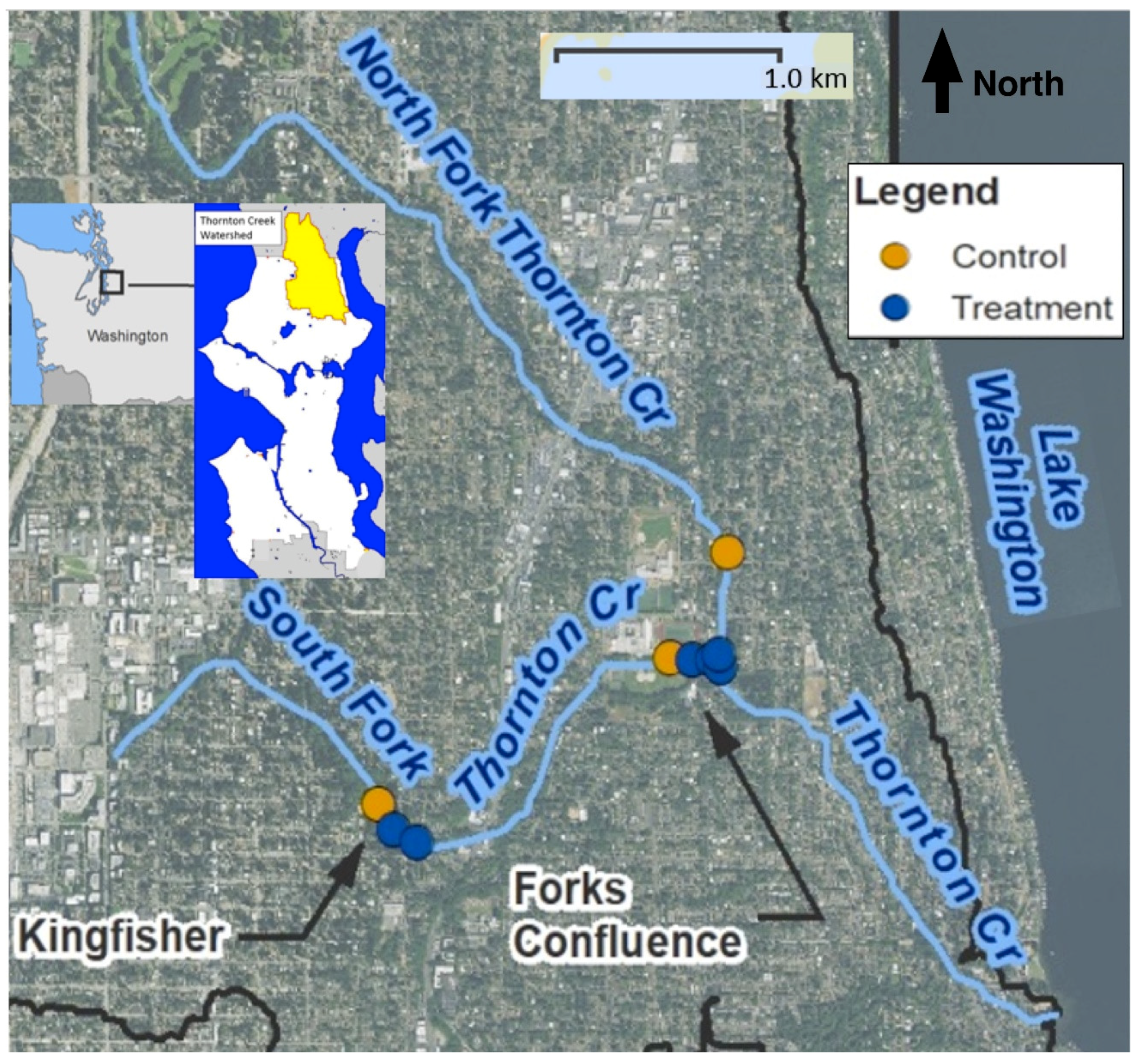
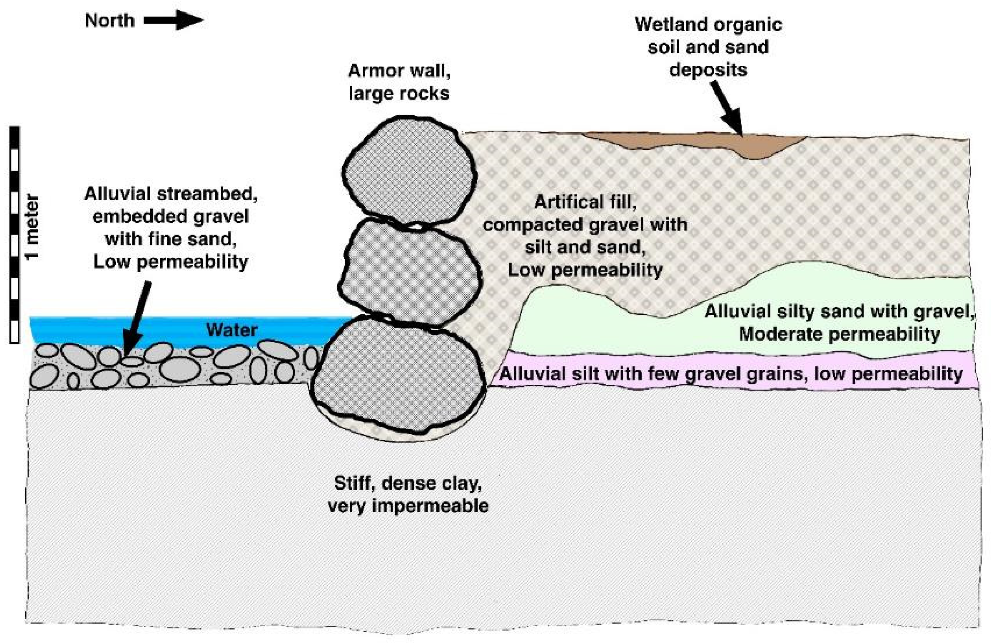
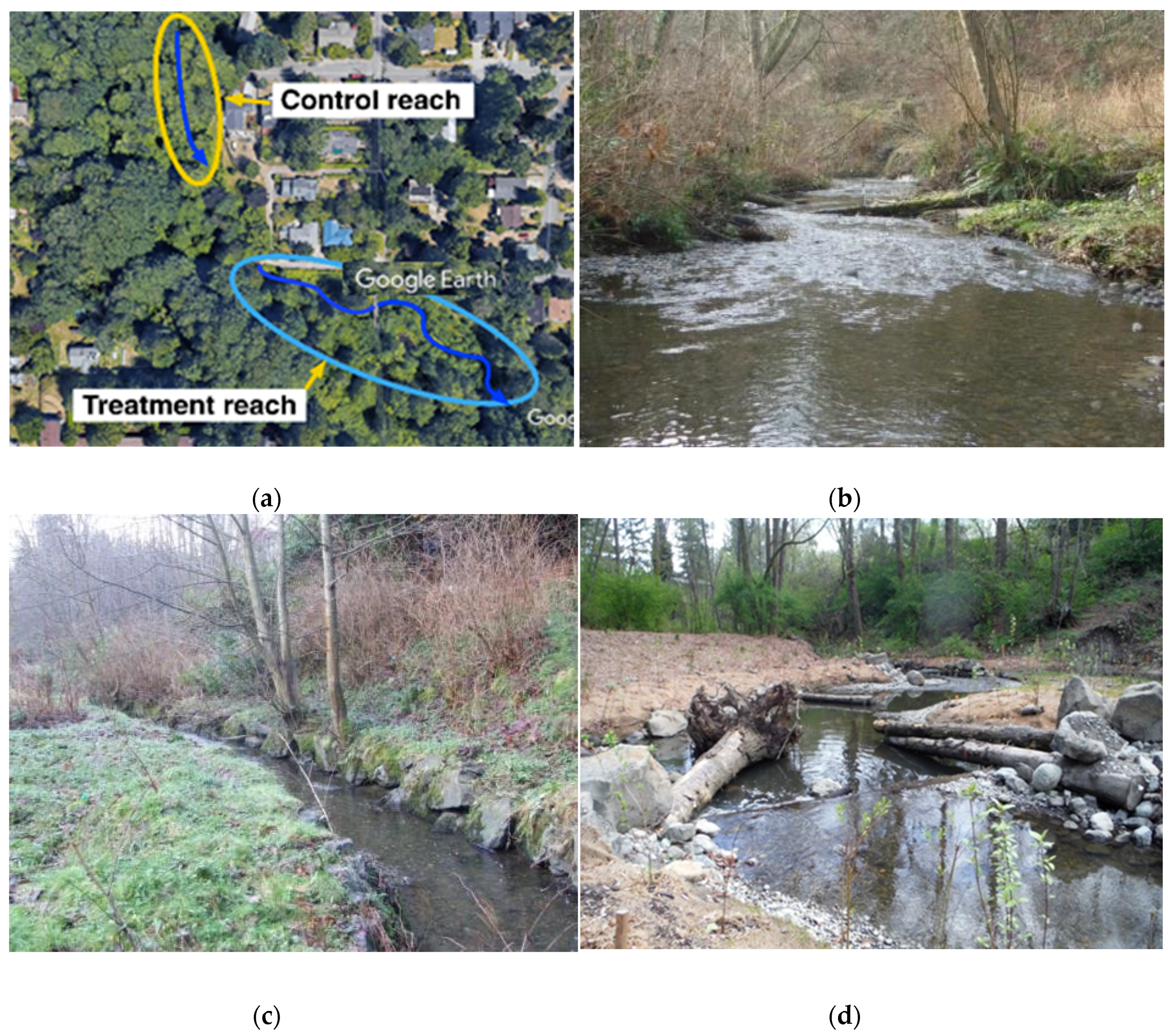
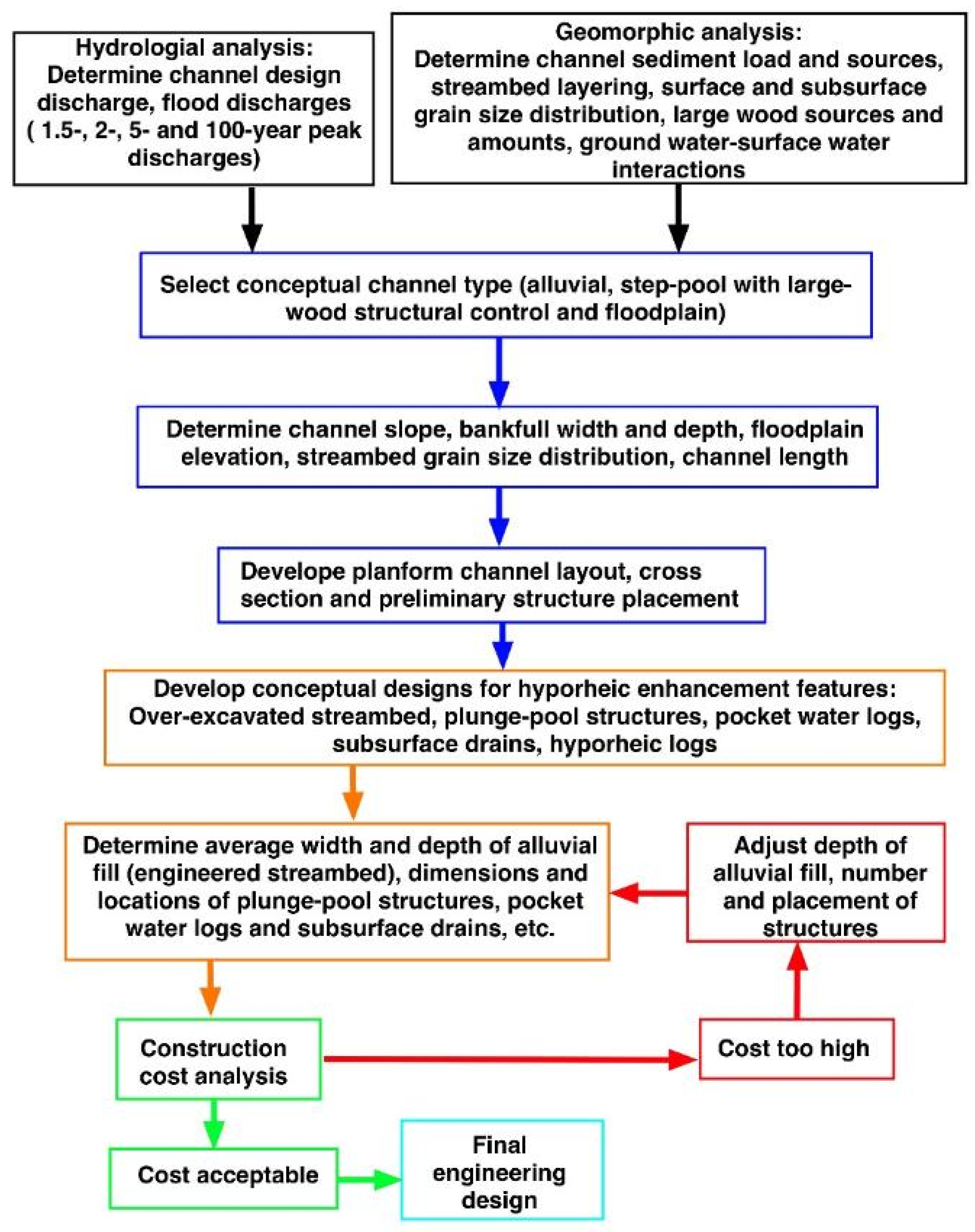
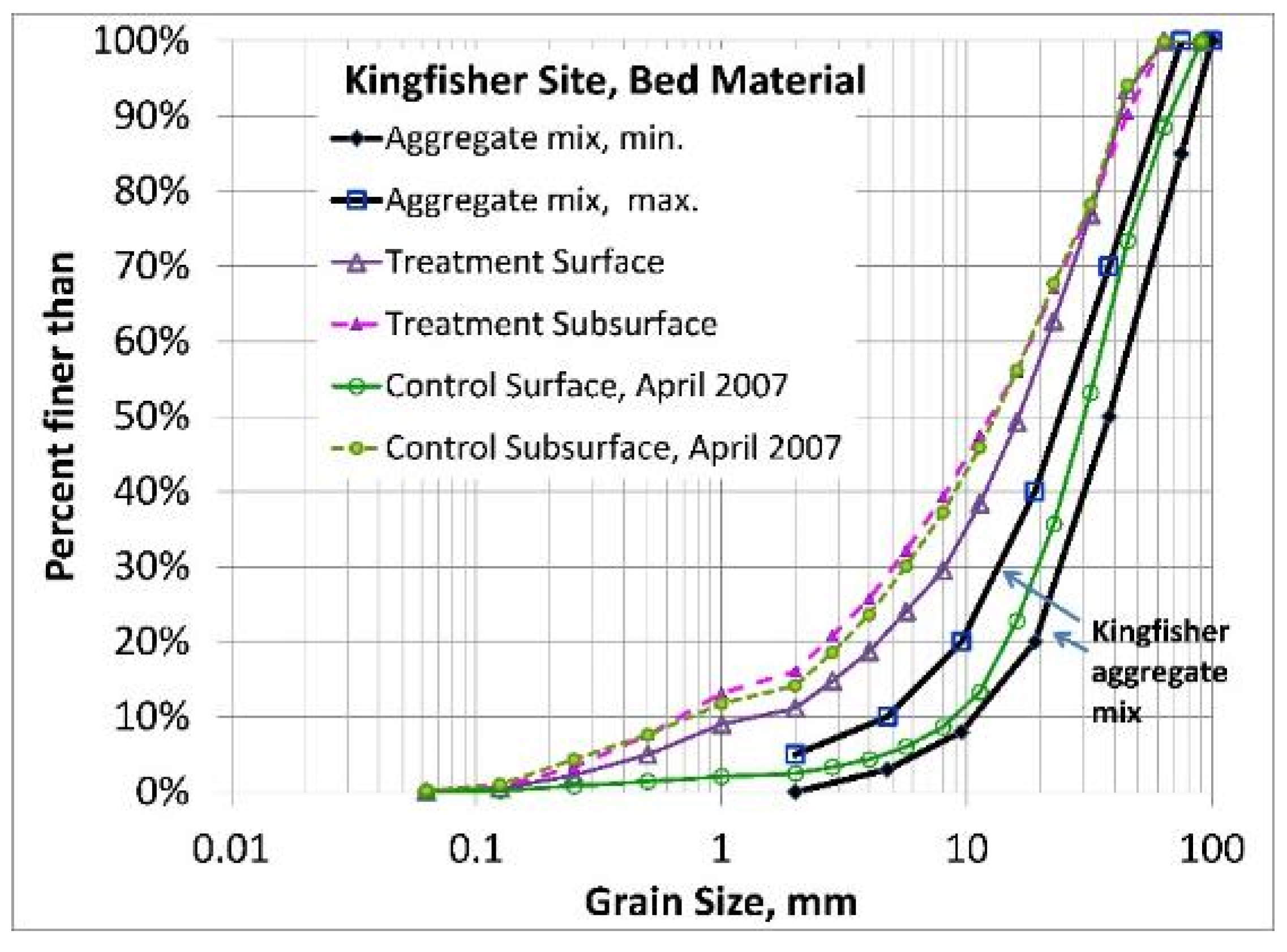
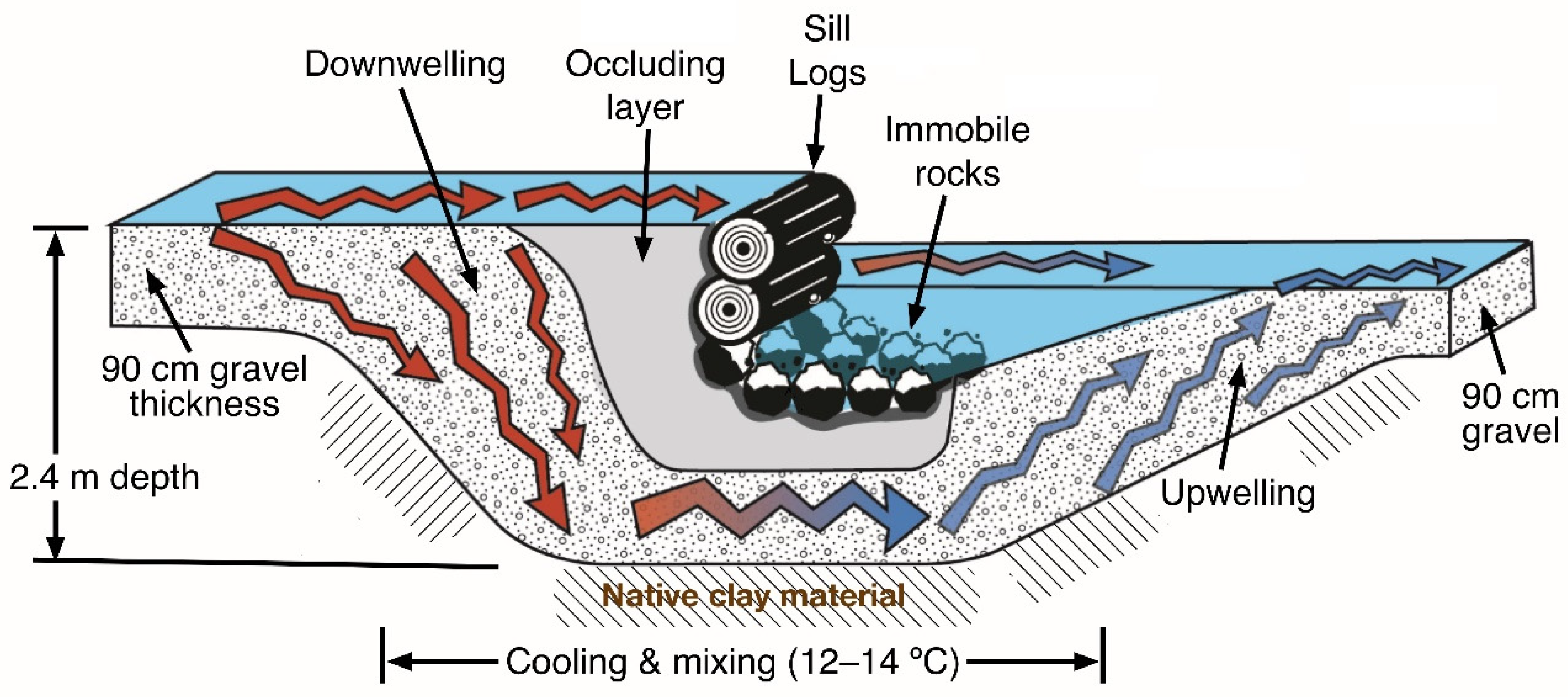
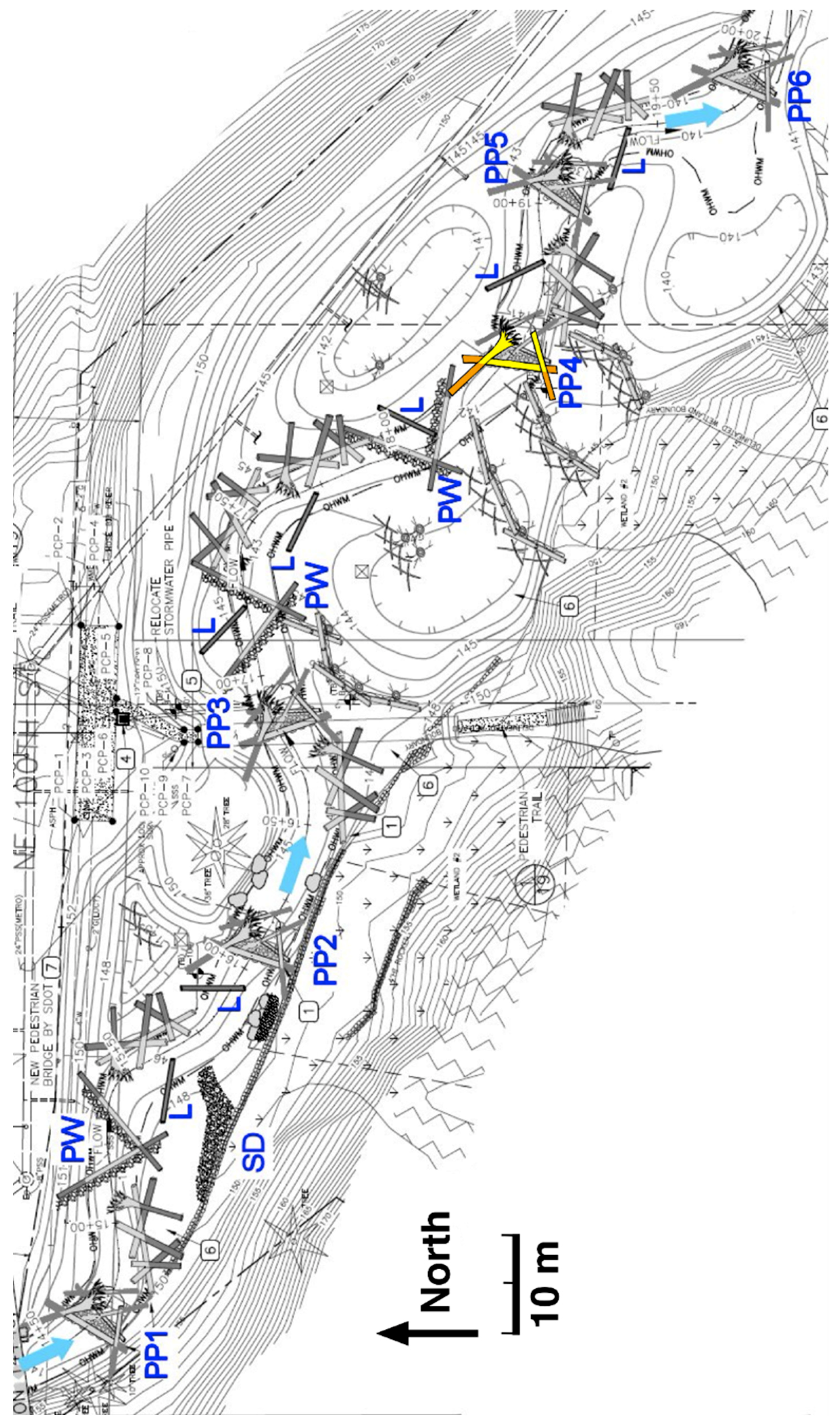
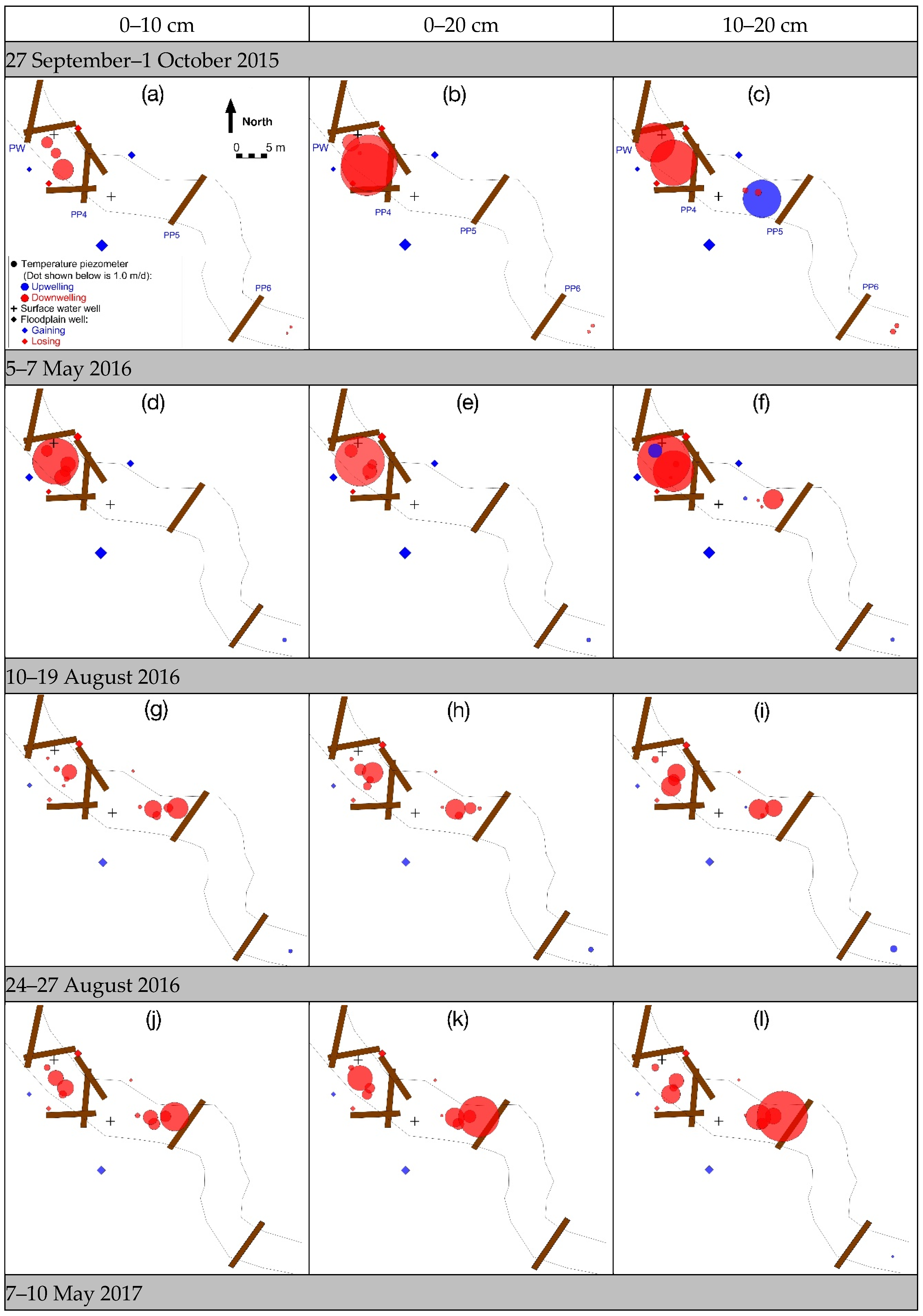
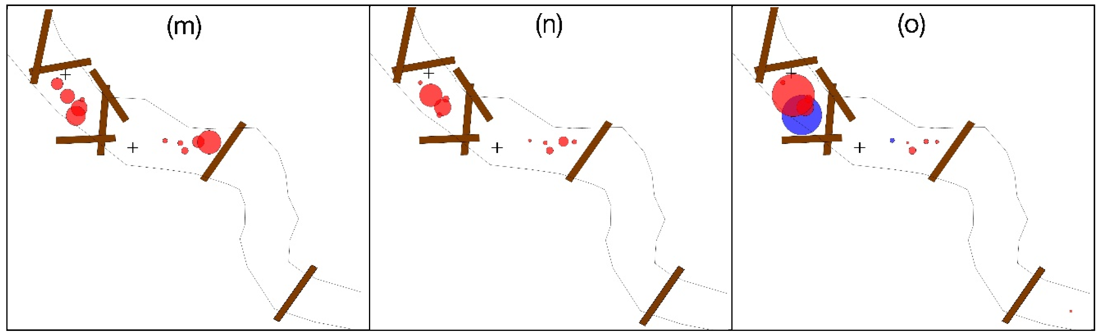
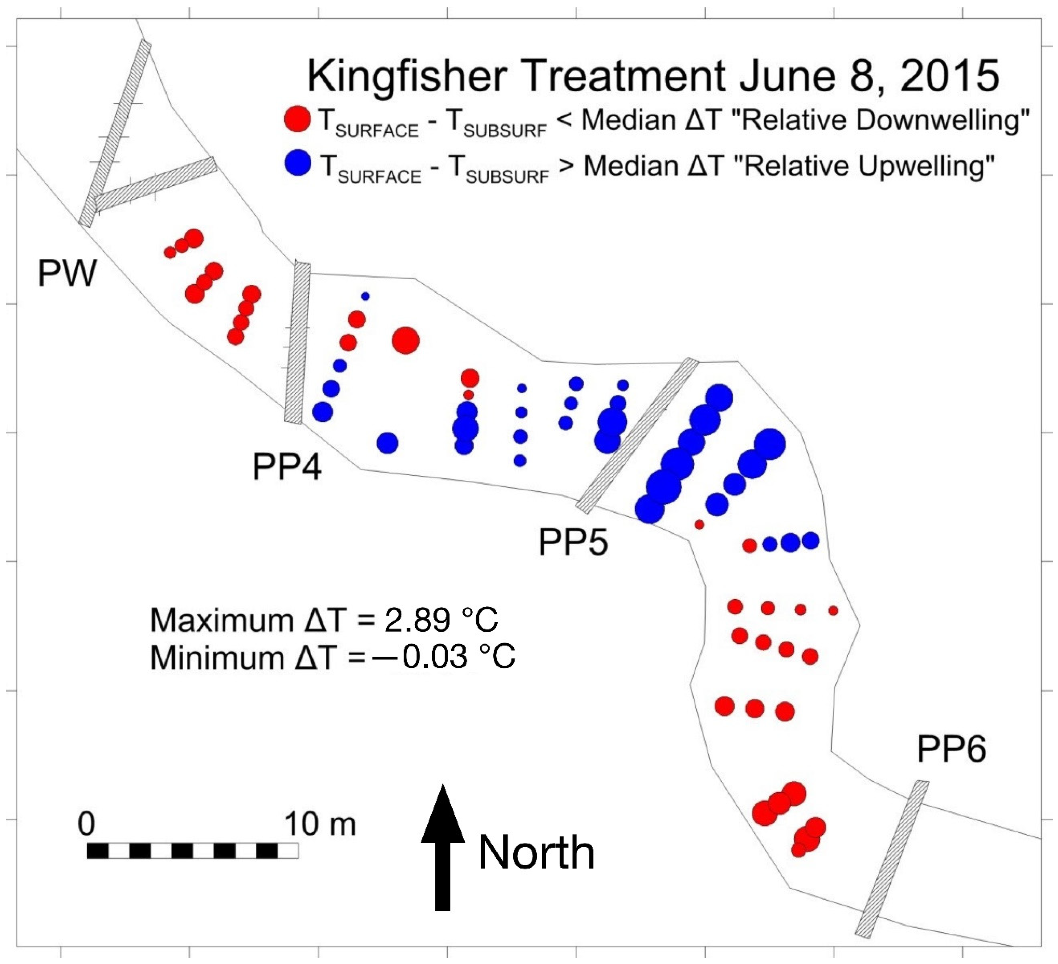
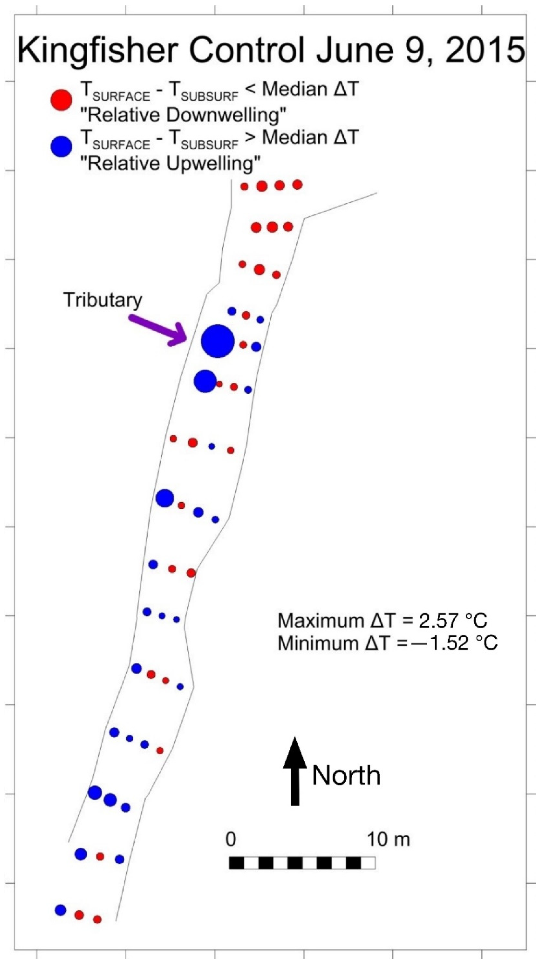
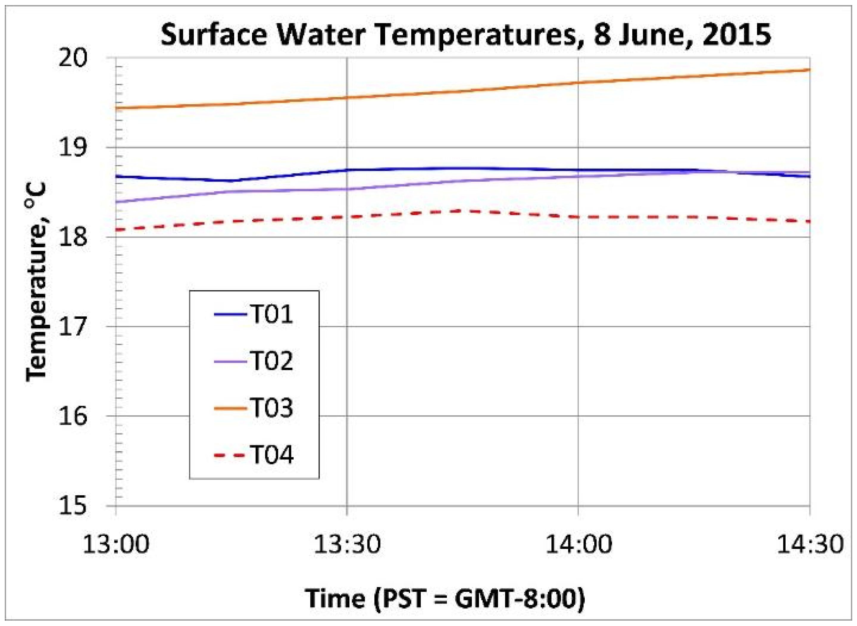
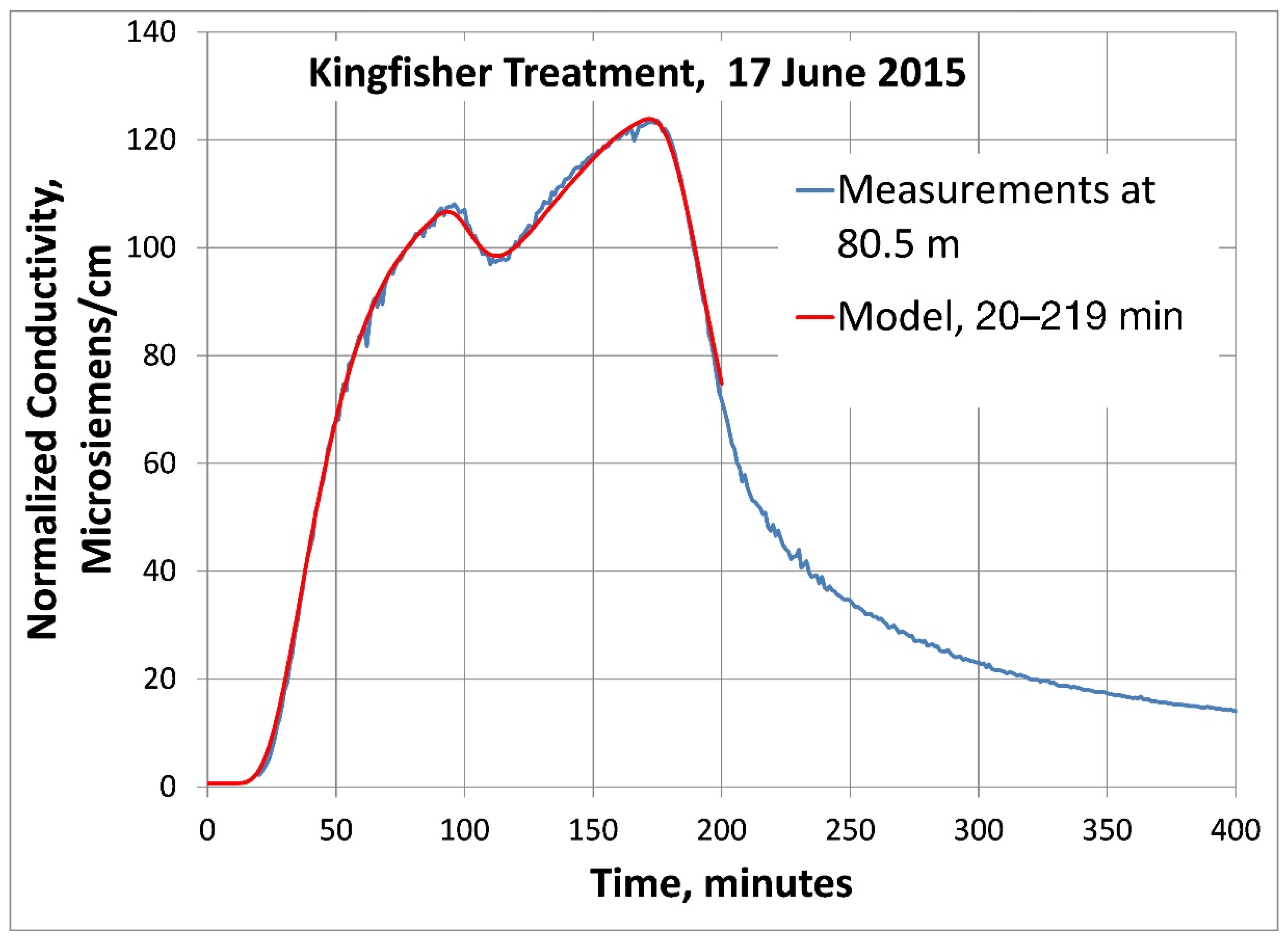
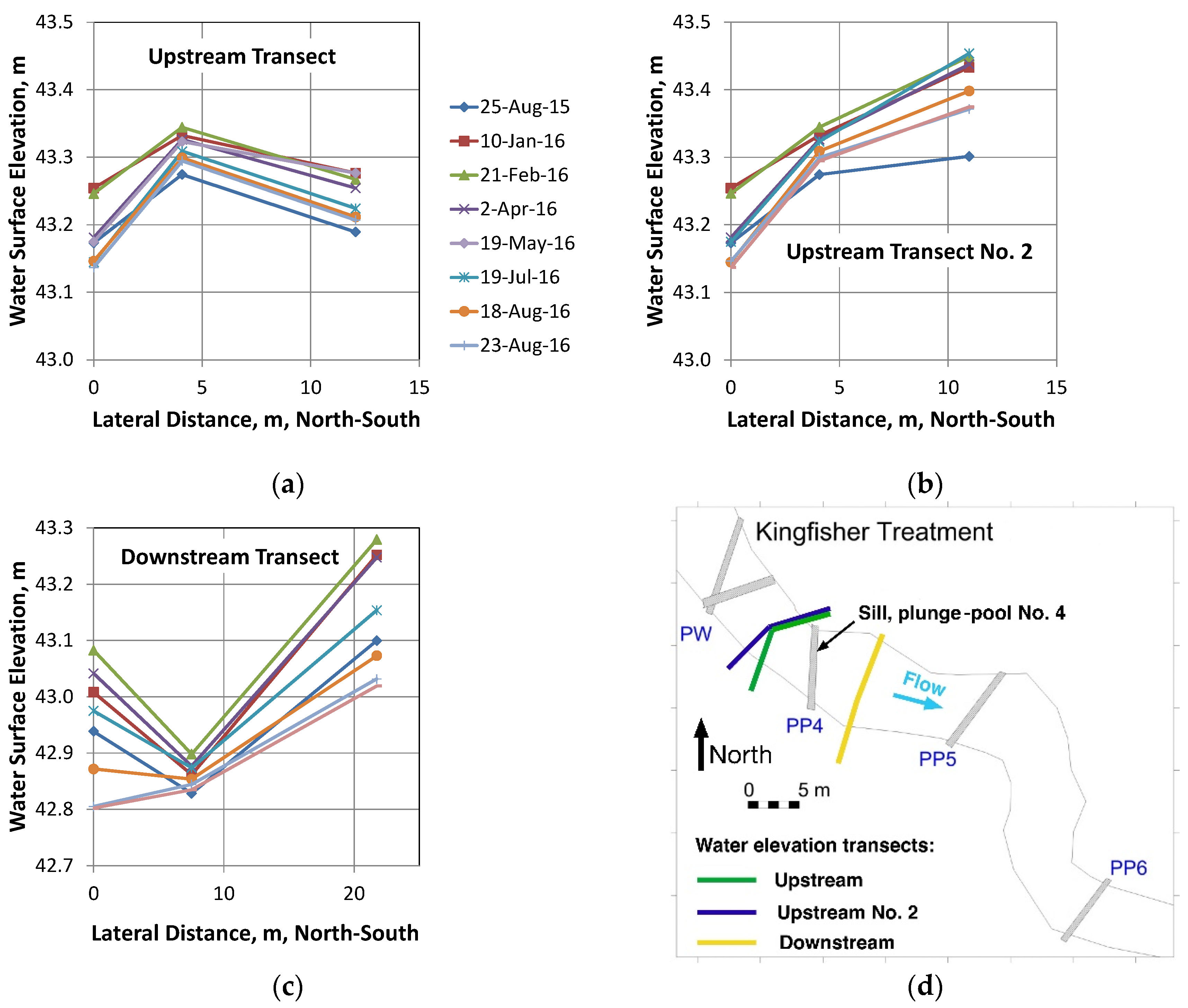
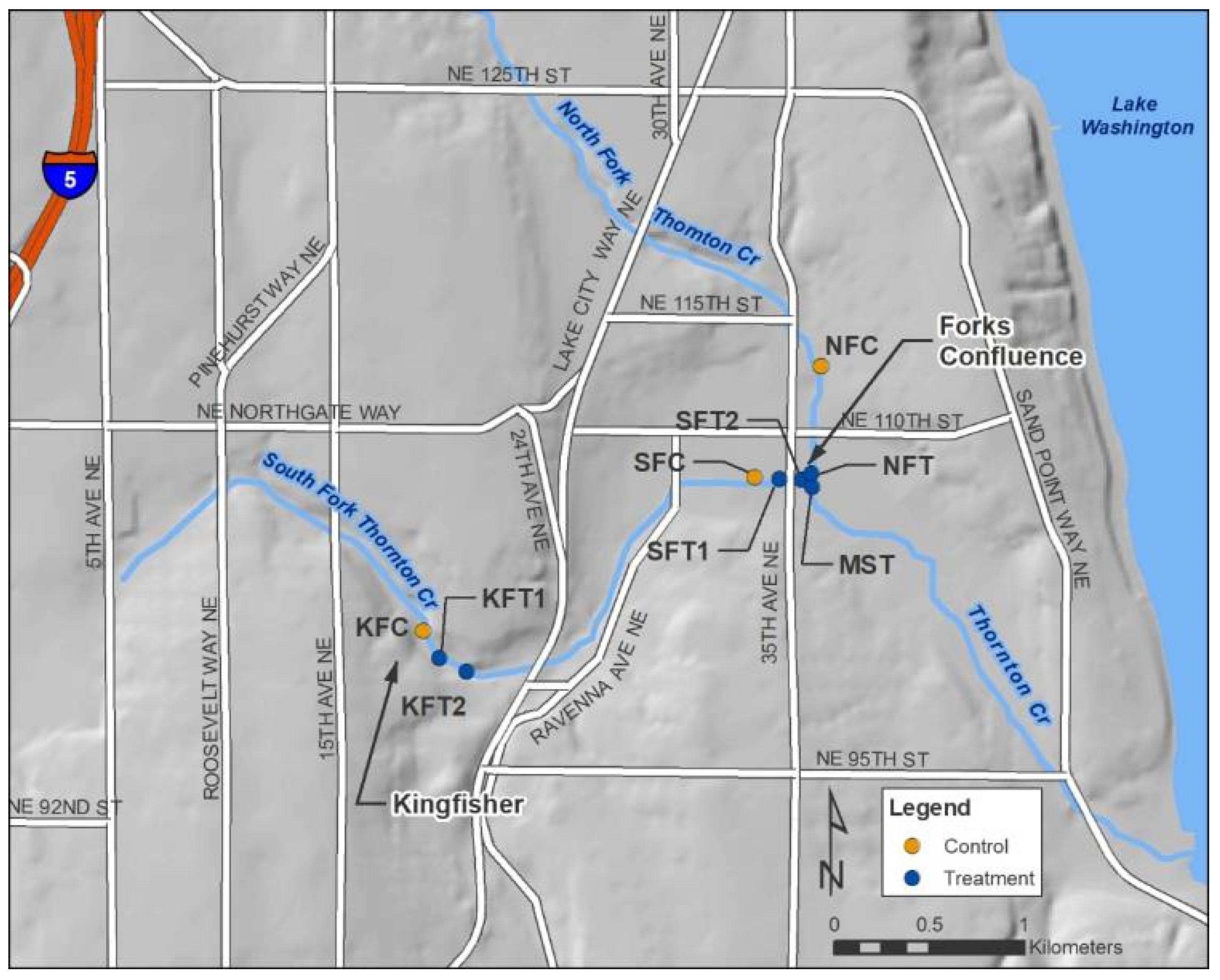
References
- Federal Interagency Stream Restoration Working Group (FISRWG). Stream Corridor Restoration: Principles, Processes, and Practices; U.S. Government: Washington, DC, USA, 1998; ISBN -0-934213-59-3.
- Budd, W.W.; Cohen, P.L.; Saunders, P.R.; Steiner, F.R. Stream corridor management in the Pacific Northwest: I. Determination of stream-corridor widths. Environ. Mgmnt. 1987, 11, 587–597. [Google Scholar] [CrossRef]
- Stanford, J.A.; Ward, J.V. An ecosystem perspective of alluvial rivers: Connectivity and the hyporheic corridor. Jour. N. Am. Benth. Soc. 1993, 12, 48–60. [Google Scholar] [CrossRef]
- Buss, S.; Cai, Z.; Cardenas, B.; Fleckenstein, J.; Hannah, D.; Heppell, K.; Wood, P. The Hyporheic Handbook: A Handbook on the Groundwater-Surface Water Interface and Hyporheic Zone for Environment Managers; Integrated Catchment Science Programme: Bristol, UK, 2009; ISBN 9781849111317. [Google Scholar]
- Edwards, R.T. The Hyporheic Zone. In River Ecology and Management: Lessons from the Pacific Coastal Ecosystem; Naiman, R.J., Bilby, R.E., Eds.; Springer: New York, NY, USA, 1998; pp. 399–429. ISBN 978-0-387-95246-8. [Google Scholar]
- Cardenas, M.B. Hyporheic zone hydrological science: A historical account of its emergence and a prospectus. Water Resour. Res. 2015, 51, 3601–3616. [Google Scholar] [CrossRef]
- Harvey, J.; Gooseff, M. River corridor science: Hydrologic exchange and ecological consequences from bedforms to basins. Water Resour. Res. 2015, 51, 6893–6922. [Google Scholar] [CrossRef] [Green Version]
- Fischer, H.; Kloep, F.; Wilzcek, S.; Pusch, M.T. A river’s liver: Microbial processes within the hyporheic zone of a large lowland river. Biogeochemistry 2005, 76, 349–371. [Google Scholar] [CrossRef]
- Stanford, J.A.; Ward, J.V. The hyporheic habitat of river of river ecosystems. Nature 1988, 335, 64–66. [Google Scholar] [CrossRef]
- Hester, E.T.; Doyle, M.W. In-stream geomorphic structures as drivers of hyporheic exchange. Water Resour. Res. 2008, 44. [Google Scholar] [CrossRef]
- Ward, A.S.; Gooseff, M.N.; Johnson, P.A. How can subsurface modifications to hydraulic conductivity be designed as stream restoration structures? Analysis of Vaux’s conceptual models to enhance hyporheic exchange. Water Resour. Res. 2011, 47. [Google Scholar] [CrossRef]
- Boulton, A.J. Hyporheic rehabilitation in rivers: Restoring vertical connectivity. Freshwater Biol. 2007, 52, 632–650. [Google Scholar] [CrossRef]
- Barnard, R.J.; Johnson, J.; Brooks, P.; Bates, K.M.; Heiner, B.; Klavas, J.P.; Ponder, D.C.; Smith, P.D.; Powers, P.D. Water Crossings Design Guidelines; Washington Department of Fish and Wildlife: Olympia, WA, USA, 2013; pp. 28–69. Available online: https://wdfw.wa.gov/publications/01501 (accessed on 29 January 2020).
- Herzog, S.P.; Higgins, C.P.; McCray, J.E. Engineered streambeds for induced hyporheic flow: Enhanced removal of nutrients, pathogens, and metals from urban streams. J. Environ. Eng. 2015, 142, 04015053-1–04015053-10. [Google Scholar] [CrossRef]
- Crispell, J.K.; Endreny, T.A. Hyporheic exchange flow around constructed in-channel structures and implications for restoration design. Hydrol. Process. 2009, 23, 1158–1168. [Google Scholar] [CrossRef]
- Washington State Dept. of Transportation (WSDOT). Stormwater best management practices. In Highway Runoff Manual, M31-16.04, Suppl. February 2016; Washington State Dept. of Transportation: Olympia, WA, USA, 2016; pp. 5-1–5-227. Available online: https://www.wsdot.wa.gov/Publications/Manuals/M31-16.htm (accessed on 29 January 2020).
- McIntyre, J.K.; Davis, J.W.; Hinman, C.; Macneale, K.H.; Anulacion, B.F.; Scholz, N.L.; Stark, J.D. Soil bioretention protects juvenile salmon and their prey from the toxic impacts of urban stormwater runoff. Chemosphere 2015, 132, 213–219. [Google Scholar] [CrossRef] [PubMed] [Green Version]
- Spromberg, J.A.; Baldwin, D.H.; Damm, S.E.; McIntyre, J.K.; Huff, M.; Sloan, C.A.; Anulacion, B.F.; Davis, J.W.; Scholz, N.L. Coho salmon spawner mortality in western US urban watersheds: Bioinfiltration prevents lethal storm water impacts. J. Appl. Ecol. 2016, 53, 398–407. [Google Scholar] [CrossRef] [PubMed]
- Böhlke, J.K.; Antweiler, R.C.; Harvey, J.W.; Laursen, A.E.; Smith, L.K.; Smith, R.L.; Voytek, M.A. Multi-scale measurements and modeling of denitrification in streams with varying flow and nitrate concentration in the upper Mississippi river basin, USA. Biogeochemical 2009, 93, 117–141. [Google Scholar] [CrossRef] [Green Version]
- Böhlke, J.K.; Harvey, J.W.; Voytek, M.A. Reach-scale isotope tracer experiment to quantify denitrification and related processes in a nitrate-rich stream, midcontinent United States. Limnol. Oceanogr. 2004, 49, 821–838. [Google Scholar] [CrossRef]
- Butturini, A.; Sabater, F. Importance of transient storage zones for ammonium and phosphate retention in a sandy-bottom Mediterranean stream. Freshwater Biol. 1999, 41, 593–603. [Google Scholar] [CrossRef]
- Groffman, P.M.; Altabet, M.A.; Böhlke, J.K.; Butterbach-Bahl, K.; David, M.B.; Firestone, M.K.; Giblin, A.E.; Kana, T.M.; Nielsen, L.P.; Voytek, M.A. Methods for measuring denitrification: Diverse approaches to a difficult problem. Ecol. Appl. 2006, 16, 2091–2122. [Google Scholar] [CrossRef]
- Lewandowski, J.; Putschew, A.; Schwesig, D.; Neumann, C.; Radke, M. Fate of organic micropollutants in the hyporheic zone of a eutrophic lowland stream: Results of a preliminary field study. Sci. Total Environ. 2011, 409, 1824–1835. [Google Scholar] [CrossRef]
- Mulholland, P.J.; Valett, H.M.; Webster, J.R.; Thomas, S.A.; Cooper, L.W.; Hamilton, S.K.; Peterson, B.J. Stream denitrification and total nitrate uptake rates measured using a field 15N tracer addition approach. Limnol. Oceanogr. 2004, 49, 809–820. [Google Scholar] [CrossRef]
- Mulholland, P.J.; Helton, A.M.; Poole, G.C.; Hall, R.O.; Hamilton, S.K.; Peterson, B.J.; Tank, J.L.; Ashkenas, L.R.; Cooper, L.W.; Dahm, C.N.; et al. Stream denitrification across biomes and its response to anthropogenic nitrate loading. Nature 2008, 452, 202–205. [Google Scholar] [CrossRef]
- Orr, C.H.; Predick, K.I.; Stanley, E.H.; Rogers, K.L. Spatial autocorrelation of denitrification in a restored and a natural floodplain. Wetlands 2014, 34, 89–100. [Google Scholar] [CrossRef]
- Poole, G.C.; Berman, C.H. An ecological perspective on in-stream temperature: Natural heat dynamics and mechanisms of human-caused thermal degradation. Environ. Mgmnt. 2000, 27, 787–802. [Google Scholar] [CrossRef] [PubMed]
- Burkholder, B.K.; Grant, G.E.; Haggerty, R.; Khangaonkar, T.; Wampler, P.J. Influence of hyporheic flow and geomorphology on temperature of a large, gravel-bed river, Clackamas River, Oregon, USA. Hydrol. Process. 2008, 22, 941–953. [Google Scholar] [CrossRef]
- Peter, K.T.; Tian, Z.; Wu, C.; Lin, P.; White, S.; Du, B.; McIntyre, J.K.; Scholz, N.L.; Kolodziej, E.P. Using high-resolution mass spectrometry to identify organic contaminants linked to urban stormwater mortality syndrome in Coho Salmon. Environ. Sci. Technol. 2018. [Google Scholar] [CrossRef]
- Peter, K.T.; Herzog, S.; Tian, Z.; McCray, J.; Lynch, K.; Kolodziej, E.P. Evaluating emerging organic contaminant removal in an engineered hyporheic zone using high resolution mass spectrometry. Water Res. 2019, 150, 140–152. [Google Scholar] [CrossRef]
- Spromberg, J.A.; Scholz, N.L. Estimating the future decline of wild Coho salmon populations resulting from early spawner die-offs in urbanizing watersheds of the Pacific Northwest, USA. Integr. Environ. Assess. Manag. 2011, 7, 648–656. [Google Scholar] [CrossRef] [Green Version]
- Feist, B.E.; Buhle, E.R.; Arnold, P.; Davis, J.W.; Scholz, N.L. Landscape ecotoxicology of Coho salmon spawner mortality in urban streams. PLoS ONE 2011, 6, e23424. [Google Scholar] [CrossRef]
- Feist, B.E.; Buhle, E.R.; Baldwin, D.H.; Spromberg, J.A.; Damm, S.E.; Davis, J.W.; Scholz, N.L. Roads to ruin: Conservation threats to a sentinel species across an urban gradient. Ecol. Appl. 2017, 27, 2382–2396. [Google Scholar] [CrossRef] [Green Version]
- Scholz, N.L.; Myers, M.S.; McCarthy, S.G.; Labenia, J.S.; McIntyre, J.K.; Ylitalo, G.M.; Rhodes, L.D.; Laetz, C.A.; Stehr, C.M.; French, B.L.; et al. Recurrent die-offs of adult Coho salmon returning to spawn in Puget Sound lowland urban streams. PLoS ONE 2011, 6, e28013. [Google Scholar] [CrossRef]
- Harris, G.P.; Heathwaite, A.L. Why is achieving good ecological outcomes in rivers so difficult? Freshwater Biol. 2011, 57, 91–107. [Google Scholar] [CrossRef]
- Lawrence, J.E.; Skold, M.E.; Hussain, F.; Silverman, D.R.; Resh, V.H.; Sedlak, D.L.; Luthy, R.; Mccray, J.E. Hyporheic zone in urban streams: A review and opportunities for enhancing water quality and improving aquatic habitat by active management. Environ. Engr. Sci. 2013, 30, 480–501. [Google Scholar] [CrossRef]
- Morley, S.; Rhodes, L.; Baxter, A.; Goetz, G. Biological outcomes of hyporheic zone restoration in an urban floodplain. In Proceedings of the 2018 Annual Stream Restoration Symposium, Stevenson, WA, USA, 5–8 February 2018; River Restoration Northwest: Portland, OR, USA, 2018. Available online: http://www.rrnw.org/wp-content/uploads/1.4_2018-02-River-Restoration-NW-Talk-Morley.pdf (accessed on 7 December 2018).
- Hall, J.; Basketfield, S.; Cooksey, M.; Zisette, R. City of Seattle State of the Waters 2007, Vol. 1: Seattle Water Courses; City of Seattle: Seattle, WA, USA, 2007; pp. 150–187. Available online: https://www.seattle.gov/util/cs/groups/public/@spu/@conservation/documents/webcontent/spu01_003413.pdf (accessed on 7 December 2018).
- Leavy, T.R.; Bakke, P.; Peters, R.J.; Morley, S. Influence of Habitat Complexity and Floodplain Reconnection Projects on the Physical and Biological Conditions of Seattle Urban Streams: Pre-Project Monitoring; Final Draft Report, 2005–2009; U.S. Fish and Wildlife Service: Lacey, WA, USA, 2010.
- Walsh, C.J.; Roy, A.H.; Feminella, J.W.; Cottingham, P.D.; Groffman, P.M.; Morgan, R.P. The urban stream syndrome: Current knowledge and the search for a cure. J. N. Am. Benthol. Soc. 2005, 24, 706–723. [Google Scholar] [CrossRef]
- Bakke, P.D. Thornton Creek Floodplain Restoration: Effectiveness Monitoring of Physical Processes; Report to City of Seattle, Vol. 1, Contract 14-133-A; U.S. Fish and Wildlife Service: Lacey, DC, USA, 2018; pp. 1–56.
- Bakke, P.D.; Lynch, K.; Leavy, T.; Peters, R. Monitoring of groundwater-surface water interactions in support of restoration of hyporheic processes in an urban stream, Thornton Creek, Washington (poster). In Proceedings of the Geological Society of America Annual Meeting, Portland, OR, USA, 20 October 2009. [Google Scholar]
- Washington Dept. of Fish and Wildlife (WDFW); U.S. Fish and Wildlife Service (USFWS). Technique 6, Instream structures. In Stream Habitat Restoration Guidelines; Cramer, M.L., Ed.; Co-published by the Washington Departments of Fish and Wildlife, Natural Resources, Transportation and Ecology, Washington State Recreation and Conservation Office, Puget Sound Partnership, and the U.S. Fish and Wildlife Service: Olympia, DC, USA, 2012; pp. T6-1–T6-36. [Google Scholar]
- Baxter, C.V.; Hauer, F.R. Geomorphology, hyporheic exchange, and selection of spawning habitat by bull trout. Can. J. Fish. Aquat. Sci. 2000, 57, 1470–1481. [Google Scholar] [CrossRef]
- Bjornn, T.C.; Reiser, D.W. Habitat requirements of salmonids in streams. In Influences of Forest and Rangeland Management on Salmonids Fishes and Their Habitats, American Fisheries Society Special Publication 19; Meehan, W.R., Ed.; American Fisheries Society: Bethesda, MD, USA, 1991; pp. 83–138. [Google Scholar]
- Gariglio, F.P.; Tonina, D.; Luce, C.H. Spatiotemporal variability of hyporheic exchange through a pool-riffle sequence. Water Resour. Res. 2009, 49, 1–20. [Google Scholar] [CrossRef]
- Luce, C.H.; Tonina, D.; Gariglio, F.; Applebee, R. Solutions for the diurnally forced advection-diffusion equation to estimate bulk fluid velocity and diffusivity in streambeds from temperature time series. Water Resour. Res. 2013, 49, 488–506. [Google Scholar] [CrossRef] [Green Version]
- Conant Jr., B. Delineating and quantifying ground water discharge zones using streambed temperatures. Groundwater 2004, 42, 243–257. [Google Scholar] [CrossRef]
- Webster, J.R.; Ehrman, T.P. Solute dynamics. In Methods in Stream Ecology; Hauer, F.R., Lambert, G.A., Eds.; Academic Press: New York, NY, USA, 1996; pp. 145–160. ISBN 0-12-332905-1. [Google Scholar]
- Runkel, R.L. One-Dimensional Transport with Inflow and Storage (OTIS): A Solute Transport Model for Streams and Rivers; Water-Resour. Invest. Rept. 98–4018; U.S. Geological Survey: Denver, CO, USA, 1998. [CrossRef]
- Bencala, K.E.; Walters, R.A. Simulation of solute transport in a mountain pool-and-riffle stream–a transient storage model. Water Resour. Res. 1983, 19, 718–724. [Google Scholar] [CrossRef]
- McNamara, M.L.; Klingeman, P.C.; Bakke, P.D.; Sullivan, R.L. Channel maintenance flows in the upper Klamath Basin, Oregon. In Riparian Ecology and Management in Multi-Land Use Watersheds; Wigington, P.J., Beschta, R.L., Eds.; TPS-00-2; American Water Resources Association: Middleberg, VA, USA, 2000; pp. 53–58. ISBN 978-1882132515. [Google Scholar]
- Bunte, K.; Abt, S.R. Sampling Surface and Subsurface Particle-Size Distributions in Wadable Gravel-and Cobble-Bed Streams for Analyses in Sediment Transport, Hydraulics, and Streambed Monitoring; General Technical Report RMRS-GTR-74; U.S. Department of Agriculture, Forest Service, Rocky Mountain Research Station: Fort Collins, CO, USA, 2001. [CrossRef]
- Wagner, B.J.; Harvey, J.W. Experimental design for estimating parameters of rate-limited mass transfer: Analysis of stream tracer studies. Water Resour. Res. 1997, 33, 1731–1741. [Google Scholar] [CrossRef] [Green Version]
- Buffington, J.M.; Tonina, D. Hyporheic exchange in mountain rivers I: Mechanics and environmental effects. Geogr. Compass 2009, 3, 1063–1086. [Google Scholar] [CrossRef]
- Buffington, J.M.; Tonina, D. Hyporheic exchange in mountain rivers II: Effects of channel morphology on mechanics, scales, and rates of exchange. Geogr. Compass 2009, 3, 1038–1062. [Google Scholar] [CrossRef]
- Sambrook Smith, G.H.; Nicholas, A.P.; Ferguson, R.I. Measuring and defining bimodal sediments. Water Resour. Res. 1997, 33, 1179–1185. [Google Scholar] [CrossRef]
- Kondolf, G.M.; Li, S. The pebble count technique for quantifying surface bed material size in instream flow studies. Rivers 1992, 3, 80–87. [Google Scholar]
- Parker, G.; Toro-Escobar, C.M. Equal mobility of gravel in streams: The remains of the day. Water Resour. Res. 2002, 38, 1–8. [Google Scholar] [CrossRef]
- Hyatt, T.L.; Naiman, R.J. The residence time of large wood debris in the Queets River, Washington, USA. Ecol. Apps. 2001, 11, 191–202. [Google Scholar] [CrossRef]
- Lynch, K.; Seattle Public Utilities, Seattle, WA, USA; Pier, C.; Seattle Public Utilities, Seattle, WA, USA. Personal communication, 2018.
Figure 1.
Locations of control and treatment sites for both Seattle Public Utilities (SPU) Thornton Floodplain projects. Right inset shows the watershed (yellow) within the City of Seattle (white). Left inset is a portion of Washington State, USA. Scale shows 1 km = 0.6 mile.
Figure 1.
Locations of control and treatment sites for both Seattle Public Utilities (SPU) Thornton Floodplain projects. Right inset shows the watershed (yellow) within the City of Seattle (white). Left inset is a portion of Washington State, USA. Scale shows 1 km = 0.6 mile.

Figure 2.
Schematic pre-construction substrate cross section at the Kingfisher Treatment site, looking upstream with channel center at left.
Figure 2.
Schematic pre-construction substrate cross section at the Kingfisher Treatment site, looking upstream with channel center at left.

Figure 3.
Views of Kingfisher Control and Treatment reach, including: (a) Aerial photo showing locations of the Kingfisher Control and Treatment reaches, (b) photo of the control reach, and photos of treatment reach (c) before, and (d) after, construction, taken from close to same vantage point (the “before” is taken closer to the south slope, on the right side of this photo).

Figure 4.
Project design process flowchart.

Figure 5.
Design aggregate gravel size distribution relative to pre-project streambed gravel sizes.

Figure 6.
Longitudinal cutaway view of a plunge-pool structure, showing direction of surface and hyporheic flow.
Figure 6.
Longitudinal cutaway view of a plunge-pool structure, showing direction of surface and hyporheic flow.

Figure 7.
Plan view of the majority of the Kingfisher restoration project. Flow is from upper left to lower right, indicated by light blue arrows. Hyporheic enhancements include: PP 1–4 = plunge-pool structures; SD = subsurface water drain; PW = pocket-water logs; and, L = hyporheic log. Plunge-pool No. 4 (PP4) is highlighted in yellow (above ground portion) and orange (portion buried in streambed); this structure was singled out for intensive study.

Figure 8.
Locations of intra-gravel temperature measurement tubes and the four surface water temperature data loggers, T01–T04. PP4–6 are sill logs for plunge-pool structures No. 4–6, and PW is a pocket-water log structure.
Figure 8.
Locations of intra-gravel temperature measurement tubes and the four surface water temperature data loggers, T01–T04. PP4–6 are sill logs for plunge-pool structures No. 4–6, and PW is a pocket-water log structure.

Figure 9.
Vertical Flux (m/d) at the Kingfisher Treatment site by depth layer and date. Maps in (a–o) are arranged chronologically in horizontal rows by date, with each column representing a layer (0–10 cm on the left, 0–20 cm in the middle, and 10–20 cm on the right). For scale, red and blue dots in map legend, in upper left panel (a), represent 1.0 m/d flux. Plunge-pools 4–6 (PP4–PP6) and a pocket-water structure (PW) are labelled in (a).


Figure 10.
Map showing relative downwelling (red) and upwelling (blue) at the post-project Kingfisher Treatment site. The dots in the legend represent 1.0 °C temperature difference. PP4–6 are sill logs for plunge-pool structures No. 4–6, and PW is a pocket-water log structure.
Figure 10.
Map showing relative downwelling (red) and upwelling (blue) at the post-project Kingfisher Treatment site. The dots in the legend represent 1.0 °C temperature difference. PP4–6 are sill logs for plunge-pool structures No. 4–6, and PW is a pocket-water log structure.

Figure 11.
Map showing relative downwelling (red) and upwelling (blue) locations in the Kingfisher Control reach on 9 June 2015. The dots in the legend represent 1.0 °C temperature difference.
Figure 11.
Map showing relative downwelling (red) and upwelling (blue) locations in the Kingfisher Control reach on 9 June 2015. The dots in the legend represent 1.0 °C temperature difference.

Figure 12.
Surface water temperature longitudinal changes for temperature data loggers T01–T04 (see Figure 8 for locations).
Figure 12.
Surface water temperature longitudinal changes for temperature data loggers T01–T04 (see Figure 8 for locations).

Figure 13.
NaCl tracer test comparison of normalized measured values versus model predictions, Kingfisher Treatment site.
Figure 13.
NaCl tracer test comparison of normalized measured values versus model predictions, Kingfisher Treatment site.

Figure 14.
Water surface elevations along lateral transects, oriented as viewed from upstream. First upstream transect is shown in (a), second upstream transect in (b) and downstream transect in (c). Transect locations shown in (d).
Figure 14.
Water surface elevations along lateral transects, oriented as viewed from upstream. First upstream transect is shown in (a), second upstream transect in (b) and downstream transect in (c). Transect locations shown in (d).

Table 1.
Summary of evaluation attributes and techniques used to measure them.
| Attribute of Evaluation | Technique Used | Cost/Effort | Inference Type | Spatial Extent | Detect Change over Time |
|---|---|---|---|---|---|
| Vertical water flux | Temperature piezometers with data loggers | High | Quantitative | Localized | Yes |
| Mapping upwelling and downwelling zones | Shallow tube array for intra-gravel temperatures | Low | Relative | Extensive | No |
| Immobile versus mobile cross-section ratio | NaCl tracer studies | Low | Relative | Average for entire reach | No |
| Lateral subsurface hydraulic gradient | Floodplain wells and stilling wells | Medium | Relative | Localized | Yes |
| Streambed surface and subsurface sand content | Volumetric surface and subsurface streambed samples | High | Quantitative | Localized | Yes |
Table 2.
Summary of vertical water flux measurements for the Kingfisher restoration site.
| Layer | |||||||
|---|---|---|---|---|---|---|---|
| 0–10 cm | 0–20 cm | 10–20 cm | |||||
| Start Date | Value | Up-Welling, m/d | Down-Welling, m/d | Up-Welling m/d | Down-Welling, m/d | Up-Welling m/d | Down-Welling, m/d |
| 27 September 2015 | Max | None obs. | 3.39 | None obs. | 9.91 | 6.59 | 8.07 |
| Mean | - | 1.40 | - | 3.57 | 6.59 | 2.91 | |
| 5 May 2016 | Max | 0.40 | 8.10 | 0.37 | 8.76 | 3.78 | 9.36 |
| Mean | 0.40 | 3.08 | 0.37 | 2.34 | 1.65 | 2.64 | |
| 10 August 2016 | Max | 0.31 | 3.40 | 0.49 | 3.39 | 0.88 | 3.27 |
| Mean | 0.31 | 1.19 | 0.49 | 1.51 | 0.47 | 1.93 | |
| 24 August 2016 | Max | None obs. | 5.60 | None obs. | 7.08 | 0.05 | 8.92 |
| Mean | - | 1.82 | - | 2.22 | 0.05 | 2.55 | |
| 7 May 2017 | Max | None obs. | 3.24 | None obs. | 3.07 | 5.68 | 6.07 |
| Mean | - | 1.46 | - | 0.91 | 2.09 | 1.18 | |
| No. of measurements | 2 | 44 | 3 | 42 | 2 | 44 | |
| Maximum | 0.40 | 8.10 | 0.88 | 9.91 | 6.59 | 9.36 | |
| Mean | 0.35 | 1.69 | 0.44 | 2.13 | 2.00 | 2.24 | |
| Range | No–0.40 | 0.01–8.10 | No–0.49 | 0.08–9.91 | 0.05–6.59 | 0.01–9.36 | |
Table 3.
Summary of intra-gravel streambed temperature measurements.
| Site/Date | Time, PDT | No. of Tubes | Temperature Difference, Degrees C | ||||||
|---|---|---|---|---|---|---|---|---|---|
| Begin | Duration | Median | Mean | S.D. | Min | Max | |||
| Kingfisher Treatment, 8 June 2015 | 14:15 | 3:15h | 66 | 1.18 | 1.25 | 0.72 | –0.03 | 2.89 | |
| Kingfisher Treatment, 9 June 2015 | 10:33 | 3:09h | 52 | 0.73 | 0.81 | 0.50 | –1.52 | 2.97 | |
| Kingfisher Treatment pre-restoration, 27 September 2006 | 13:03 | 3:05h | 51 | 0.35 | 0.31 | 0.22 | –0.26 | 0.78 | |
Table 4.
Summary of NaCl tracer test parameters and results.
| Site Characteristics | Site: | |
|---|---|---|
| Kingfisher Treatment | Kingfisher Control | |
| Reach length, m | 80.5 | 100.3 |
| Discharge, m3/s | 0.0089 | 0.0238 |
| Model Output | ||
| Average velocity, m/s | 0.027 | 0.118 |
| Mobile cross section, m2 | 0.336 | 0.201 |
| Immobile zone cross section, m2 | 1.095 | 0.266 |
| Exchange coefficient, alpha, 1/s | 0.000191 | 0.000230 |
| DamKohler number, DaI | 0.76 | 0.34 |
| Immobile/Mobile ratio, I/M | 3.26 | 1.33 |
Table 5.
2017 median grain size, D50, (in mm) and percent change (all grain sizes < 2mm) 2016–2017 (2015–2017 for the three Kingfisher sites).
Table 5.
2017 median grain size, D50, (in mm) and percent change (all grain sizes < 2mm) 2016–2017 (2015–2017 for the three Kingfisher sites).
| Location (Reach) | Treatment | Control | ||||
|---|---|---|---|---|---|---|
| Site 1 (Upstream) | Site 2 (Downstream) | |||||
| D50 (mm) | Change in Sand Content (%) | D50 (mm) | Change in Sand Content (%) | D50 (mm) | Change in Sand Content (%) | |
| Surface | ||||||
| Kingfisher | 32.2 | 2.9 | 28.9 | 16.3 | 45.7 | 4.0 |
| Forks Confluence, North Fork | 23.2 | 2.0 | n/a | n/a | 34.0 | −0.9 |
| Forks Confluence, South Fork | 28.4 | −1.1 | 16.9 | −1.9 | 34.2 | −1.0 |
| Forks Confluence, Mainstem | 30.1 | −9.1 | n/a | n/a | n/a | n/a |
| Subsurface | ||||||
| Kingfisher | 30.0 | −2.0 | 14.8 | 4.7 | 15.4 | 7.1 |
| Forks Confluence, North Fork | 18.2 | 3.8 | n/a | −1.6 | 31.0 | −6.3 |
| Forks Confluence, South Fork | 20.3 | 0.5 | 6.8 | 12.7 | 14.3 | −3.2 |
| Forks Confluence, Mainstem | 30.1 | −1.6 | n/a | n/a | n/a | n/a |
© 2020 by the authors. Licensee MDPI, Basel, Switzerland. This article is an open access article distributed under the terms and conditions of the Creative Commons Attribution (CC BY) license (http://creativecommons.org/licenses/by/4.0/).
Share and Cite
MDPI and ACS Style
Bakke, P.D.; Hrachovec, M.; Lynch, K.D. Hyporheic Process Restoration: Design and Performance of an Engineered Streambed. Water 2020, 12, 425. https://doi.org/10.3390/w12020425
AMA Style
Bakke PD, Hrachovec M, Lynch KD. Hyporheic Process Restoration: Design and Performance of an Engineered Streambed. Water. 2020; 12(2):425. https://doi.org/10.3390/w12020425
Chicago/Turabian StyleBakke, Paul D., Michael Hrachovec, and Katherine D. Lynch. 2020. "Hyporheic Process Restoration: Design and Performance of an Engineered Streambed" Water 12, no. 2: 425. https://doi.org/10.3390/w12020425
Note that from the first issue of 2016, this journal uses article numbers instead of page numbers. See further details here.