Quantifying the Information Content of a Water Quality Monitoring Network Using Principal Component Analysis: A Case Study of the Freiberger Mulde River Basin, Germany

 , , and
Abstract
:1. Introduction
2. Materials and Methods
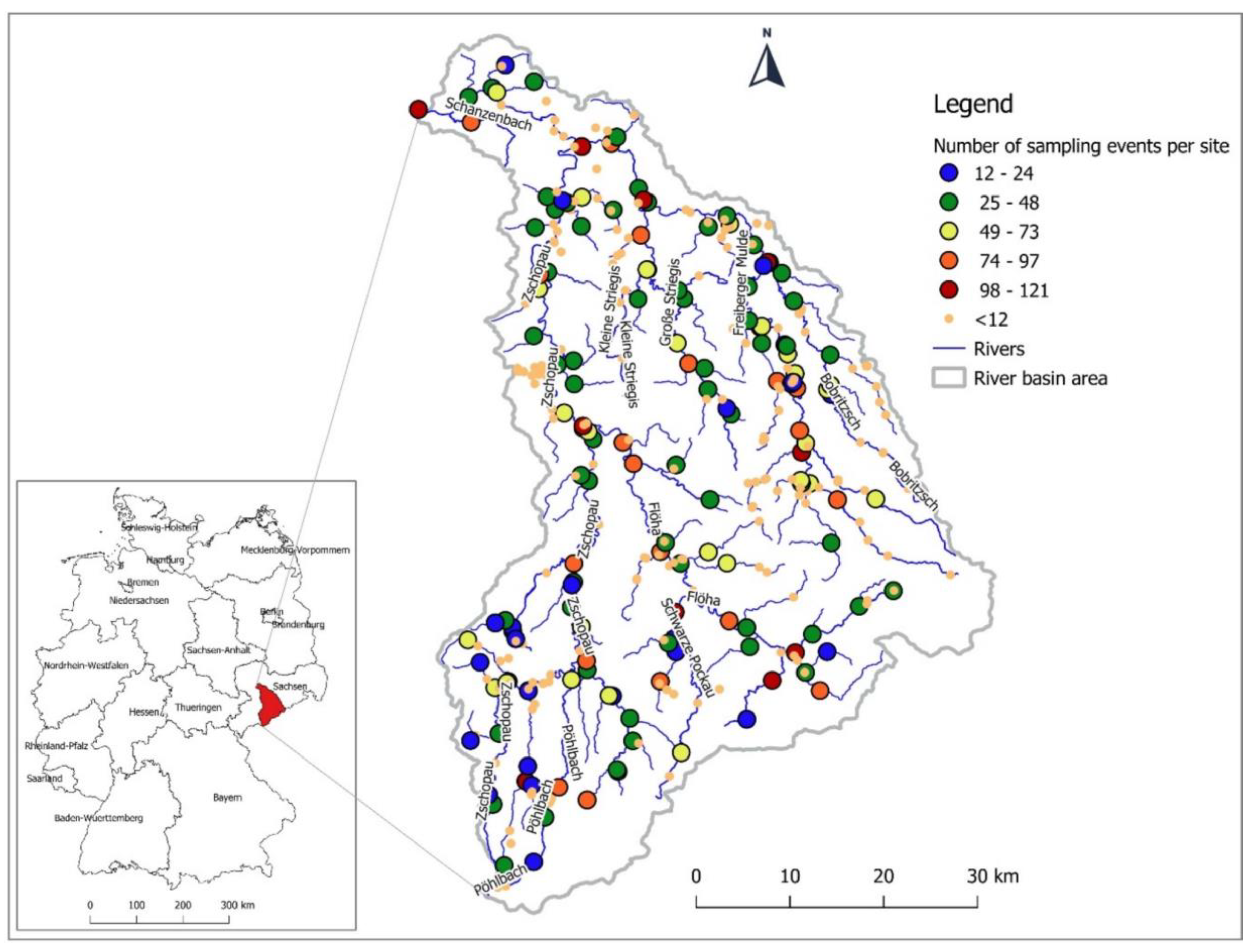
2.1. Study Area
2.2. Data Selection and Preparation
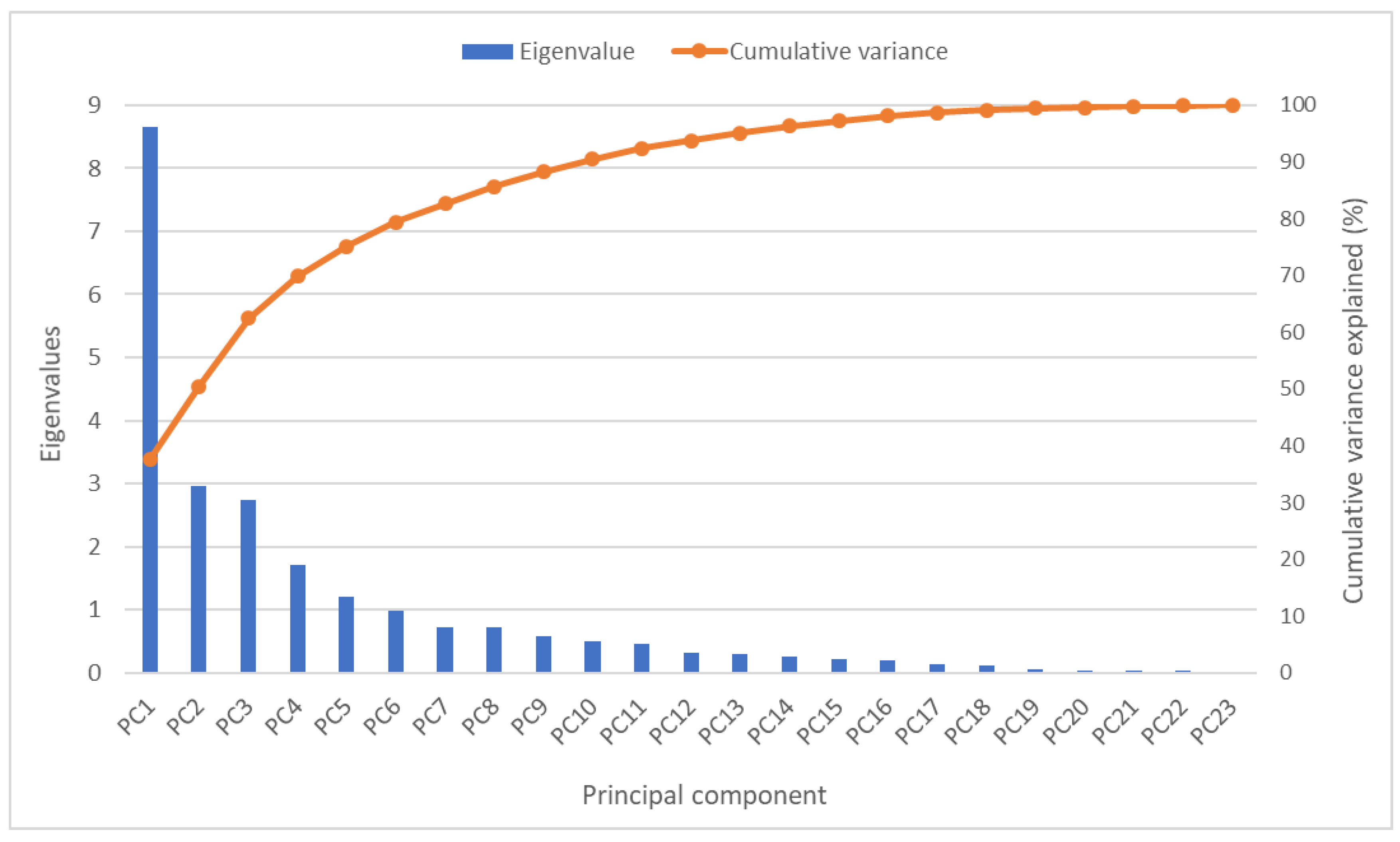
2.3. Principal Component Analysis
3. Results and Discussion
3.1. Data Screening and Descriptive Statistics
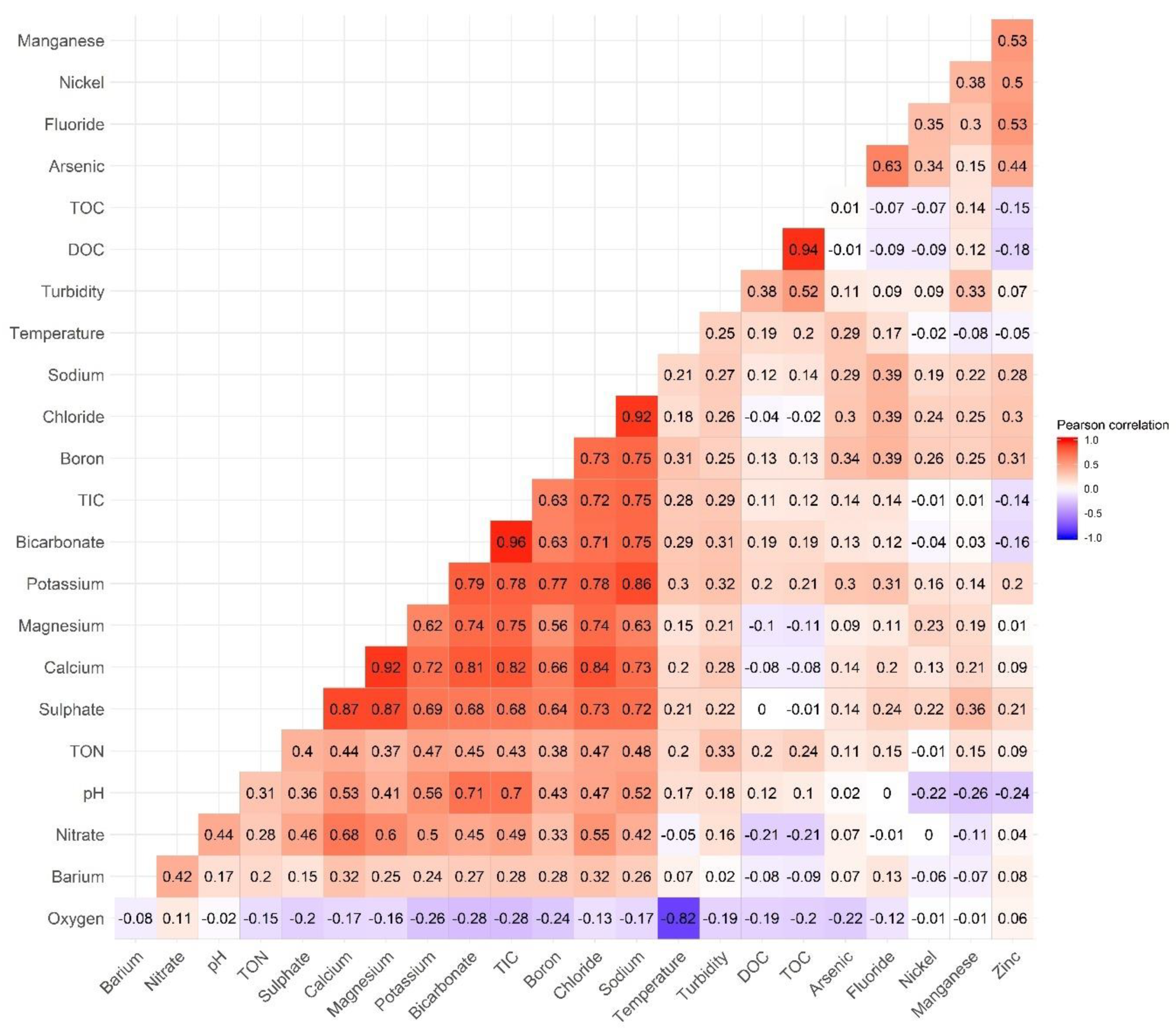
3.2. Characterized Water Quality Parameters and Sources Identification Based on Factor Loadings
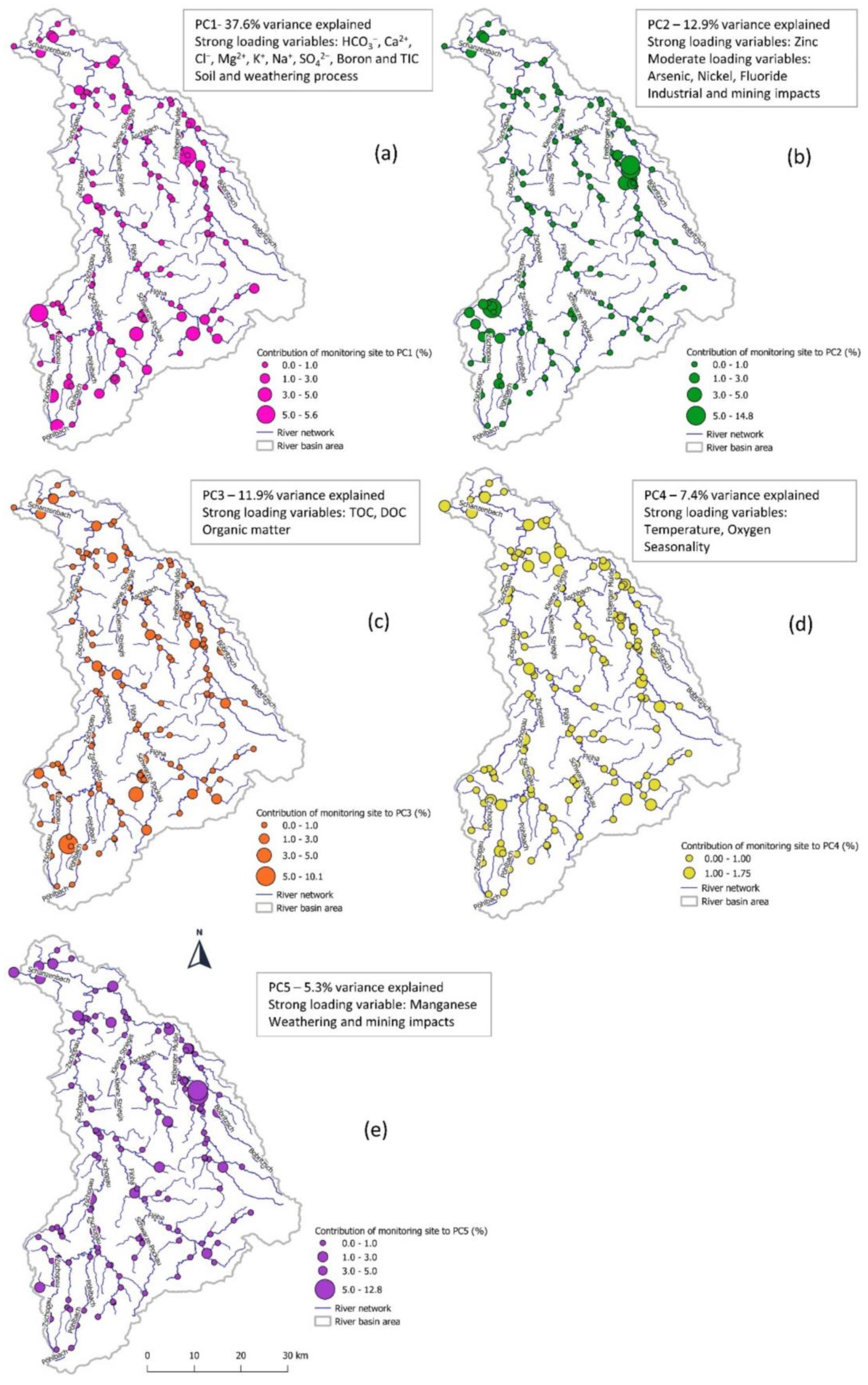
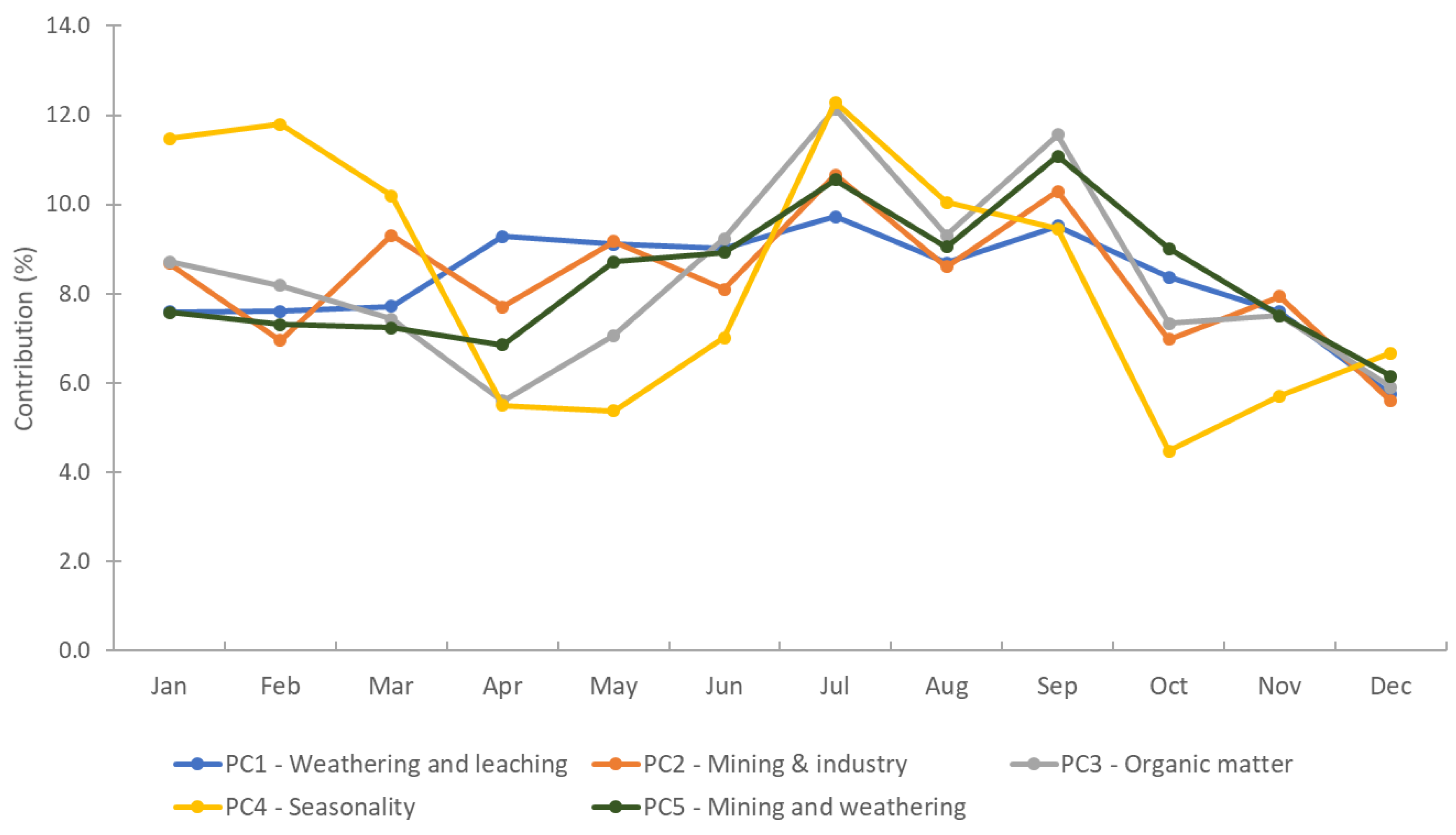
3.3. Spatial and Temporal Variability of Water Quality Based on the Contribution of Observations
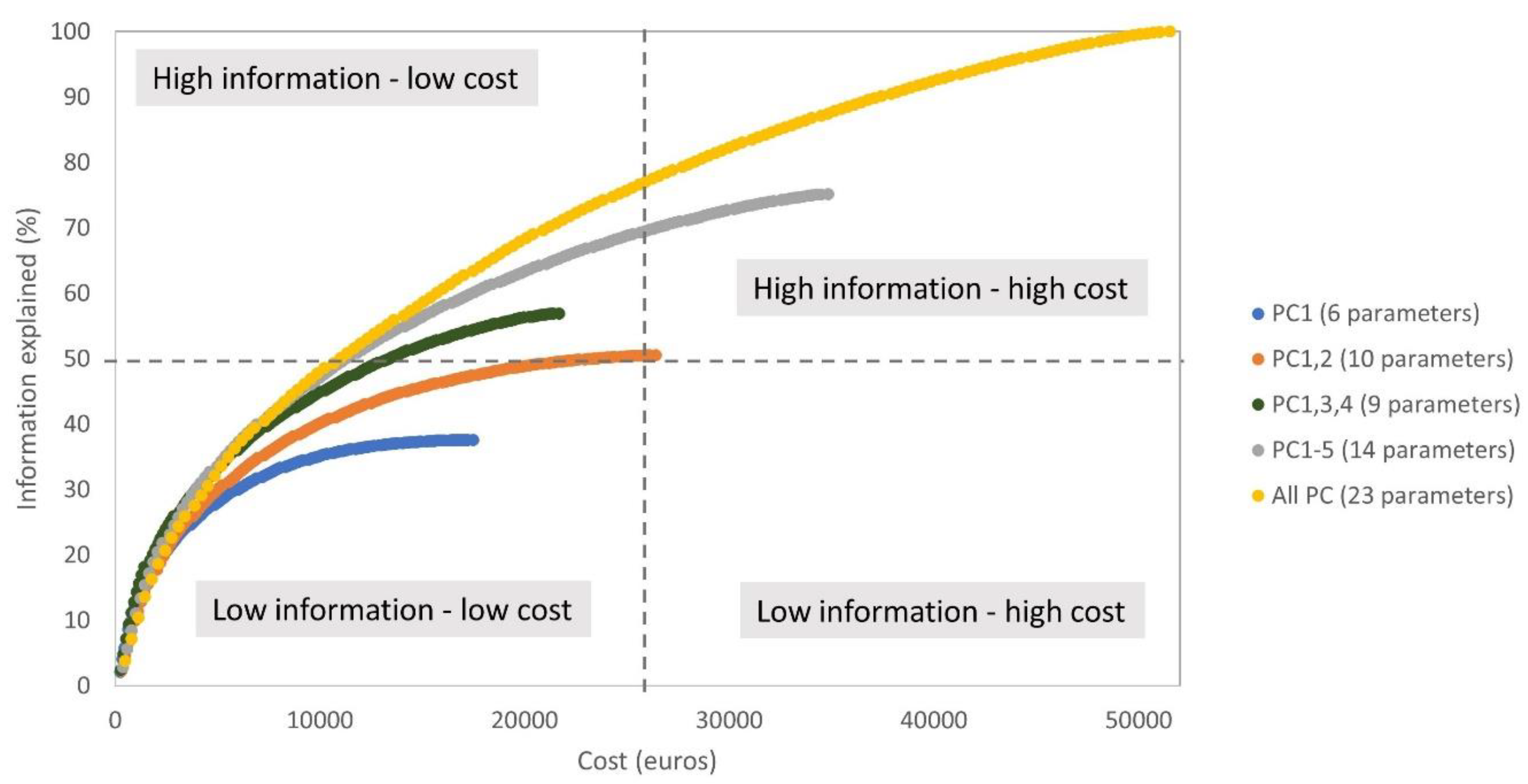
3.4. Cost-Effectiveness of Proposed Water Quality Monitoring Network Based on PCA Results
- PC1: monitoring of six variables strongly correlated to PC1 (Ca2+, Cl−, K+, SO42−, Boron, and TIC) and obtaining 37.6% of information accordingly;
- PC1,2: monitoring of 10 variables strongly correlated to PC1 and PC2 (Ca2+, Cl−, K+, SO42−, Boron, TIC, Fluoride, Arsenic, Zinc, Nickel) and obtaining 50.5% of information accordingly;
- PC1,3,4: monitoring of nine variables strongly correlated to PC1, PC3, and PC4 (Ca2+, Cl−, K+, SO42−, Boron, TIC, TOC, temperature, oxygen) and obtaining 56.9% of information accordingly;
- PC1-5: monitoring of 14 variables correlated to the first five components (Ca2+, Cl−, K+, SO42−, Boron, TIC, Fluoride, Arsenic, Zinc, Nickel, TOC, Oxygen, Temperature, Manganese) and obtaining 75.1% of information accordingly; and
- All PC: monitoring of all 23 variables and obtaining 100% of the information.
4. Conclusions
Author Contributions
Funding
Acknowledgments
Conflicts of Interest
Appendix A

| Site | River | PC1 | PC2 | PC3 | PC4 | PC5 | PC1,2 | PC1,3,4 | PC1-5 | All PCs |
|---|---|---|---|---|---|---|---|---|---|---|
| OBF31301 | Freiberger Mulde | 0.206 | 0.015 | 0.125 | 0.092 | 0.059 | 0.222 | 0.424 | 0.498 | 0.689 |
| OBF31302 | Zethaubach | 0.066 | 0.037 | 0.054 | 0.032 | 0.004 | 0.102 | 0.151 | 0.192 | 0.283 |
| OBF31303 | Helbigsdorfer Bach | 0.032 | 0.078 | 0.037 | 0.048 | 0.009 | 0.110 | 0.117 | 0.205 | 0.296 |
| OBF31400 | Freiberger Mulde | 0.081 | 0.041 | 0.076 | 0.043 | 0.036 | 0.122 | 0.200 | 0.277 | 0.422 |
| OBF31500 | Freiberger Mulde | 0.094 | 0.011 | 0.053 | 0.036 | 0.040 | 0.105 | 0.183 | 0.234 | 0.573 |
| OBF31510 | Freiberger Mulde | 0.156 | 0.059 | 0.052 | 0.030 | 0.046 | 0.215 | 0.238 | 0.343 | 0.650 |
| OBF31520 | Freiberger Mulde | 0.042 | 0.039 | 0.012 | 0.009 | 0.010 | 0.081 | 0.063 | 0.112 | 0.182 |
| OBF31530 | Stangenbergbach | 0.075 | 0.220 | 0.042 | 0.012 | 0.045 | 0.295 | 0.130 | 0.395 | 0.544 |
| OBF31540 | Hüttenbach | 0.312 | 0.069 | 0.071 | 0.032 | 0.038 | 0.381 | 0.415 | 0.522 | 0.793 |
| OBF31600 | Freiberger Mulde | 0.181 | 0.198 | 0.037 | 0.040 | 0.027 | 0.379 | 0.258 | 0.483 | 0.806 |
| OBF31601 | Kleinwaltersdorfer Bach | 0.020 | 0.011 | 0.023 | 0.056 | 0.010 | 0.031 | 0.100 | 0.121 | 0.213 |
| OBF31610 | Freiberger Mulde | 0.212 | 0.073 | 0.019 | 0.023 | 0.035 | 0.285 | 0.255 | 0.362 | 0.429 |
| OBF31700 | Freiberger Mulde | 0.739 | 0.255 | 0.070 | 0.070 | 0.112 | 0.994 | 0.880 | 1.246 | 1.510 |
| OBF31701 | Freiberger Mulde | 0.178 | 0.049 | 0.017 | 0.008 | 0.028 | 0.227 | 0.204 | 0.281 | 0.333 |
| OBF31710 | Freiberger Mulde | 0.215 | 0.039 | 0.028 | 0.017 | 0.029 | 0.253 | 0.260 | 0.328 | 0.395 |
| OBF31711 | Pitzschebach | 0.151 | 0.013 | 0.057 | 0.089 | 0.118 | 0.164 | 0.298 | 0.428 | 0.686 |
| OBF31800 | Freiberger Mulde | 0.189 | 0.035 | 0.021 | 0.024 | 0.023 | 0.224 | 0.233 | 0.291 | 0.346 |
| OBF31801 | Marienbach | 0.178 | 0.035 | 0.043 | 0.045 | 0.041 | 0.212 | 0.266 | 0.342 | 0.442 |
| OBF31900 | Freiberger Mulde | 0.195 | 0.034 | 0.022 | 0.024 | 0.022 | 0.229 | 0.241 | 0.297 | 0.358 |
| OBF31950 | Freiberger Mulde | 0.182 | 0.029 | 0.029 | 0.031 | 0.015 | 0.211 | 0.241 | 0.285 | 0.357 |
| OBF32000 | Freiberger Mulde | 0.462 | 0.065 | 0.070 | 0.076 | 0.038 | 0.527 | 0.608 | 0.711 | 0.859 |
| OBF32001 | Gärtitzer Bach | 0.598 | 0.083 | 0.043 | 0.074 | 0.063 | 0.682 | 0.715 | 0.862 | 1.005 |
| OBF32201 | Görnitzbach | 0.790 | 0.247 | 0.170 | 0.086 | 0.059 | 1.036 | 1.046 | 1.351 | 1.571 |
| OBF32202 | Schickelsbach | 0.347 | 0.062 | 0.075 | 0.036 | 0.042 | 0.409 | 0.458 | 0.562 | 0.690 |
| OBF32203 | Polkenbach | 0.559 | 0.143 | 0.050 | 0.063 | 0.045 | 0.702 | 0.672 | 0.860 | 0.991 |
| OBF32204 | Polkenbach | 0.334 | 0.055 | 0.019 | 0.047 | 0.052 | 0.389 | 0.399 | 0.507 | 0.598 |
| OBF32205 | Fritzschenbach | 0.365 | 0.064 | 0.073 | 0.072 | 0.070 | 0.429 | 0.511 | 0.645 | 0.778 |
| OBF32206 | Schanzenbach | 0.493 | 0.232 | 0.217 | 0.088 | 0.086 | 0.726 | 0.798 | 1.117 | 1.299 |
| OBF32300 | Freiberger Mulde | 0.251 | 0.032 | 0.092 | 0.092 | 0.057 | 0.282 | 0.434 | 0.523 | 0.742 |
| OBF32600 | Chemnitzbach | 0.079 | 0.035 | 0.115 | 0.044 | 0.022 | 0.114 | 0.237 | 0.294 | 0.406 |
| OBF32601 | Voigtsdorfer Bach | 0.087 | 0.005 | 0.063 | 0.026 | 0.008 | 0.092 | 0.176 | 0.189 | 0.342 |
| OBF32700 | Grosshartmannsdorfer Bach | 0.064 | 0.110 | 0.096 | 0.081 | 0.011 | 0.175 | 0.242 | 0.363 | 0.568 |
| OBF32750 | Gimmlitz | 0.293 | 0.027 | 0.116 | 0.067 | 0.008 | 0.320 | 0.476 | 0.511 | 0.657 |
| OBF32800 | Gimmlitz | 0.100 | 0.048 | 0.105 | 0.043 | 0.015 | 0.148 | 0.249 | 0.312 | 0.452 |
| OBF32900 | Münzbach | 2.102 | 0.153 | 0.243 | 0.089 | 0.206 | 2.255 | 2.434 | 2.793 | 3.363 |
| OBF32901 | Münzbach | 0.223 | 0.391 | 0.157 | 0.063 | 0.045 | 0.613 | 0.442 | 0.878 | 1.398 |
| OBF32903 | Münzbach | 0.349 | 0.050 | 0.039 | 0.024 | 0.038 | 0.399 | 0.413 | 0.501 | 0.728 |
| OBF33010 | Roter Graben | 0.157 | 1.909 | 0.055 | 0.054 | 0.675 | 2.066 | 0.266 | 2.849 | 3.273 |
| OBF33020 | Roter Graben | 0.414 | 1.154 | 0.035 | 0.054 | 0.425 | 1.568 | 0.504 | 2.082 | 2.405 |
| OBF33090 | Bobritzsch | 0.033 | 0.003 | 0.245 | 0.103 | 0.017 | 0.036 | 0.381 | 0.401 | 0.699 |
| OBF33100 | Bobritzsch | 0.018 | 0.048 | 0.086 | 0.060 | 0.073 | 0.066 | 0.164 | 0.285 | 0.515 |
| OBF33111 | Dittmannsdorfer Bach | 0.180 | 0.040 | 0.066 | 0.046 | 0.005 | 0.219 | 0.291 | 0.336 | 0.465 |
| OBF33200 | Bobritzsch | 0.051 | 0.061 | 0.100 | 0.106 | 0.100 | 0.112 | 0.257 | 0.418 | 0.657 |
| OBF33300 | Sohrbach | 0.018 | 0.018 | 0.042 | 0.042 | 0.015 | 0.036 | 0.101 | 0.134 | 0.455 |
| OBF33400 | Colmnitzbach | 0.023 | 0.017 | 0.033 | 0.048 | 0.020 | 0.040 | 0.105 | 0.142 | 0.234 |
| OBF33500 | Rodelandbach | 0.039 | 0.015 | 0.071 | 0.061 | 0.007 | 0.054 | 0.170 | 0.193 | 0.319 |
| OBF33601 | Erbisdorfer Wasser | 0.046 | 0.063 | 0.058 | 0.035 | 0.007 | 0.109 | 0.139 | 0.210 | 0.350 |
| OBF33650 | Grosse Striegis | 0.007 | 0.064 | 0.052 | 0.005 | 0.093 | 0.071 | 0.065 | 0.222 | 0.296 |
| OBF33701 | Oberreichenbacher Bach | 0.025 | 0.031 | 0.059 | 0.043 | 0.019 | 0.055 | 0.126 | 0.176 | 0.255 |
| OBF33702 | Schirmbach | 0.007 | 0.011 | 0.030 | 0.046 | 0.005 | 0.018 | 0.083 | 0.099 | 0.207 |
| OBF33703 | Kemnitzbach | 0.014 | 0.024 | 0.120 | 0.056 | 0.011 | 0.038 | 0.190 | 0.225 | 0.406 |
| OBF33710 | Grosse Striegis | 0.041 | 0.009 | 0.032 | 0.035 | 0.005 | 0.051 | 0.108 | 0.123 | 0.254 |
| OBF33711 | Langhennersdorfer Bach | 0.057 | 0.037 | 0.045 | 0.034 | 0.007 | 0.094 | 0.136 | 0.181 | 0.243 |
| OBF33713 | Aschbach | 0.058 | 0.029 | 0.027 | 0.068 | 0.037 | 0.088 | 0.154 | 0.220 | 0.468 |
| OBF33800 | Grosse Striegis | 0.096 | 0.012 | 0.061 | 0.066 | 0.008 | 0.108 | 0.223 | 0.243 | 0.422 |
| OBF33900 | Grosse Striegis | 0.249 | 0.027 | 0.085 | 0.093 | 0.010 | 0.276 | 0.427 | 0.464 | 0.676 |
| OBF34101 | Pahlbach | 0.043 | 0.025 | 0.037 | 0.035 | 0.028 | 0.069 | 0.116 | 0.169 | 0.287 |
| OBF34200 | Kleine Striegis | 0.178 | 0.054 | 0.034 | 0.056 | 0.006 | 0.232 | 0.267 | 0.328 | 0.425 |
| OBF34300 | Klatschbach | 0.506 | 0.104 | 0.085 | 0.107 | 0.015 | 0.611 | 0.698 | 0.818 | 1.219 |
| OBF34390 | Geyerbach | 0.271 | 0.340 | 0.006 | 0.006 | 0.050 | 0.611 | 0.283 | 0.673 | 0.831 |
| OBF34400 | Zschopau | 1.173 | 0.049 | 0.097 | 0.022 | 0.023 | 1.222 | 1.292 | 1.364 | 1.553 |
| OBF34401 | Geyerbach | 0.158 | 0.338 | 0.057 | 0.058 | 0.013 | 0.496 | 0.273 | 0.625 | 0.719 |
| OBF34403 | Greifenbach | 0.271 | 0.165 | 0.052 | 0.083 | 0.012 | 0.437 | 0.407 | 0.584 | 0.699 |
| OBF34404 | Greifenbach | 1.937 | 0.322 | 0.326 | 0.021 | 0.039 | 2.258 | 2.283 | 2.644 | 3.170 |
| OBF34405 | Zschopau | 0.203 | 0.015 | 0.028 | 0.008 | 0.009 | 0.218 | 0.239 | 0.262 | 0.352 |
| OBF34409 | Zschopau | 0.043 | 0.038 | 0.043 | 0.030 | 0.013 | 0.081 | 0.117 | 0.167 | 0.260 |
| OBF34601 | Hüttenbach | 0.124 | 0.046 | 0.112 | 0.107 | 0.103 | 0.170 | 0.343 | 0.492 | 0.690 |
| OBF34700 | Zschopau | 0.016 | 0.013 | 0.026 | 0.022 | 0.011 | 0.029 | 0.064 | 0.088 | 0.135 |
| OBF34701 | Venusberger Dorfbach | 0.056 | 0.010 | 0.067 | 0.032 | 0.005 | 0.066 | 0.155 | 0.171 | 0.282 |
| OBF34710 | Zschopau | 0.006 | 0.007 | 0.016 | 0.014 | 0.009 | 0.013 | 0.036 | 0.053 | 0.079 |
| OBF34801 | Dittmannsdorfer Bach | 0.009 | 0.014 | 0.052 | 0.027 | 0.005 | 0.023 | 0.089 | 0.108 | 0.183 |
| OBF34802 | Schwarzbach | 0.010 | 0.010 | 0.085 | 0.028 | 0.040 | 0.021 | 0.124 | 0.174 | 0.272 |
| OBF34890 | Zschopau | 0.013 | 0.010 | 0.029 | 0.035 | 0.016 | 0.023 | 0.077 | 0.103 | 0.155 |
| OBF34900 | Zschopau | 0.024 | 0.025 | 0.058 | 0.050 | 0.022 | 0.049 | 0.132 | 0.179 | 0.287 |
| OBF34901 | Eubaer Bach | 0.382 | 0.020 | 0.052 | 0.046 | 0.007 | 0.403 | 0.479 | 0.507 | 0.673 |
| OBF34910 | Zschopau | 0.026 | 0.019 | 0.053 | 0.072 | 0.035 | 0.045 | 0.151 | 0.206 | 0.321 |
| OBF35001 | Mühlbach | 0.016 | 0.020 | 0.051 | 0.026 | 0.032 | 0.036 | 0.093 | 0.145 | 0.231 |
| OBF35002 | Lützelbach | 0.181 | 0.017 | 0.019 | 0.040 | 0.008 | 0.199 | 0.240 | 0.266 | 0.365 |
| OBF35003 | Holzbach | 0.132 | 0.013 | 0.036 | 0.034 | 0.013 | 0.146 | 0.203 | 0.229 | 0.308 |
| OBF35101 | Ottendorfer Bach | 0.097 | 0.028 | 0.038 | 0.046 | 0.011 | 0.125 | 0.181 | 0.220 | 0.306 |
| OBF35102 | Altmittweidaer Bach | 0.339 | 0.050 | 0.061 | 0.076 | 0.011 | 0.390 | 0.476 | 0.538 | 0.685 |
| OBF35103 | Auenbach | 0.103 | 0.048 | 0.036 | 0.041 | 0.010 | 0.151 | 0.180 | 0.239 | 0.320 |
| OBF35200 | Zschopau | 0.041 | 0.020 | 0.090 | 0.078 | 0.024 | 0.061 | 0.209 | 0.252 | 0.390 |
| OBF35251 | Schweikershainer Bach | 0.151 | 0.059 | 0.054 | 0.063 | 0.016 | 0.210 | 0.267 | 0.343 | 0.445 |
| OBF35252 | Richzenhainer Bach | 0.324 | 0.092 | 0.069 | 0.066 | 0.012 | 0.416 | 0.459 | 0.564 | 0.736 |
| OBF35253 | Richzenhainer Bach | 0.595 | 0.034 | 0.055 | 0.073 | 0.056 | 0.629 | 0.723 | 0.813 | 0.998 |
| OBF35254 | Gebersbach | 0.340 | 0.084 | 0.089 | 0.069 | 0.051 | 0.425 | 0.498 | 0.634 | 0.834 |
| OBF35255 | Eulitzbach | 0.374 | 0.059 | 0.137 | 0.089 | 0.094 | 0.433 | 0.599 | 0.752 | 1.012 |
| OBF35257 | Mortelbach | 0.222 | 0.072 | 0.028 | 0.030 | 0.006 | 0.294 | 0.280 | 0.358 | 0.456 |
| OBF35258 | Mortelbach | 0.182 | 0.027 | 0.055 | 0.096 | 0.048 | 0.209 | 0.333 | 0.408 | 0.688 |
| OBF35310 | Zschopau | 0.008 | 0.004 | 0.017 | 0.010 | 0.005 | 0.012 | 0.035 | 0.044 | 0.070 |
| OBF35350 | Zschopau | 0.075 | 0.063 | 0.137 | 0.130 | 0.042 | 0.138 | 0.341 | 0.447 | 0.683 |
| OBF35391 | Rote Pfütze | 0.007 | 0.119 | 0.025 | 0.016 | 0.149 | 0.126 | 0.047 | 0.315 | 0.445 |
| OBF35400 | Rote Pfütze | 0.110 | 0.009 | 0.077 | 0.041 | 0.008 | 0.119 | 0.228 | 0.245 | 0.358 |
| OBF35490 | Sehma | 1.355 | 0.013 | 0.088 | 0.057 | 0.020 | 1.368 | 1.500 | 1.533 | 1.736 |
| OBF35600 | Sehma | 0.100 | 0.024 | 0.025 | 0.019 | 0.003 | 0.124 | 0.143 | 0.171 | 0.223 |
| OBF35601 | Lampertsbach | 1.127 | 0.320 | 1.209 | 0.117 | 0.019 | 1.446 | 2.453 | 2.791 | 3.774 |
| OBF35602 | Lampertsbach | 0.119 | 0.007 | 0.007 | 0.009 | 0.003 | 0.125 | 0.135 | 0.145 | 0.216 |
| OBF35650 | Sehma | 0.046 | 0.020 | 0.014 | 0.007 | 0.003 | 0.066 | 0.067 | 0.090 | 0.142 |
| OBF35800 | Sehma | 0.070 | 0.036 | 0.056 | 0.064 | 0.053 | 0.106 | 0.190 | 0.279 | 0.572 |
| OBF35802 | Sehma | 0.102 | 0.193 | 0.023 | 0.077 | 0.003 | 0.295 | 0.201 | 0.397 | 0.565 |
| OBF36000 | Pöhlbach | 0.051 | 0.023 | 0.035 | 0.014 | 0.007 | 0.074 | 0.101 | 0.130 | 0.289 |
| OBF36100 | Pöhlbach | 0.031 | 0.007 | 0.021 | 0.014 | 0.009 | 0.038 | 0.066 | 0.081 | 0.207 |
| OBF36200 | Pöhlbach | 0.037 | 0.019 | 0.055 | 0.055 | 0.008 | 0.056 | 0.147 | 0.173 | 0.442 |
| OBF36300 | Pöhlbach | 0.026 | 0.012 | 0.058 | 0.035 | 0.007 | 0.038 | 0.119 | 0.138 | 0.266 |
| OBF36400 | Pressnitz | 1.101 | 0.015 | 0.078 | 0.031 | 0.048 | 1.116 | 1.210 | 1.274 | 1.572 |
| OBF36402 | Steinbach | 0.262 | 0.024 | 0.036 | 0.038 | 0.013 | 0.285 | 0.335 | 0.372 | 0.494 |
| OBF36403 | Haselbach | 0.384 | 0.011 | 0.024 | 0.028 | 0.004 | 0.394 | 0.436 | 0.450 | 0.629 |
| OBF36404 | Sandbach | 0.015 | 0.019 | 0.040 | 0.021 | 0.010 | 0.033 | 0.076 | 0.104 | 0.200 |
| OBF36450 | Pressnitz | 0.122 | 0.004 | 0.018 | 0.012 | 0.002 | 0.126 | 0.151 | 0.158 | 0.189 |
| OBF36500 | Pressnitz | 0.292 | 0.022 | 0.075 | 0.056 | 0.014 | 0.314 | 0.423 | 0.458 | 0.598 |
| OBF36600 | Jöhstädter Schwarzwasser | 0.553 | 0.023 | 0.047 | 0.039 | 0.015 | 0.575 | 0.639 | 0.677 | 0.952 |
| OBF36601 | Jöhstädter Schwarzwasser | 0.230 | 0.014 | 0.028 | 0.031 | 0.004 | 0.243 | 0.288 | 0.306 | 0.396 |
| OBF36700 | Rauschenbach | 0.118 | 0.029 | 0.079 | 0.028 | 0.014 | 0.147 | 0.225 | 0.268 | 0.435 |
| OBF36793 | Wilisch | 0.036 | 0.091 | 0.085 | 0.057 | 0.046 | 0.126 | 0.178 | 0.315 | 0.444 |
| OBF36794 | Wilisch | 0.131 | 0.874 | 0.032 | 0.060 | 0.010 | 1.004 | 0.224 | 1.107 | 1.469 |
| OBF36795 | Wilisch | 0.029 | 0.287 | 0.022 | 0.029 | 0.006 | 0.316 | 0.079 | 0.372 | 0.520 |
| OBF36797 | Wilisch | 0.015 | 0.062 | 0.048 | 0.031 | 0.017 | 0.077 | 0.094 | 0.173 | 0.238 |
| OBF36800 | Wilisch | 0.065 | 0.116 | 0.051 | 0.110 | 0.060 | 0.182 | 0.227 | 0.404 | 0.714 |
| OBF36801 | Jahnsbach | 0.022 | 0.017 | 0.066 | 0.040 | 0.006 | 0.039 | 0.127 | 0.151 | 0.259 |
| OBF36803 | Jahnsbach | 0.271 | 0.192 | 0.015 | 0.062 | 0.005 | 0.463 | 0.349 | 0.546 | 0.647 |
| OBF36850 | Flöha | 0.787 | 0.024 | 0.034 | 0.022 | 0.006 | 0.811 | 0.843 | 0.873 | 0.997 |
| OBF36911 | Cämmerswalder Dorfbach | 0.120 | 0.031 | 0.089 | 0.028 | 0.006 | 0.151 | 0.236 | 0.274 | 0.378 |
| OBF36912 | Mortelbach | 0.098 | 0.031 | 0.073 | 0.032 | 0.006 | 0.129 | 0.203 | 0.241 | 0.355 |
| OBF37000 | Flöha | 0.446 | 0.033 | 0.101 | 0.065 | 0.018 | 0.479 | 0.612 | 0.663 | 0.801 |
| OBF37001 | Rungstockbach | 0.509 | 0.009 | 0.023 | 0.028 | 0.021 | 0.518 | 0.560 | 0.590 | 0.721 |
| OBF37010 | Flöha | 0.236 | 0.015 | 0.057 | 0.049 | 0.011 | 0.251 | 0.342 | 0.368 | 0.499 |
| OBF37101 | Saidenbach | 0.064 | 0.055 | 0.026 | 0.022 | 0.018 | 0.120 | 0.112 | 0.185 | 0.266 |
| OBF37103 | Saidenbach | 0.064 | 0.079 | 0.058 | 0.046 | 0.020 | 0.143 | 0.168 | 0.267 | 0.359 |
| OBF37104 | Haselbach | 0.167 | 0.076 | 0.064 | 0.038 | 0.019 | 0.243 | 0.269 | 0.364 | 0.475 |
| OBF37105 | Lautenbach | 0.288 | 0.054 | 0.056 | 0.060 | 0.079 | 0.342 | 0.404 | 0.538 | 0.691 |
| OBF37106 | Röthenbach | 0.118 | 0.043 | 0.057 | 0.054 | 0.015 | 0.161 | 0.229 | 0.287 | 0.371 |
| OBF37300 | Flöha | 0.097 | 0.035 | 0.142 | 0.080 | 0.018 | 0.131 | 0.318 | 0.371 | 0.544 |
| OBF37400 | Schweinitz | 0.479 | 0.025 | 0.220 | 0.074 | 0.012 | 0.504 | 0.773 | 0.810 | 0.990 |
| OBF37401 | Seiffener Bach | 0.023 | 0.013 | 0.030 | 0.074 | 0.061 | 0.037 | 0.127 | 0.201 | 0.325 |
| OBF37404 | Seiffener Bach | 0.006 | 0.033 | 0.066 | 0.125 | 0.008 | 0.038 | 0.197 | 0.237 | 0.353 |
| OBF37450 | Natzschung | 0.300 | 0.003 | 0.030 | 0.013 | 0.002 | 0.303 | 0.343 | 0.349 | 0.390 |
| OBF37500 | Natzschung | 1.465 | 0.024 | 0.178 | 0.079 | 0.010 | 1.489 | 1.722 | 1.756 | 1.970 |
| OBF37600 | Bielabach | 0.039 | 0.049 | 0.043 | 0.025 | 0.009 | 0.089 | 0.107 | 0.165 | 0.251 |
| OBF37800 | Schwarze Pockau | 0.908 | 0.012 | 0.351 | 0.051 | 0.007 | 0.919 | 1.310 | 1.328 | 1.503 |
| OBF37910 | Schwarze Pockau | 1.196 | 0.022 | 0.423 | 0.089 | 0.009 | 1.219 | 1.708 | 1.740 | 1.976 |
| OBF38000 | Schwarze Pockau | 0.149 | 0.063 | 0.220 | 0.071 | 0.052 | 0.212 | 0.440 | 0.555 | 0.725 |
| OBF38100 | Rote Pockau | 0.024 | 0.033 | 0.084 | 0.025 | 0.046 | 0.057 | 0.133 | 0.212 | 0.300 |
| OBF38101 | Rote Pockau | 0.058 | 0.179 | 0.032 | 0.026 | 0.001 | 0.237 | 0.115 | 0.295 | 0.337 |
| OBF38190 | Rote Pockau | 0.001 | 0.118 | 0.013 | 0.032 | 0.006 | 0.118 | 0.046 | 0.170 | 0.210 |
| OBF38200 | Rote Pockau | 1.732 | 0.025 | 0.436 | 0.050 | 0.017 | 1.757 | 2.219 | 2.260 | 2.695 |
| OBF38201 | Schlettenbach | 0.088 | 0.015 | 0.020 | 0.034 | 0.034 | 0.103 | 0.143 | 0.192 | 0.305 |
| OBF38400 | Grosse Lössnitz | 0.019 | 0.080 | 0.097 | 0.052 | 0.019 | 0.099 | 0.168 | 0.266 | 0.477 |
| OBF38401 | Gahlenzer Bach | 0.025 | 0.027 | 0.049 | 0.045 | 0.022 | 0.052 | 0.120 | 0.169 | 0.304 |
| OBF38402 | Weissbach | 0.058 | 0.049 | 0.055 | 0.040 | 0.073 | 0.106 | 0.153 | 0.274 | 0.469 |
| OBF38500 | Hetzbach | 0.037 | 0.044 | 0.136 | 0.068 | 0.034 | 0.082 | 0.242 | 0.320 | 0.504 |
| Total variance explained (%) | 37.6 | 12.9 | 11.9 | 7.4 | 5.3 | 50.5 | 56.9 | 75.1 | 100 | |
References
- Singh:, K.P.; Malik, A.; Mohan, D.; Sinha, S. Multivariate statistical techniques for the evaluation of spatial and temporal variations in water quality of Gomti River (India)—A case study. Water Res. 2004, 38, 3980–3992. [Google Scholar] [CrossRef]
- UNEP. A Snapshot of the World’s Water Quality: Towards a Global Assessment; United Nations Environment Programme: Nairobi, Kenya, 2016; p. 162. [Google Scholar]
- Carpenter, S.R.; Caraco, N.F.; Correll, D.L.; Howarth, R.W.; Sharpley, A.N.; Smith, V.H. Nonpoint Pollution of Surface Waters with Phosphorus and Nitrogen. Ecol. Appl. 1998, 8, 559–568. [Google Scholar] [CrossRef]
- Arle, J.; Mohaupt, V.; Kirst, I. Monitoring of Surface Waters in Germany under the Water Framework Directive—A Review of Approaches, Methods and Results. Water 2016, 8, 217. [Google Scholar] [CrossRef]
- European Environment Agency Chemical Status of Surface Water Bodies. Available online: https://www.eea.europa.eu/themes/water/european-waters/water-quality-and-water-assessment/water-assessments/chemical-status-of-surface-water-bodies (accessed on 3 January 2020).
- Sanders, T.G. Design of Networks for Monitoring Water Quality; Water Resources Publication: Colorado, CO, USA, 1983. [Google Scholar]
- United Nations, World Health Organization. Water Quality Monitoring: A Practical Guide to the Design and Implementation of Freshwater Quality Studies and Monitoring Programmes, 1st ed.; Bartram, J., Ballance, R., Eds.; E & FN Spon: London, UK; New York, NY, USA, 1996; ISBN 978-0-419-22320-7. [Google Scholar]
- Ward, R.C.; Loftis, J.C.; McBride, G.B. The “Data rich but Information-poor” Syndrome in Water Quality Monitoring. Environ. Manag. 1986, 10, 291–297. [Google Scholar] [CrossRef]
- Dixon, W.; Chiswell, B. Review of aquatic monitoring program design. Water Res. 1996, 30, 1935–1948. [Google Scholar] [CrossRef]
- Harmancioglu, N.B.; Alpaslan, N. Water quality monitoring network design: A problem of multi-objective decision making. JAWRA J. Am. Water Resour. Assoc. 1992, 28, 179–192. [Google Scholar] [CrossRef]
- Behmel, S.; Damour, M.; Ludwig, R.; Rodriguez, M.J. Water quality monitoring strategies—A review and future perspectives. Sci. Total Environ. 2016, 571, 1312–1329. [Google Scholar] [CrossRef]
- Strobl, R.O.; Robillard, P.D. Network design for water quality monitoring of surface freshwaters: A review. J. Environ. Manag. 2008, 87, 639–648. [Google Scholar] [CrossRef]
- Singh, K.P.; Basant, A.; Malik, A.; Jain, G. Artificial neural network modeling of the river water quality—A case study. Ecol. Model. 2009, 220, 888–895. [Google Scholar] [CrossRef]
- Pérez, C.J.; Vega-Rodríguez, M.A.; Reder, K.; Flörke, M. A Multi-Objective Artificial Bee Colony-based optimization approach to design water quality monitoring networks in river basins. J. Clean. Prod. 2017, 166, 579–589. [Google Scholar] [CrossRef]
- Park, S.Y.; Choi, J.H.; Wang, S.; Park, S.S. Design of a water quality monitoring network in a large river system using the genetic algorithm. Ecol. Model. 2006, 199, 289–297. [Google Scholar] [CrossRef]
- Puri, D.; Borel, K.; Vance, C.; Karthikeyan, R. Optimization of a Water Quality Monitoring Network Using a Spatially Referenced Water Quality Model and a Genetic Algorithm. Water 2017, 9, 704. [Google Scholar] [CrossRef] [Green Version]
- Couto, C.M.C.M.; Ribeiro, C.; Maia, A.; Santos, M.; Tiritan, M.E.; Ribeiro, A.R.; Pinto, E.; Almeida, A. Assessment of Douro and Ave River (Portugal) lower basin water quality focusing on physicochemical and trace element spatiotemporal changes. J. Environ. Sci. Health Part A 2018, 0, 1–11. [Google Scholar] [CrossRef] [PubMed]
- Nguyen, T.H.; Helm, B.; Hettiarachchi, H.; Caucci, S.; Krebs, P. The selection of design methods for river water quality monitoring networks: A review. Environ. Earth Sci. 2019, 78. [Google Scholar] [CrossRef]
- Abdi, H.; Williams, L.J. Principal component analysis. Wiley Interdiscip. Rev. Comput. Stat. 2010, 2, 433–459. [Google Scholar] [CrossRef]
- Vega, M.; Pardo, R.; Barrado, E.; Debán, L. Assessment of seasonal and polluting effects on the quality of river water by exploratory data analysis. Water Res. 1998, 32, 3581–3592. [Google Scholar] [CrossRef]
- Simeonov, V.; Stratis, J.A.; Samara, C.; Zachariadis, G.; Voutsa, D.; Anthemidis, A.; Sofoniou, M.; Kouimtzis, T. Assessment of the surface water quality in Northern Greece. Water Res. 2003, 37, 4119–4124. [Google Scholar] [CrossRef]
- Singh, K.P.; Malik, A.; Sinha, S. Water quality assessment and apportionment of pollution sources of Gomti river (India) using multivariate statistical techniques—a case study. Anal. Chim. Acta 2005, 538, 355–374. [Google Scholar] [CrossRef]
- Zhang, X.; Wang, Q.; Liu, Y.; Wu, J.; Yu, M. Application of multivariate statistical techniques in the assessment of water quality in the Southwest New Territories and Kowloon, Hong Kong. Environ. Monit. Assess. 2011, 173, 17–27. [Google Scholar] [CrossRef]
- Kim, M.; Kim, Y.; Kim, H.; Piao, W.; Kim, C. Enhanced monitoring of water quality variation in Nakdong River downstream using multivariate statistical techniques. Desalination Water Treat. 2016, 57, 12508–12517. [Google Scholar] [CrossRef]
- Calazans, G.M.; Pinto, C.C.; da Costa, E.P.; Perini, A.F.; Oliveira, S.C. Using multivariate techniques as a strategy to guide optimization projects for the surface water quality network monitoring in the Velhas river basin, Brazil. Environ. Monit. Assess. 2018, 190, 726. [Google Scholar] [CrossRef] [PubMed]
- Pinto, C.C.; Calazans, G.M.; Oliveira, S.C. Assessment of spatial variations in the surface water quality of the Velhas River Basin, Brazil, using multivariate statistical analysis and nonparametric statistics. Environ. Monit. Assess. 2019, 191, 164. [Google Scholar] [CrossRef] [PubMed]
- Peña-Guzmán, C.A.; Soto, L.; Diaz, A. A Proposal for Redesigning the Water Quality Network of the Tunjuelo River in Bogotá, Colombia through a Spatio-Temporal Analysis. Resources 2019, 8, 64. [Google Scholar] [CrossRef] [Green Version]
- Ouyang, Y. Evaluation of river water quality monitoring stations by principal component analysis. Water Res. 2005, 39, 2621–2635. [Google Scholar] [CrossRef]
- Wang, Y.B.; Liu, C.W.; Liao, P.Y.; Lee, J.J. Spatial pattern assessment of river water quality: Implications of reducing the number of monitoring stations and chemical parameters. Environ. Monit. Assess. 2014, 186, 1781–1792. [Google Scholar] [CrossRef]
- Greif, A. The impact of mining activities in the Ore Mountains on the Mulde river catchment upstream of the Mulde reservoir lake. Hydrol. Wasserbewirtsch. 2015, 59, 318–331. [Google Scholar]
- Klemm, W.; Greif, A.; Broekaert, J.A.C.; Siemens, V.; Junge, F.W.; van der Veen, A.; Schultze, M.; Duffek, A. A Study on Arsenic and the Heavy Metals in the Mulde River System. Acta Hydrochim. Hydrobiol. 2005, 33, 475–491. [Google Scholar] [CrossRef]
- Dimmer, R. Gewässergütedaten. Available online: https://www.umwelt.sachsen.de/umwelt/wasser/7112.htm (accessed on 28 June 2019).
- US EPA. Guidance for Data Quality Assessment-Practical Methods for Data Analysis; United States Environmental Protection Agency: Washington, WA, USA, 2000.
- Löwig, M. Geodatendownload des Fachbereichs Wasser. Available online: https://www.umwelt.sachsen.de/umwelt/wasser/10002.htm?data=beschaffenheit (accessed on 18 June 2019).
- Hubert, M.; Reynkens, T.; Schmitt, E.; Verdonck, T. Sparse PCA for High-Dimensional Data with Outliers. Technometrics 2016, 58, 424–434. [Google Scholar] [CrossRef]
- Odom, K.R. Assessment and redesign of the synoptic water quality monitoring network in the Great Smoky Mountains National Park. Ph.D. Thesis, University of Tennessee, Knoxville, Tennessee, 2003. [Google Scholar]
- Guigues, N.; Desenfant, M.; Hance, E. Combining multivariate statistics and analysis of variance to redesign a water quality monitoring network. Environ. Sci. Process. Impacts 2013, 15, 1692. [Google Scholar] [CrossRef]
- Shrestha, S.; Kazama, F. Assessment of surface water quality using multivariate statistical techniques: A case study of the Fuji river basin, Japan. Environ. Model. Softw. 2007, 22, 464–475. [Google Scholar] [CrossRef]
- Revelle, W. Psych: Procedures for Psychological, Psychometric, and Personality Research; 2019; Software; Available online: https://cran.r-project.org/web/packages/psych/index.html (accessed on 8 January 2020).
- Husson, F.; Josse, J.; Le, S.; Mazet, J.; Husson, M.F. Package ‘FactoMineR.’. In Package FactorMineR; 2019; Software; Available online: http://factominer.free.fr/.
- QGIS Development Team. QGIS Geographic Information System; Open Source Geospatial Foundation Project, 2019; Software; Available online: https://www.qgis.org/en/site/.
- LAWA German Guidance Document for the Implementation of the EC Water Framework Directive; Bund/Länder-Arbeitsgemeinschaft Wasser: Berlin, Germany, 2003.
- Meybeck, M. Global occurrence of major elements in rivers. Treatise Geochem. 2003, 5, 207–223. [Google Scholar]
- Salomons, W.; Förstner, U. Metals in the Hydrocycle; Springer: Berlin/Heidelberg, Germany, 1984; ISBN 978-3-642-69327-4. [Google Scholar]
- Imai, A.; Fukushima, T.; Matsushige, K.; Hwan Kim, Y. Fractionation and characterization of dissolved organic matter in a shallow eutrophic lake, its inflowing rivers, and other organic matter sources. Water Res. 2001, 35, 4019–4028. [Google Scholar] [CrossRef]
- Kump, L.R.; Brantley, S.L.; Arthur, M.A. Chemical weathering, atmospheric CO2, and climate. Annu. Rev. Earth Planet. Sci. 2000, 28, 611–667. [Google Scholar] [CrossRef] [Green Version]
- Landeslabor Berlin-Brandenburg Leistungs-verzeichnis. Available online: https://www.landeslabor.berlin-brandenburg.de/sixcms/detail.php/883783 (accessed on 10 November 2019).


| Parameter | Unit | Mean | SD | Median | Min | Max | Skew | Kurtosis | Censor Data (%) |
|---|---|---|---|---|---|---|---|---|---|
| Arsenic | µg/L | 7.69 | 26.62 | 2 | 0.21 | 480 | 9.84 | 117.64 | 3 |
| Barium | µg/L | 50.76 | 25.46 | 46 | 3 | 480 | 6.22 | 82.29 | 0 |
| Bicarbonate (HCO3−) | mg/L | 55.34 | 52.23 | 39 | 0 | 560 | 2.67 | 9.98 | 3.1 |
| Boron | µg/L | 32.87 | 46.36 | 22 | 2.83 | 1000 | 7.81 | 91.14 | 0.4 |
| Calcium (Ca2+) | mg/L | 30.62 | 22.37 | 25 | 2.1 | 180 | 2.13 | 5.75 | 0 |
| Chloride (Cl−) | mg/L | 31.21 | 33.53 | 23 | 1.1 | 1500 | 13.24 | 497.14 | 0 |
| Dissolved organic carbon (DOC) | mg/L | 3.74 | 3.02 | 3.1 | 0.35 | 65 | 6.32 | 68.79 | 0.5 |
| Fluoride | mg/L | 0.26 | 0.36 | 0.2 | 0.04 | 10 | 9.1 | 140.36 | 1.09 |
| Magnesium (Mg2+) | mg/L | 7.8 | 5.23 | 6.2 | 0.8 | 50 | 2.14 | 5.41 | 0 |
| Manganese | µg/L | 98.85 | 523.2 | 20 | 0.71 | 8400 | 9.62 | 101.35 | 0.5 |
| Nickel | µg/L | 3.56 | 6.23 | 2.2 | 0.35 | 95 | 6.12 | 44.76 | 6.1 |
| Nitrate (NO3−) | mg/L | 20.12 | 12.63 | 18.5 | 0.49 | 100 | 0.68 | 0.23 | 0 |
| Oxygen | mg/L | 10.86 | 1.51 | 10.7 | 2.3 | 16.9 | −0.08 | 0.71 | 0 |
| pH | (-) | 7.36 | 0.5 | 7.4 | 4.3 | 9.8 | −1.7 | 6.9 | 0 |
| Potassium (K+) | mg/L | 4.53 | 6.59 | 3.4 | 0.4 | 360 | 24.15 | 1146.83 | 0 |
| Sodium (Na+) | mg/L | 20.65 | 26.67 | 15 | 1.2 | 1000 | 10.67 | 268.96 | 0 |
| Sulphate (SO42−) | mg/L | 51.5 | 40.49 | 39 | 7 | 550 | 3.81 | 21.85 | 0 |
| Temperature | °C | 9.36 | 4.99 | 9.4 | −1.1 | 26.4 | 0.14 | -0.75 | 0 |
| Total inorganic carbon (TIC) | mg/L | 9.62 | 9.92 | 6.45 | 0.35 | 100 | 2.72 | 10.37 | 1.2 |
| Total organic carbon (TOC) | mg/L | 4.63 | 4.66 | 3.7 | 0.35 | 120 | 9.12 | 149.02 | 0.3 |
| Total organic nitrogen (TON) | mg/L | 0.9 | 0.87 | 0.6 | 0.07 | 15 | 2.73 | 17.05 | 9.3 |
| Turbidity | TE/F | 7.87 | 25.45 | 3.4 | 0 | 1100 | 22.91 | 781.86 | 0.6 |
| Zinc | µg/L | 187.9 | 1203.27 | 13 | 2.12 | 21000 | 11.05 | 140.11 | 6.4 |
| Parameters | PCA | Varimax-Rotated PCA | ||||||||
|---|---|---|---|---|---|---|---|---|---|---|
| PC1 | PC2 | PC3 | PC4 | PC5 | RC1 | RC3 | RC2 | RC5 | RC4 | |
| Arsenic | 0.31 | −0.52 | −0.27 | 0.37 | 0.35 | 0.09 | 0.01 | 0.8 | 0.03 | 0.23 |
| Barium | 0.34 | 0.03 | 0.23 | 0.17 | 0.36 | 0.35 | −0.12 | 0.26 | −0.34 | −0.07 |
| Bicarbonate | 0.88 | 0.34 | 0.03 | 0.02 | −0.01 | 0.88 | 0.2 | −0.03 | −0.17 | 0.19 |
| Boron | 0.81 | −0.17 | −0.12 | 0.04 | 0.1 | 0.7 | 0.16 | 0.4 | 0.1 | 0.15 |
| Calcium | 0.91 | 0.03 | 0.25 | −0.06 | −0.19 | 0.95 | −0.08 | 0.01 | 0.13 | 0.08 |
| Chloride | 0.9 | −0.17 | 0.12 | −0.06 | 0.06 | 0.87 | 0.01 | 0.32 | 0.12 | −0.01 |
| DOC | 0.11 | 0.38 | −0.77 | −0.31 | 0.15 | −0.02 | 0.92 | −0.06 | −0.05 | 0.09 |
| Fluoride | 0.35 | −0.63 | −0.2 | 0.23 | 0.33 | 0.14 | −0.03 | 0.82 | 0.15 | 0.09 |
| Magnesium | 0.83 | 0.02 | 0.28 | −0.08 | −0.36 | 0.89 | −0.15 | −0.12 | 0.24 | 0.11 |
| Manganese | 0.22 | −0.55 | −0.32 | −0.44 | −0.34 | 0.13 | 0.22 | 0.18 | 0.81 | −0.09 |
| Nickel | 0.19 | −0.67 | −0.11 | −0.1 | −0.2 | 0.08 | −0.1 | 0.38 | 0.62 | 0.00 |
| Nitrate | 0.58 | 0.1 | 0.5 | −0.09 | 0.13 | 0.69 | −0.23 | 0.00 | −0.18 | −0.23 |
| Oxygen | −0.29 | −0.12 | 0.48 | −0.66 | 0.36 | −0.12 | −0.11 | −0.07 | −0.02 | −0.93 |
| pH | 0.6 | 0.47 | 0.17 | 0.02 | 0.29 | 0.66 | 0.16 | −0.04 | −0.49 | −0.02 |
| Potassium | 0.89 | 0.03 | −0.09 | 0.00 | 0.13 | 0.82 | 0.24 | 0.29 | −0.03 | 0.12 |
| Sodium | 0.89 | −0.09 | −0.03 | −0.07 | 0.15 | 0.82 | 0.18 | 0.35 | 0.05 | 0.02 |
| Sulphate | 0.84 | −0.11 | 0.11 | −0.12 | −0.35 | 0.84 | −0.03 | 0.01 | 0.36 | 0.13 |
| Temperature | 0.33 | 0.14 | −0.47 | 0.69 | −0.22 | 0.15 | 0.14 | 0.15 | −0.1 | 0.9 |
| TIC | 0.88 | 0.3 | 0.08 | 0.05 | −0.02 | 0.89 | 0.13 | −0.01 | −0.16 | 0.19 |
| TOC | 0.12 | 0.36 | −0.81 | −0.34 | 0.15 | −0.02 | 0.96 | −0.04 | −0.02 | 0.09 |
| TON | 0.55 | 0.1 | −0.17 | −0.14 | 0.12 | 0.5 | 0.33 | 0.13 | −0.02 | 0.01 |
| Turbidity | 0.38 | 0.09 | −0.5 | −0.29 | −0.07 | 0.28 | 0.6 | 0.01 | 0.23 | 0.1 |
| Zinc | 0.18 | −0.84 | −0.11 | −0.1 | 0.14 | 0.03 | −0.09 | 0.69 | 0.51 | −0.17 |
| Eigenvalue | 8.646 | 2.973 | 2.743 | 1.703 | 1.214 | 8.027 | 2.632 | 2.565 | 2.062 | 1.993 |
| Variance | 0.376 | 0.129 | 0.119 | 0.074 | 0.053 | 0.349 | 0.114 | 0.112 | 0.09 | 0.087 |
| Cumulative Variance | 0.376 | 0.505 | 0.624 | 0.698 | 0.751 | 0.349 | 0.463 | 0.575 | 0.665 | 0.751 |
| Items | Related Principal Component | Price (Euro) | Analytical Method | Price per Principal Component (Euro) | Variance Per Principal Component (%) | Information Per Price (%/Euro) |
|---|---|---|---|---|---|---|
| Total inorganic carbon | PC1 | 16.8 † | 64.6 | 37.6 | 0.58 | |
| Boron | PC1 | 19.7 | DIN EN ISO 17294-2 2005-02 (E 29) | |||
| Chloride, Sulphate, Calcium, Sodium, Potassium, Fluoride, Magnesium, Nitrate | PC1 | 28.1 * | DIN EN ISO 10304-1:2009-07 (D 20) | |||
| Arsenic | PC2 | 19.7 | DIN EN ISO 17294-2 2005-02 (E 29) | 59.1 | 12.9 | 0.22 |
| Zinc | PC2 | 19.7 | DIN EN ISO 17294-2 2005-02 (E 29) | |||
| Nickel | PC2 | 19.7 | DIN EN ISO 17294-2 2005-02 (E 29) | |||
| Total organic carbon | PC3 | 16.8 | DIN EN 12260:1996 (H 34)IN EN 1484: 1997-08 (H 3) | 16.8 | 11.9 | 0.71 |
| Temperature | PC4 | 1.9 | DIN 38404 Teil 4 (C4) | 10.9 | 7.4 | 0.68 |
| Oxygen | PC4 | 9 | EN 25814:1992 (G22) DIN 3840-G23 | |||
| Manganese | PC5 | 28.1 | DIN 38406-E Serie | 28.1 | 5.3 | 0.19 |
| First 5 PCs | 179.5 | 75.1 | 0.42 | |||
| pH | All PC | 9 | DIN 38404-5:2009-07 (C5) | 290 | 100 | 0.34 |
| Turbidity | All PC | 9 | DIN EN ISO 7027: 2000-04 | |||
| Barium | All PC | 19.7 | DIN EN ISO 17294-2 2005-02(E 29) | |||
| DOC | All PC | 35.4 | DIN EN 1484: 1997-08 (H 3) | |||
| Bicarbonate | All PC | 1.9 | DEV D8: 1971 | |||
| TON | All PC | 35.4 | DIN EN 1484: 1997-08 (H 3) | |||
| Transportation from 1 km to 100 km | 152 | |||||
| Sampling with basic efforts | 35.1 |
© 2020 by the authors. Licensee MDPI, Basel, Switzerland. This article is an open access article distributed under the terms and conditions of the Creative Commons Attribution (CC BY) license (http://creativecommons.org/licenses/by/4.0/).
Share and Cite
Nguyen, T.H.; Helm, B.; Hettiarachchi, H.; Caucci, S.; Krebs, P. Quantifying the Information Content of a Water Quality Monitoring Network Using Principal Component Analysis: A Case Study of the Freiberger Mulde River Basin, Germany. Water 2020, 12, 420. https://doi.org/10.3390/w12020420
Nguyen TH, Helm B, Hettiarachchi H, Caucci S, Krebs P. Quantifying the Information Content of a Water Quality Monitoring Network Using Principal Component Analysis: A Case Study of the Freiberger Mulde River Basin, Germany. Water. 2020; 12(2):420. https://doi.org/10.3390/w12020420
Chicago/Turabian StyleNguyen, Thuy Hoang, Björn Helm, Hiroshan Hettiarachchi, Serena Caucci, and Peter Krebs. 2020. "Quantifying the Information Content of a Water Quality Monitoring Network Using Principal Component Analysis: A Case Study of the Freiberger Mulde River Basin, Germany" Water 12, no. 2: 420. https://doi.org/10.3390/w12020420