Uncertainty Quantification of Landslide Generated Waves Using Gaussian Process Emulation and Variance-Based Sensitivity Analysis ^†

Abstract

Simulations of landslide generated waves (LGWs) are prone to high levels of uncertainty. Here we present a probabilistic sensitivity analysis of an LGW model. The LGW model was realised through a smooth particle hydrodynamics (SPH) simulator, which is capable of modelling fluids with complex rheologies and includes flexible boundary conditions. This LGW model has parameters defining the landslide, including its rheology, that contribute to uncertainty in the simulated wave characteristics. Given the computational expense of this simulator, we made use of the extensive uncertainty quantification functionality of the Dakota toolkit to train a Gaussian process emulator (GPE) using a dataset derived from SPH simulations. Using the emulator we conducted a variance-based decomposition to quantify how much each input parameter to the SPH simulation contributed to the uncertainty in the simulated wave characteristics. Our results indicate that the landslide’s volume and initial submergence depth contribute the most to uncertainty in the wave characteristics, while the landslide rheological parameters have a much smaller influence. When estimated run-up is used as the indicator for LGW hazard, the slope angle of the shore being inundated is shown to be an additional influential parameter. This study facilitates probabilistic hazard analysis of LGWs, because it reveals which source characteristics contribute most to uncertainty in terms of how hazardous a wave will be, thereby allowing computational resources to be focused on better understanding that uncertainty.

1. Introduction

Landslide generated waves (LGWs) can be extremely hazardous [1,2], and it is difficult to predict their location, time, and severity [3]. The severity of the hazard posed by an LGW depends on various wave characteristics which are closely linked to landslide’s dynamics and location [4]. Lab scale submarine landslide experiments show that initial landslide submergence and the angle of the slope down which it slides strongly affect the energy conversion between the sliding mass and the wave [5]. The characteristics of the landslide that likewise have a key effect on the wave characteristics are volume and initial acceleration [6]. Landslide rheology, slope angle, and the interaction between the slide and the seafloor, all tie in to the initial acceleration and deformation of the landslide, and therefore also affect wave generation.

An ideal LGW hazard analysis would incorporate all these landslide characteristics and geometric input parameters because they contribute to uncertainty in the simulation results. However, it is computationally prohibitive to include all those parameters in a numerical modelling investigation capable of producing a full probabilistic hazard assessment. Determining the extent to which each of the input parameters contributes to variance in the simulated wave characteristics is beneficial, since computational resources can then be focused on examining those parameters that cause the greatest variability in the outcome.

Our study aims to quantify the relative importance of the input parameters to the level of hazard posed by an LGW through probabilistic sensitivity analysis (PSA). Ideally, this will make the probabilistic hazard assessment process computationally cheaper in the future, because the parameters that have a relatively small contribution to variance of the simulated wave characteristics can be discounted, and uncertainty analyses can focus on the parameters that contribute more to uncertainty. For a review of the benefits of global sensitivity analyses such as this, for investigating uncertainty in earth system models, see [7].

Here we use Smooth Particle Hydrodynamics (SPH), which is a meshless Lagrangian numerical modelling technique [8], to simulate LGWs and investigate their associated sources of uncertainty. Our chosen SPH simulator [9] is able to represent complex landslide rheology and flexible boundary conditions. We use an idealised geometry and model the slide as a fluid with a Herschel-Bulkley rheology (i.e., a dense fluid with viscosity, yield strength, and an exponent to define shear thinning or thickening behaviour).

A probabilistic sensitivity analysis requires extensive sampling of the entire parameter space. This is infeasible using only the SPH simulator due to its high computational cost. To facilitate a richer sampling of the input parameter space we use Dakota [10], an extensive uncertainty quantification and optimisation toolkit, to train a Gaussian process emulator (GPE) with a training dataset of SPH simulation inputs and results. GPEs have been used previously both for LGW studies [11] and in other fields such as materials science [12] and climate modelling [13]. The Gaussian process emulator is tested against additional SPH simulation results to ensure that it is able to predict the simulated outcomes to a satisfactory degree of accuracy. We then use the emulator to extensively sample the input parameter space and quantify the uncertainty in the simulated wave characteristics. We use the samples from the emulator to calculate Sobol’ indices, which quantify the extent to which each input parameter is responsible for the variance in the output.

We also conduct a further investigation of the output parameter. Maximum wave amplitude is a widely-used metric of near-field wave hazard; however, alternative metrics may provide better hazard measures far from the source (e.g., after propagation across an ocean basin) [14]. Transoceanic tsunamis are especially hazardous because of their very long wavelength and the large volumes of water that spill on to the coast as a result. We therefore also investigate two other simulated output metrics: the positive displaced volume of the wave and an analytical approximation for the run-up height, which we refer to here as the run-up approximation. The latter adds two more input parameters to the sensitivity analysis beyond those investigated at the source. The results of the sensitivity analyses using different output metrics are then compared.

2. Methods

To summarise, a training data set was constructed using an idealised LGW scenario (Figure 1) and our chosen SPH simulator. The relevant input parameters and the bounds between which we drew samples were selected based on a literature review and previous work. The first simulated output parameter we chose to quantify how hazardous the LGW could be was the maximum wave amplitude. The GPE and variance-based decomposition were undertaken using Dakota [10]. The second output parameter we investigated, positive displaced volume in the wave, was also drawn from the results of the SPH simulations. The third output parameter was an approximation of run-up (Section 2.5.2), which was calculated based on the waves simulated in SPH and additional input parameters defining the geometry of the run-up region. The GPE and variance-based decomposition were repeated for the displaced volume and run-up approximation output parameters.

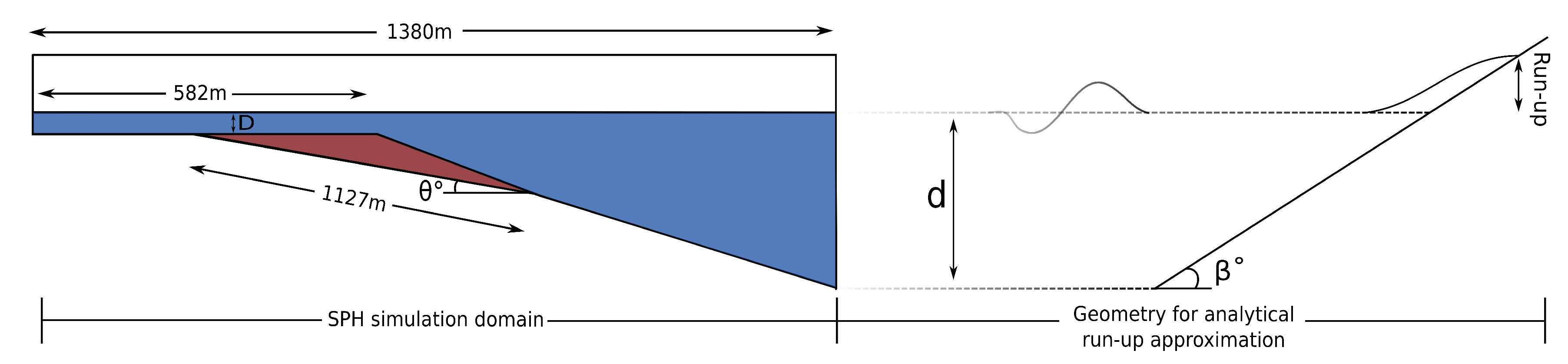
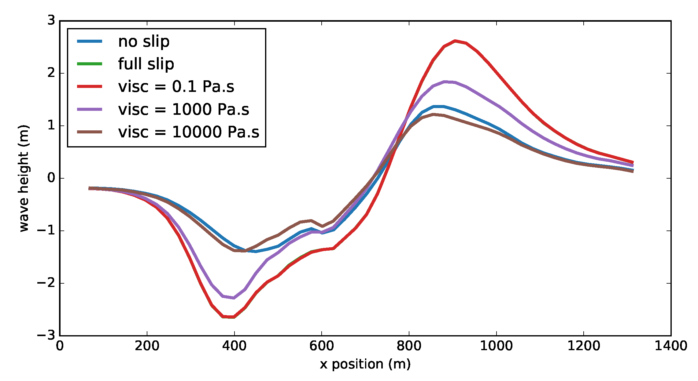
2.1. SPH Modelling of LGWs

Our LGW simulations were performed using a Smooth Particle Hydrodynamics (SPH) simulator [9,15]. The SPH numerical method discretises a fluid domain using evenly spaced free moving particles, and has been used in previous LGW studies [16,17,18,19]. Our chosen SPH simulator includes models for three rheology types:

• Newtonian: linear viscosity;
• Bingham: linear viscosity plus yield stress;
• Herschel-Bulkley: non-linear viscosity relationship plus yield stress.

Submarine landslides exhibit shear-thinning behaviour [20,21]. We, therefore, modelled the landslide rheology as a Herschel-Bulkley fluid in this work, which means there are four rheological parameters defining the landslide to consider during the PSA: density, viscosity, yield stress, and shear-thinning exponent.

Our SPH simulator also has a flexible boundary condition setting, which can be used to simulate the interaction of the base of the slide with the slope beneath. A single parameter is used to represent the viscosity of the boundary layer at the base of the slide and can span the range of boundary conditions between the extreme cases of no-slip and full-slip [15].

The other input parameters of importance in the LGW simulations are the slide volume, the initial submergence depth of the slide, and the slope angle.

2.2. Building the Training Dataset

In this work an idealised geometry is considered, as shown in Figure 1. The scale is based on landslide generated wave case studies from Alaskan bays [22,23]. Selecting the upper and lower bounds of each of the input parameters was achieved through a combination of model sensitivity tests and a literature review [11,20,23,24,25,26,27,28,29]. Parameter bounds are shown in

Table 1. Input parameter bounds. The first eight parameters pertain to the SPH simulations. The final two are used in the run-up approximation calculation described in Section 2.5.2.

Parameter	Lower Bound	Upper Bound
Submergence depth (D)	146.0 m	196.0 m
Viscosity ($\mu$)	1.0 Pa s	1000.0 Pa s
Yield stress ($\tau$)	0.0 Pa	20,000.0 Pa
Shear thinning exponent (N)	$0.33$	$1.0$
Density ($\rho$)	1800.0 kg m−3	2300.0 kg m−3
Slope angle—source ($\theta$)	0.5°	8.0°
Boundary layer viscosity/length scale ($\frac{\mu }{l}$)	0.2 kg m−2 s−1	20,000.0 kg m−2 s−1
Volume (V)	1839.75 m3	7347.25 m3
Open ocean water depth (d)	100 m	500 m
Slope angle—inundation ($\beta$)	0.5°	8.0°

.

The minimum submergence depth, D, was chosen so that the largest volume slide, at the shallowest slope angle, would not breach the water’s surface. The maximum submergence depth was this minimum submergence depth plus an additional water column of double the maximum slide thickness.

The bounds for viscosity were selected based on bounds considered in other numerical modelling studies [11,23,28]. The bounds for yield stress were likewise based on a literature review [11,27,29] and sensitivity tests run on our SPH simulator. These sensitivity tests revealed that yield strengths corresponding to plug flow layer thicknesses of $25\%$ or more of the total landslide thickness resulted in minimal change in wave amplitude. “Plug flow” here refers to the layer in a Bingham style fluid that was not shearing because its yield stress had not been exceeded [29]. The upper bound of yield stress therefore corresponds to $25\%$ of the thickest possible slide being unyielding on the steepest possible slope. The lower bound for the shear thinning exponent, N, was based on the work of [20,26]. The upper bound was set at unity so that purely Bingham fluids would be represented in the analysis. The bounds for density were taken from [25]. The upper bound for slope angle was based on the maximum slopes seen in the Alaskan case studies previously mentioned. The lower bounds relates to the shallowest angles seen on continental slopes where submarine mass failures have been observed [24,27].

The bounds for the boundary layer viscosity were chosen to span, substantially, either side of the bounds for slide viscosity, thereby simulating physical situations in which the boundary layer lubricated and retarded the slide motion. We performed sensitivity tests on several example simulations with different slide rheologies and slope angles to check that this boundary layer viscosity range spanned the space between extremes of no-slip to full-slip boundary conditions (Figure 2). The lower and upper bounds are equivalent to viscosities of 0.1 Pa s and 10,000 Pa s in the boundary layer.

To set the volume bounds, the slides were defined as isosceles triangles, symmetrical about an axis extending perpendicularly from the slope so that their geometry was dependent on the slope angle. The maximum slide volume corresponds to a slide with base length 1127 m, which is the distance between the point where the seafloor slopes downwards and the deeper inflection point (this is the case depicted in Figure 1). The maximum slide thickness was set at 27 m. Scaling the length of the base of the slide and the slide thickness by the same factor yields a range of slide volumes, the smallest of which corresponds to a scaling factor of $0.5$. While the angle of the slope beneath the slide varies between the bounds of $\theta$, the angle at the bottom right hand corner of the simulation domain is adjusted so that the length of the whole domain is kept consistent at 1380 m.

To build the training dataset, we took 120 samples of the input parameter space in a Sobol’ sequence [30] and ran an SPH simulation for each set of input parameters to build a training dataset of 120 points. The input parameters were assumed to have a uniform distribution between their upper and lower bounds, and the use of a Sobol’ sequence ensured good coverage across all dimensions of the parameter space, much like a Latin hypercube sampling method. The first eight parameters listed in Table 1 are the relevant parameters for the SPH simulations. Each simulation utilised 84 processing cores, and was run at a resolution of $0.5$ m. The maximum simulation time was capped at $40$ s, which was long enough for the LGW to reach a maximum peak before beginning to decay. We extracted the maximum height of the wave propagating in the direction of the slide motion as a measure of how hazardous that LGW could be. The values of the eight input parameters and the corresponding maximum wave heights formed the training dataset for our Gaussian process emulation.

2.3. Gaussian Process Emulation

Probabilistic sensitivity analysis relies on extensive sampling of a parameter space. Computationally speaking, this is not feasible when using expensive numerical models. So, instead of running the “truth” model (here the SPH simulations) thousands of times, we used a less expensive version of the simulator, an emulator. Gaussian process emulation (GPE) was used, expressed as:

$$\eta \left(\mathit{x}\right)=\mathit{h}{\left(\mathit{x}\right)}^T\mathit{B}+Z\left(\mathit{x}\right),$$

(1)

where $\eta \left(\mathit{x}\right)$ is the simulator output as a function of the input parameters, $\mathit{x}$, $\mathit{h}{\left(\mathit{x}\right)}^T$ is a vector of basis functions of the inputs, $\mathit{B}$ is a vector of corresponding regression coefficients, and $Z\left(\mathit{x}\right)$ is a Gaussian process with zero mean and covariance [10,12].

$\mathit{h}\left(\mathit{x}\right)$ and $\mathit{B}$ define the overall form and trend of the emulator output. The lengths of $\mathit{h}$ and $\mathit{B}$ depend on the chosen order of the trend function. In Dakota the trend can be set as either constant, linear, reduced quadratic, or quadratic. It is common to select a constant trend and leave the Gaussian process ($Z\left(\mathit{x}\right)$) to capture higher order complexity in the $\eta$ function [12]. The parameters that define the Gaussian process are called hyperparameters to prevent confusion with model input parameters.

Dakota used the training dataset we built to optimise the Gaussian process hyperparameters, specifically the trend and correlation function, through maximum likelihood estimation [10]. At an unobserved set of input parameter values, the emulator can predict an output based on the Gaussian process it has found to be optimal. The emulator is computationally very cheap to run so can be sampled extensively for the purposes of a sensitivity analysis.

The recommended number of training points for an emulator is approximately ten times the number of input parameters. We ran a total of 120 truth simulations, using a random sample of 80 of them to build the emulator. We then used that emulator to predict the outputs from the remaining 40 sets of input variables, and compared those results to the results of the truth model (Figure 3).

The emulator building process was repeated 1000 times, with different random samples of 80 training points used to build the emulator, and the remaining 40 in each case used to test it. We performed an RMS error calculation on each set of 40 samples used to test the emulator. The 100 emulators with the lowest RMS error were used for the variance-based sensitivity analysis.

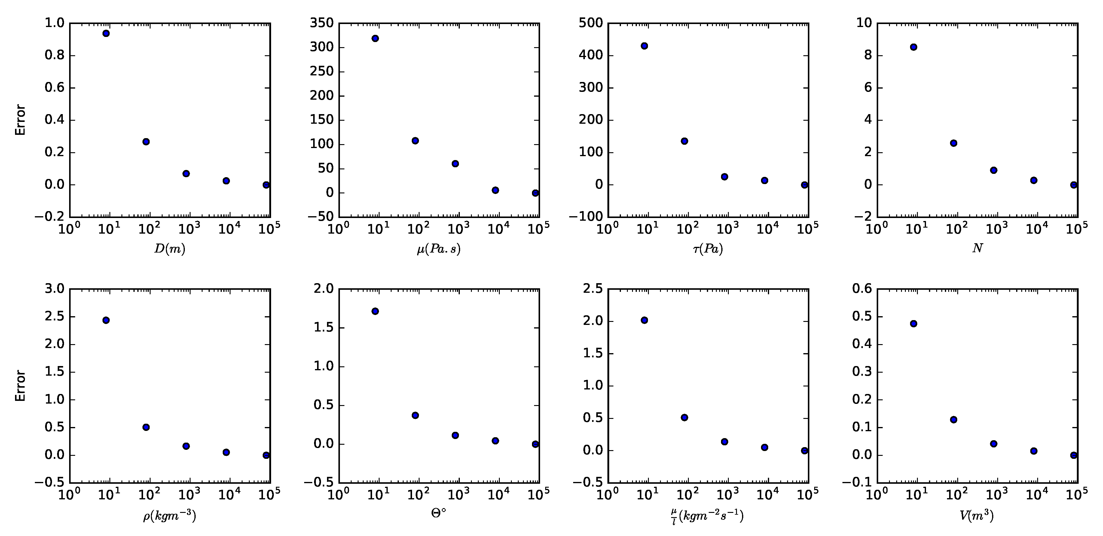
2.4. Variance-Based Sensitivity Analysis

A global sensitivity analysis relies on a number of points scattered evenly through the input parameter space. If a simulator is deterministic, the variance of the output variable is solely the result of uncertainty in the input variables [12]. In an ideal world, the exact values of the input parameters would all be measurable, and the variance of Y (the output) could be reduced to zero. This is not possible here, so we decompose the variance in the output according to the input parameters.

Dakota possesses a variance-based decomposition function which calculates Sobol’ indices [10,31]. The derivation for the Sobol’ indices is as follows. If we fix one parameter $X_i$ at a given value ($x_i$) and rerun the simulator, Y will have a lower overall variance. Suppose the variance is taken over all ranges of input parameters while excepting $X_i$, which is kept fixed. This conditional variance shows how influential the variable $X_i$ is on the variance of Y. However, this method of variance calculation could be strongly affected by the location of the point $x_i$. We can resolve this by taking the average of all these conditional variances over all values of $x_i$ [12]. That is:

$${\mathbb{E}}_i\left[{\mathbb{V}}_{\sim i}\left[Y\right|X_i]\right].$$

(2)

Then we have an expectation of the variance of Y given $X_i$ is fixed, or, put another way, the variance of Y minus the contribution of variance from $X_i$. From probability theory, the variance of a random variable such as Y can be decomposed as follows [12]:

$$\mathbb{V}\left[Y\right]={\mathbb{E}}_i\left[{\mathbb{V}}_{\sim i}\left[Y\right|X_i]\right]+{\mathbb{V}}_i\left[{\mathbb{E}}_{\sim i}\left[Y\right|X_i]\right].$$

(3)

This gives us ${\mathbb{V}}_i\left[{\mathbb{E}}_{\sim i}\left[Y\right|X_i]\right]$, which is the first order effect of $X_i$ on Y. Another way to see this is that if we subtract the expectation of the variance of Y given $X_i$ is fixed from the total variance of Y, we are left with the contribution from $X_i$ only. In this way we can see how influential the input $X_i$ is on the variance in our output Y. We can then normalise this contribution using the total variance of Y. This normalised sensitivity measure is known as a main Sobol’ index [31]:

$$S_i=\frac{{\mathbb{V}}_i\left[{\mathbb{E}}_{\sim i}\left[Y\right|X_i]\right]}{\mathbb{V}\left[Y\right]}.$$

(4)

A high Sobol’ index means that if that input parameter is fixed there will be a significant reduction in the variance of Y. In hazard analysis terms, if we can estimate this kind of input parameter to a high degree of accuracy, then there will be less spread between the predicted best and worst case scenarios.

Many models are non-additive, which means that the effects individual input parameters have on the variance of the output cannot be separated because interactions between individual inputs or sets of inputs play an important role. Therefore, we construct higher order Sobol’ indices [12]:

$$S_p=\frac{{\mathbb{V}}_p\left[{\mathbb{E}}_{\sim p}\left[Y\right|X_i]\right]}{\mathbb{V}\left[Y\right]}.$$

(5)

where $p\subset \{1,\dots ,d\}$ is a subset of indices corresponding to all the inputs that contribute to uncertainty in the output. Full analysis of the effects of all model inputs and their respective interactions will result in the sum of Sobol’ indices having $2^d-1$ terms, which becomes computationally unmanageable quickly. Homma and Saltelli [32] introduced the Total Sobol’ index to summarise these effects:

$$S^{T_i}=1-\frac{{\mathbb{V}}_{{\mathit{X}}_{\sim i}}\left[{\mathbb{E}}_{{\mathit{X}}_i}\left[Y\right|{\mathit{X}}_{\sim i}]\right]}{\mathbb{V}\left[Y\right]},$$

(6)

where ${\mathbb{V}}_{{\mathit{X}}_{\sim i}}$ denotes the conditional variance taken over all variables except ${\mathit{X}}_i$. This captures the variance contribution of the i-th input parameter and all its interactions. In a perfectly additive model, $S_i=S^{T_i}$. It has been argued that a good characterization of the input influences is given by the set of first order and total Sobol’ indices [12].

As described previously, we took the 100 emulators, from a set of 1000 options, with the lowest RMS error between the truth model output and the emulated output. This subset of 100 emulators was selected to confirm how consistent the results of the sensitivity analysis were across different emulator builds. We rebuilt the 100 emulators in this subset using all 120 truth samples in the training data set, but fixing the correlation lengths, which control how rapidly the GPE spreads from the training points, as those optimised by Dakota to the original selection of 80 points. In this way the emulators were validated by the RMS process, but could be trained using all the available training data. We sampled the retrained emulators to perform the variance-based decomposition and obtained main and total Sobol’ indices. For each emulator, we took Latin hypercube samples, using Dakota’s sampling functionality of 8, 80, 800, 8000, and 80,000 points in the parameter space, as a convergence test for the Sobol’ index results.

2.5. Alternative Output Metrics

In order to test the robustness of the variance-based decomposition conclusions, the above method was repeated for two alternative metrics to represent the hazard potential of the LGW. The chosen alternative metrics were the positive displaced volume of water in the wave and an approximation for the run-up of the LGW on an opposite shore.

2.5.1. Volume

The displaced positive volume was chosen as a metric for the hazardousness of the LGW because this value is used as an estimate for inundation volume in tsunami studies [33]. We calculated the maximum volume of water displaced in the positive direction during the simulation for each wave in the training dataset. Then we repeated the emulator construction and variance-based decomposition approaches described in Section 2.3 and Section 2.4.

2.5.2. Run-Up

The run-up was chosen as another output metric to incorporate some investigation of the interaction of the LGW with an opposite shore into our analysis. Run-up is complex to directly simulate; hence, we estimated the run-up based on the analytical relation [34]:

$$R=2.831H_0{\left(\frac{H_0}{d}\right)}^{\frac{1}{4}}\sqrt{cot\beta },$$

(7)

where $H_0$ is the maximum wave height in the open ocean, d is the open ocean water depth, and $\beta$ is the slope angle of the beach. We assumed the wave generated in our SPH simulations propagated in the same direction as the slide motion until it reached a shore where the run-up could be estimated. We used the values of maximum wave height extracted from our SPH simulations as the values of $H_0$. This approximation for run-up is not dependent on the distance the wave propagates. Calculating run-up by Equation (7), therefore, introduced just two additional input parameters to our sensitivity analysis: the open ocean water depth, d, and the beach slope angle, $\beta$ (shown in Figure 1). These variables were also sampled 120 times using a Sobol’ sequence so that they could be included in the emulation and VBD process. The bounds for d were chosen as 100 m and 500 m, and the bounds for $\beta$ were set as ${0.5}^{\circ }$ and ${8.0}^{\circ }$, in keeping with our Alaskan bay scale scenario. Once values for R had been calculated for each of the 120 sets of ten input parameters, 1000 emulators were built and tested. The 100 that performed best were used for the VBD analysis.

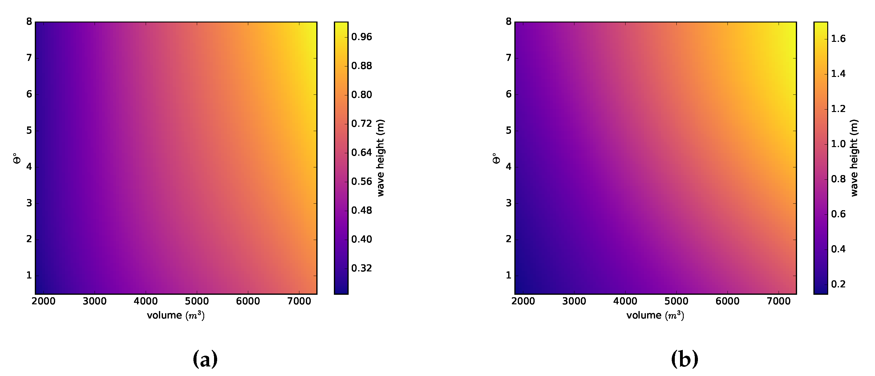
2.6. Analysis of Parameter Interactions

As mentioned in Section 2.4, a variance-based decomposition can calculate both main and total Sobol’ indices (Equations (4) and (6)). The total Sobol’ indices provide insight into interaction between parameters, which could potentially augment the output or complicate its prediction. We therefore investigated some of these parameter interactions.

The total Sobol’ indices do not indicate which parameters interact with each other, but simply the amount each parameter contributes to the total variance through interactions. We took the parameters that showed the highest interactions and compared them pairwise using the emulator and Dakota’s Latin hypercube sampling routine. For each comparison, all other parameters were kept constant at their mean values by default. The purpose of this analysis was to seek regimes in which parameters showed interesting interactions and where those interactions have important implications for larger scale LGWs.

3. Results

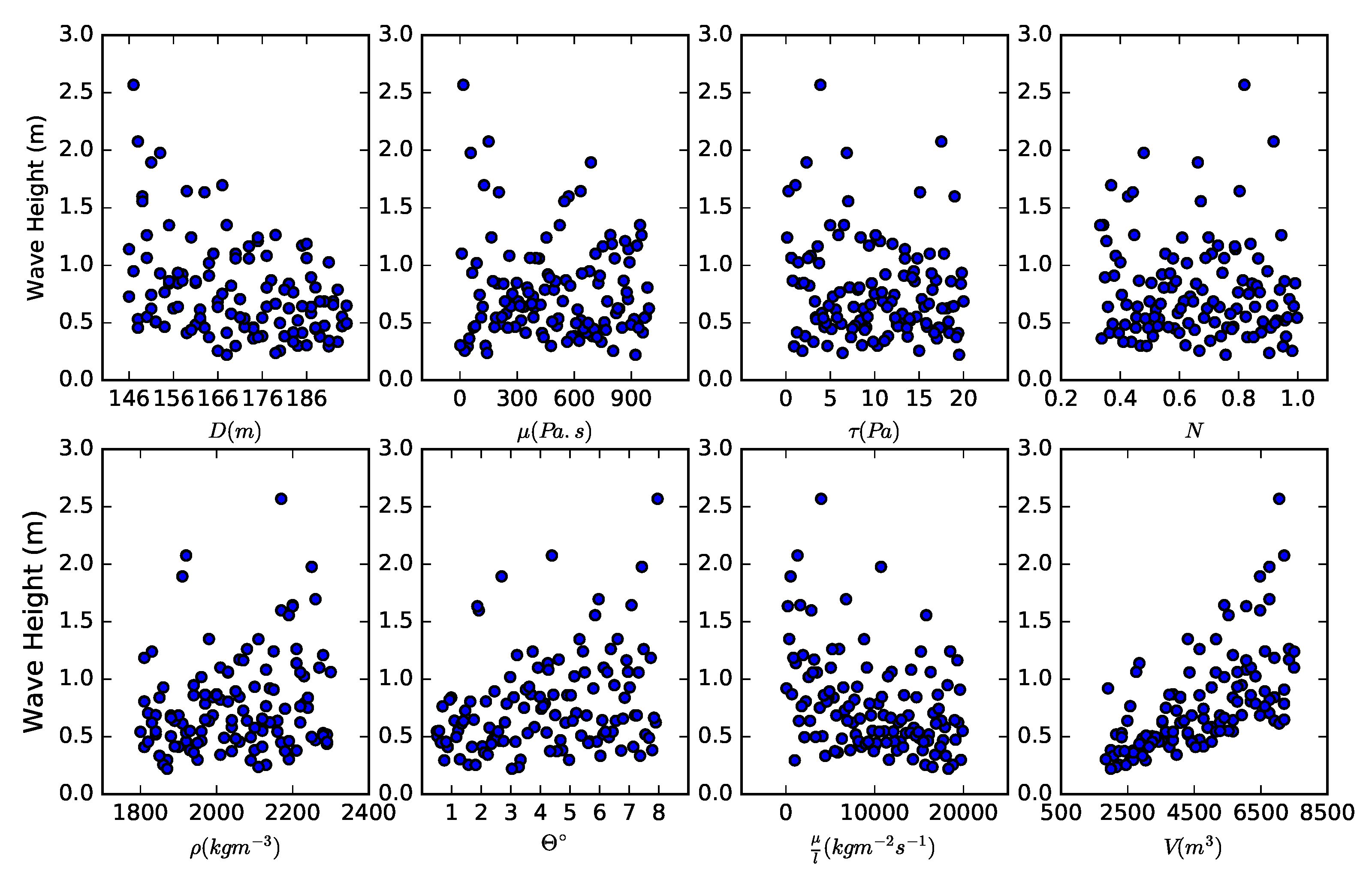
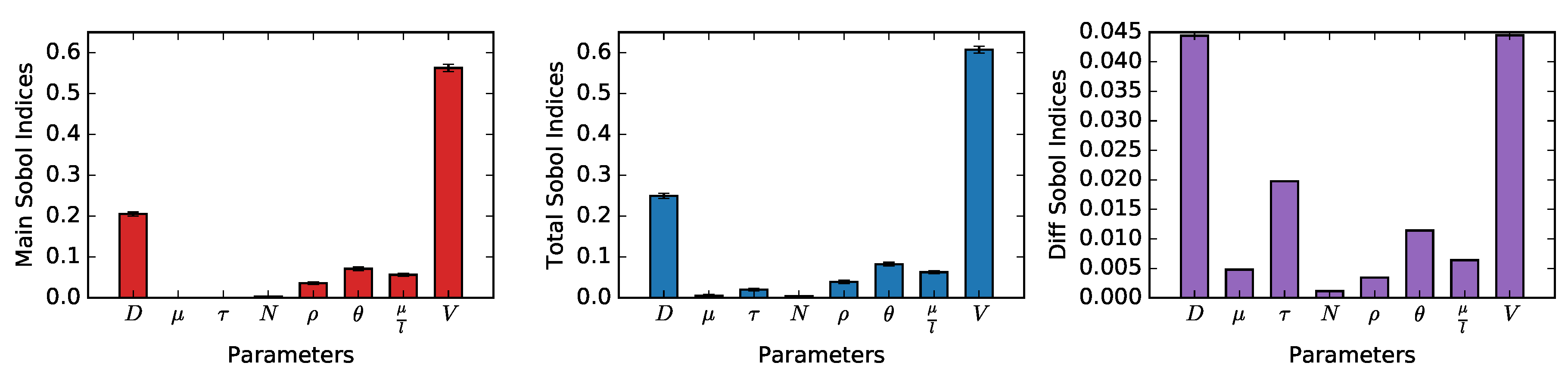
3.1. Wave Height Results

The results of the training data from the truth (SPH) model are shown in Figure 4 as scatter plots between each input parameter and the value of the maximum surface elevation for that truth run. If one input parameter had far and away the greatest influence on the variance of the output, a trend would be clear in one of these panels. As Figure 4 shows, the landslide volume has a strong influence, because a positive trend emerges between it and the wave height. The variance-based decomposition and calculation of Sobol’ indices quantify trends like this.

The results of the VBD convergence test are shown in Figure 5. These results show the mean error at each sample size, taken over the 100 emulators that had the lowest RMS errors between the 40 truth and emulated test values. Satisfactory convergence towards zero error was achieved for the values of the Sobol’ indices for all input parameters by taking 8000 emulator samples. Volume, depth, and slope angle showed fairly rapid convergence, while the rheological parameters ($\mu$, $\tau$, and N) showed the slowest convergence.

The mean values of the main and total Sobol’ indices, calculated from the 100 emulators with the lowest RMS values, are shown in Figure 6. Shown also are the differences between the main and total indices, which demonstrate which input parameters strongly interact.

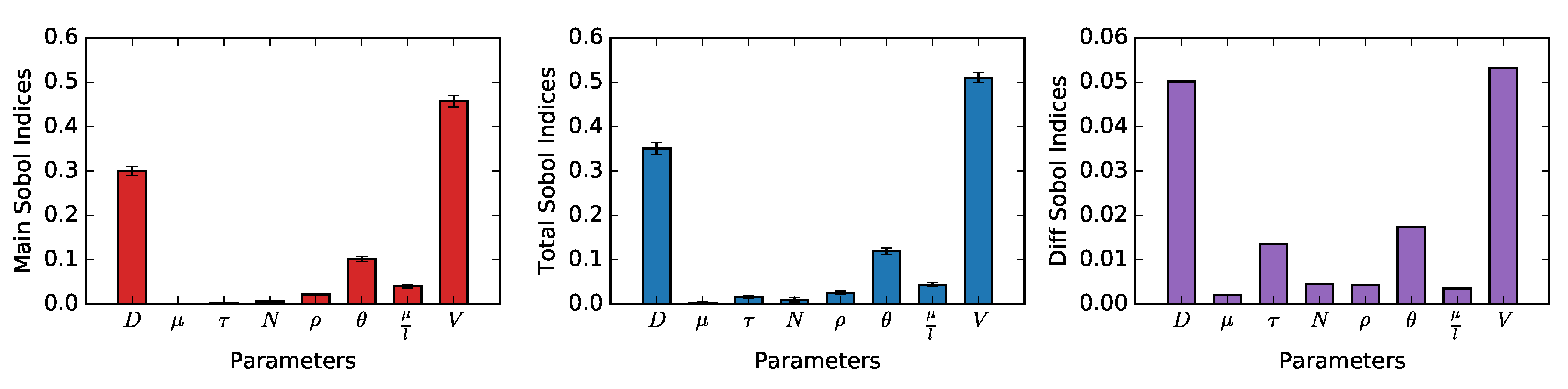
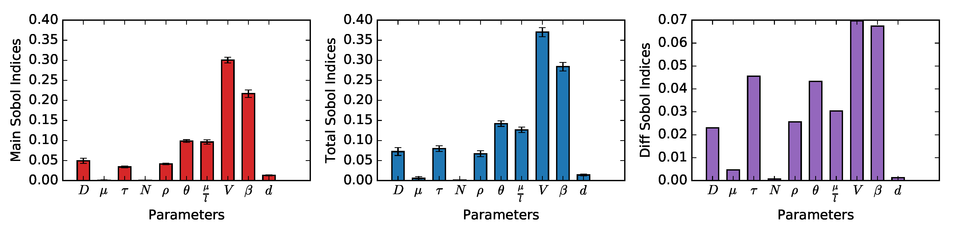
3.2. Alternative Output Metric Results

We repeated the GPE and VBD method for the two additional output metrics: positive displaced water volume and approximated run-up. The average Sobol’ indices calculated from 100 of the best performing emulators in each case are shown in Figure 7 and Figure 8. In addition to the 8 original input parameters, the VBD using run-up as a metric includes the maximum water depth offshore (d) and the slope angle of the inundated shore ($\beta$).

3.3. Parameter Interactions

For maximum wave height, the parameters which show the highest levels of interaction are V and D, followed by $\tau$ and $\theta$. A three way comparison between V, $\theta$, and $\tau$, revealed the results shown in Figure 9.

When the slide has high yield stress, the effect of volume dominates over slope angle in terms of maximum wave height. This means that small volume slides do not produce large waves at any slope angle. However, as yield stress decreases, this unlocks the potential for small volume slides to produce waves at high slope angles (Figure 9b).

Interaction between $\tau$ and $\frac{\mu }{l}$ was also revealed by our analysis. Figure 10 shows the wave heights predicted by the emulator for values of $\tau$ and $\frac{\mu }{l}$ throughout their parameter space, with all other input parameters set at their mean values. Low values of $\tau$ and $\frac{\mu }{l}$ would be expected to produce large waves. We do see this, but fairly large waves are also produced at all values of $\tau$ for low $\frac{\mu }{l}$ and at all values of $\frac{\mu }{l}$ for low $\tau$. In other words, only one of these parameters needs to be small to produce larger waves. This effect propagated through to the inundation stage.

3.4. Discussion

For the maximum wave height output metric the parameters that contribute the most to the variance of the output are the landslide volume, V, and the initial submergence depth, D. The bottom boundary condition, $\frac{\mu }{l}$, and slope angle, $\theta$, show moderate contributions to variance. The high contributions of volume and landslide submergence depth to variance in the simulated wave height (Figure 4) match findings by other studies [5,6,35]. The importance of slope angle and bottom boundary condition follow from the strong effects these parameters have on the initial acceleration of the landslide.

Interestingly, the yield stress, which might be expected to have a significant effect on initial acceleration, is not seen to have a very high main Sobol’ index. This may be because the boundary condition parameter that simulates the interaction between the base of the slide and the slope spans the full range between no-slip to full-slip. Hence, the contribution of the boundary condition parameter to variance in the output swamps the contributions of yield stress, viscosity, and shear thinning. This observation indicates that we could model landslides with fewer rheological input parameters and simply use the bottom boundary condition as a controlling parameter. However, this boundary condition does not currently have precise physical constraints. It does span the full range of numerical modelling choices, i.e., no-slip to full-slip, but as yet there is no way to constrain the value that it should take in a given scenario. Deriving the appropriate boundary condition parameter via validation experiments or from full-scale scenario analysis would be grounds for further study.

The Sobol’ indices for the positive displaced volume metric show the same ordering of input parameters as they do for wave height, with V and D contributing the most to variance. For this output metric the three secondary parameters ($\theta$, $\frac{mu}{l}$, $\rho$) show greater differences in their main Sobol’ indices than they do for the wave height, with the slope angle contributing more to variance than the other two. The similarity between the Sobol’ indices for wave height and positive displaced volume is encouraging, because it implies these represent two equivalent ways to assess the hazard posed by a LGW.

Wave run-up, calculated using the analytical relation (7), adds two additional input parameters that contribute to uncertainty. Our results (Figure 8) show that if run-up is used to diagnose the hazard of an LGW, landslide volume is still the most influential parameter. The slope angle of the inundated shore ($\beta$) is the second largest contributor to variance in the run-up. This implies that characterisation of the target location is nearly as important as the source characterisation when assessing hazard. Further investigation of the parameters that contribute to uncertainty in the run-up would therefore be beneficial. For example, rather than using a run-up approximation, a hydrodynamic model capable of capturing wave propagation, shoaling, and frictional effects during inundation would likely provide more insights.

The parameter interactions we presented provide some interesting insight as to the effect of rheology, specifically yield stress ($\tau$), on the simulated wave characteristics. Although the main Sobol’ index of $\tau$ for each of the output metrics was small, its interactions in all three cases were substantial. We first performed a three-way comparison of volume, slope angle, and yield stress. This showed that as yield stress decreased it unlocked the potential of small volume landslides to cause waves at steep slope angles. This is significant for hazard analysis because it is difficult to directly measure the yield stress of a landslide, and therefore hard to include it in a predictive hazard model. Understanding a parameter interaction like this allows for more complete understanding of the potential hazard posed by a small volume landslide, for example, if it had a low yield stress.

The second parameter interaction we presented was between yield stress and the bottom boundary condition. Our findings here are significant from a modelling perspective, because the interaction showed that only one of these parameters had to be small for large waves to be generated by a landslide. In other words, if either parameter is small, a lubricating bottom boundary layer will exist and the landslide will accelerate faster. From a modelling perspective, this interaction implies that using just one of these parameters should be sufficient to capture the essential physics, with a boundary layer either being implicitly modelled by the bottom boundary condition or explicitly resulting from the slide behaviour near the wall. However, both were included in this study because a physical constraint for the bottom boundary condition is not available as yet, and observations suggest that landslides exhibit yield stress even if the value of it is hard to determine. Although yield stress interacted with other parameters strongly, the bottom boundary condition had a higher main Sobol’ index. This suggests a future study on better simulating the interaction between slide and slope would be worthwhile.

4. Conclusions

Here we developed a Gaussian process emulator (GPE) of a Smooth Particle Hydrodynamics (SPH) simulator to assess uncertainty in landslide generated waves (LGWs). The SPH simulator enabled a detailed exploration of the source parameters that contribute to uncertainty in simulated LGWs, because it was capable of modelling complex slide rheologies and a variable boundary condition between the base of the slide and the underlying slope. We used a dataset of SPH simulations that efficiently represented the input parameter space to train GPEs. These GPEs were then used to perform a variance-based sensitivity analysis. We considered three separate output metrics to assess the hazard posed by a given landslide scenario: the maximum wave height, maximum positive displaced volume of the wave, and approximated run-up.

The variance-based sensitivity analysis revealed the input parameters to our SPH simulator that were responsible for the most variance in the three output metrics. In the case of maximum wave height and displaced volume, the volume of the landslide and the landslide submergence depth contribute the most to the variance, closely followed by the slope angle and the viscosity of the boundary layer. Current understanding of LGWs indicates landslide volume, submergence depth and initial acceleration are the major controls on LGW hazard [4,5,6]. Our findings corroborate this, as the slope angle and bottom boundary layer viscosity have a direct effect on the initial acceleration of the landslide. When wave run-up at the shore was used as the output metric, the slope angle of the shore was a highly influential parameter, second after landslide volume. This implies that characteristics of the target area of interest in a hazard analysis should be included along with source characteristics, and both should be treated jointly in an uncertainty analysis.

Critically, the methodology shown here demonstrates promise for probabilistic hazard analyses that rely on computationally costly truth models. By establishing the rankings of the contributions of the input parameters to variance in the output metric, future effort and computational resources can focus on reducing the uncertainty surrounding input parameters that make larger contributions. Similarly, input parameters that consistently contribute very little to variance in the output could be discounted from future analyses.

Our study reveals several areas for future work. Firstly, attempting to constrain the boundary layer viscosity physically would reduce uncertainty in output predictions and may also preclude the need for the use of complex rheological models. Secondly, considering parameters that characterise the propagation and inundation phases of the LGW life cycle, such as propagation distance and the slope angle of the inundated shore, would be advisable. The use of a run-up approximation revealed that the slope of the shore was an important parameter, but there are many parameters and processes that this run-up approximation does not cover. Such processes may include highly nonlinear 3D and dispersive effects during propagation, wave shoaling, and friction as the wave travels over land. A study employing hydrodynamic models capable of capturing processes like these and employing a similar uncertainty quantification method would be valuable. Finally, extending this analysis to include 3D LGW models could reveal some as-yet-unexplored influences of input parameters or parameter interactions on the simulated LGW.

References

1. Bugge, T.; Belderson, R.; Kenyon, N. The Storegga slide. Philos. Trans. R. Soc. Ser. A 1988, 325, 358–390. [Google Scholar]
2. Piper, D.J.W.; Cochonat, P.; Morrison, M.L. The sequence of events around the epicentre of the 1929 Grand Banks earthquake: Initiation of the debris flows and turbidity current inferred from side scan sonar. Sedimentology 1999, 46, 79–97. [Google Scholar] [CrossRef]
3. Harbitz, C.; Løvholt, F.; Bungum, H. Submarine landslide tsunamis: How extreme and how likely? Nat. Hazards 2014, 72, 1341–1374. [Google Scholar] [CrossRef]
4. Yavari-Ramshe, S.; Ataie-Ashtiani, B. Numerical modeling of subaerial and submarine landslide-generated tsunami waves—Recent advances and future challenges. Landslides 2016, 1–44. [Google Scholar] [CrossRef]
5. Ataie-Ashtiani, B.; Najafi-Jilani, A. Laboratory investigations on impulsive waves caused by underwater landslide. Coast. Eng. 2008, 55, 989–1004. [Google Scholar] [CrossRef]
6. Grilli, S.; Shelby, M.; Kimmoun, O.; Dupont, G.; Nicolsky, D.; Ma, G.; Kirby, J.; Shi, F. Modeling coastal tsunami hazard from submarine mass failures: Effects of slide rheology, experimental validation, and case studies off the US East Coast. Nat. Hazards 2016, 86, 353–391. [Google Scholar] [CrossRef]
7. Wagener, T.; Pianosi, F. What has Global Sensitivity Analysis ever done for us? A systematic review to support scientific advancement and to inform policy-making in earth system modelling. Earth-Sci. Rev. 2019, 194, 1–18. [Google Scholar] [CrossRef]
8. Monaghan, J. Smoothed Particle Hydrodynamics and Its Diverse Applications. Annu. Rev. Fluid Mech. 2012, 44, 323–346. [Google Scholar] [CrossRef]
9. Neethling, S.J.; Barker, D.J. Using Smooth Particle Hydrodynamics (SPH) to model multiphase mineral processing systems. Miner. Eng. 2016, 90, 17–28. [Google Scholar] [CrossRef]
10. Sandia National Laboratories. Dakota, a Multilevel Parallel Object-Oriented Framework for Design Optimization, Parameter Estimation, Uncertainty Quantification, and Sensitivity Analysis: Version 6.5 User Manual; Sandia National Laboratories: Albuquerque, NM, USA, 2016.
11. Salmanidou, D.; Guillas, S.; Georgiopoulou, A.; Dias, F. Statistical emulation of landslide-induced tsunamis at the Rockall Bank, NE Atlantic. Proc. R. Soc. A Math. Phys. Eng. Sci. 2017, 473. [Google Scholar] [CrossRef] [Green Version]
12. Hristov, P.; DiazDelaO, F.; Saavedra Flores, E.; Guzmán, C.; Farooq, U. Probabilistic sensitivity analysis to understand the influence of micromechanical properties of wood on its macroscopic response. Compos. Struct. 2017, 181, 229–239. [Google Scholar] [CrossRef] [Green Version]
13. Murphy, J.; Sexton, D.; Jenkins, G.; Boorman, P.; Booth, B.; Brown, C.; Clark, R.; Collins, M.; Harris, G.; Kendon, E.; et al. UK Climate Projections Science Report: Climate Change Projections; Met Office Hadley Centre: Exeter, UK, 2009.
14. Schambach, L.; Grilli, S.T.; Kirby, J.; Shi, F. Landslide Tsunami Hazard Along the Upper US East Coast: Effects of Slide Deformation, Bottom Friction, and Frequency Dispersion. Pure Appl. Geophys. 2018. [Google Scholar] [CrossRef]
15. Snelling, B.; Collins, G.; Piggott, M.; Neethling, S. Improvements to a Smooth Particle Hydrodynamics simulator for investigating submarine landslide generated waves. Int. J. Numer. Methods Fluids. in review. [CrossRef]
16. Monaghan, J.; Kos, A.; Issa, N. Fluid Motion Generated by Impact. J. Waterw. Port Coast. Ocean Eng. 2003, 129, 250–259. [Google Scholar] [CrossRef]
17. Ataie-Ashtiani, B.; Shobeyri, G. Numerical Simulation of Landslide Impulsive Waves by Incompressible Smoothed Particle Hydrodynamics. Int. J. Numer. Methods Fluids 2008, 56, 209–232. [Google Scholar] [CrossRef]
18. Capone, T.; Panizzo, A.; Monaghan, J.J. SPH modelling of water waves generated by submarine landslides. J. Hydraul. Res. 2010, 48, 80–84. [Google Scholar] [CrossRef]
19. Heller, V.; Bruggemann, M.; Spinneken, J.; Rogers, B. Composite modelling of subaerial landslide-tsunamis in different water body geometries and novel insight into slide and wave kinematics. Coast. Eng. 2016, 109, 20–41. [Google Scholar] [CrossRef]
20. Laigle, D.; Coussot, P. Numerical Modeling of Mudflows. J. Hydraul. Eng. 1997, 123, 617–623. [Google Scholar] [CrossRef]
21. Sawyer, D.; Flemings, P.; Buttles, J.; Mohrig, D. Mudflow transport behavior and deposit morphology: Role of shear stress to yield strength ratio in subaqueous experiments. Mar. Geol. 2012, 307–310, 28–39. [Google Scholar] [CrossRef]
22. Nicolsky, D.J.; Suleimani, E.N.; Haeussler, P.J.; Ryan, H.F.; Koehler, R.D.; Combellick, R.A.; Hansen, R.A. Tsunami Inundation Maps of Port Valdez, Alaska; Alaska Division of Geological Geophysical Surveys: Fairbanks, AK, USA, 2013. [CrossRef] [Green Version]
23. Suleimani, E.; Hansen, R.; Haeussler, P. Numerical study of tsunami generated by multiple submarine slope failures in Resurrection Bay, Alaska, during the MW 9.2 1964 earthquake. Pure Appl. Geophys. 2009, 166, 131–152. [Google Scholar] [CrossRef]
24. Harbitz, C. Model simulations of tsunamis generated by the Storegga Slides. Mar. Geol. 1992, 105, 1–21. [Google Scholar] [CrossRef]
25. Iverson, R. The physics of debris flows. Rev. Geophys. 1997, 35, 245–296. [Google Scholar] [CrossRef] [Green Version]
26. Coussot, P.C. Mudflow Rheology and Dynamics: IAHR-AIRH Monographs; AA Balkema Publishers: Rotterdam, The Netherlands, 1997. [Google Scholar]
27. Blasio, F.D.; Elverhøi, A.; Issler, D.; Harbitz, C.; Bryn, P.; Lien, R. On the dynamics of subaqueous clay rich gravity mass flows—The giant Storegga slide, Norway. Mar. Pet. Geol. 2005, 22, 179–186. [Google Scholar] [CrossRef]
28. Abadie, S.; Morichon, D.; Grilli, S.; Glockner, S. Numerical simulation of waves generated by landslides using a multiple-fluid Navier–Stokes model. Coast. Eng. 2010, 57, 779–794. [Google Scholar] [CrossRef]
29. De Blasio, F.V. Introduction to the Physics of Landslides: Lecture Notes on the Dynamics of Mass Wasting; Springer: Berlin, Germany, 2011. [Google Scholar]
30. Sobol’, I. On the distribution of points in a cube and the approximate evaluation of integrals. USSR Comput. Math. Math. Phys. 1967, 7, 86–112. [Google Scholar] [CrossRef]
31. Sobol’, I. Global sensitivity indices for nonlinear mathematical models and their Monte Carlo estimates. Math. Comput. Simul. 2001, 55, 271–280. [Google Scholar] [CrossRef]
32. Homma, T.; Saltelli, A. Importance measures in global sensitivity analysis of nonlinear models. Reliab. Eng. Syst. Saf. 1996, 52, 1–17. [Google Scholar] [CrossRef]
33. Bryant, E. Tsunami: The Underrated Hazard; Springer: Berlin, Germany, 2014; pp. 1–222. [Google Scholar]
34. Synolakis, C. The runup of solitary waves. J. Fluid Mech. 1987, 185, 523–545. [Google Scholar] [CrossRef]
35. Harbitz, C.; Løvholt, F.; Pedersen, G.; Masson, D. Mechanisms of tsunami generation by submarine landslides: A short review. Nor. Geol. Tidsskr. 2006, 86, 255–264, cited By 130. [Google Scholar]
Figure 1. Geometry for training dataset. The variables D, θ , d, and β shown in the sketch are described in Table 1. The distance from the left hand side of the Smooth Particle Hydrodynamics (SPH) domain to the mid-point of the slide averages 582 m is shown, but varies slightly with the slope angle θ . The SPH simulation domain is shown along with a sketch of the idealised geometry assumed for our run-up approximation (Section 2.5.2).
Water 12 00416 g001
Figure 2. Test case for the range of boundary layer viscosities. The two extreme values coincide well with the no- and full-slip cases.
Water 12 00416 g002
Figure 3. Wave heights calculated from the truth model (SPH) compared to emulated wave heights from the GPE, for the same 40 sets of input parameters. Red line shows the 1:1 trend.
Water 12 00416 g003
Figure 4. Scatter of simulated wave heights from all the truth model runs against each of the input parameters. Plots where the input parameter has a strong influence on the simulated wave height should show a trend, despite the variation in all the other input parameters across different truth runs.
Water 12 00416 g004
Figure 5. Convergence of values of main Sobol’ indices with increasing samples of the emulator (8, 80, 800, 8000, 80,000). Reasonable convergence was achieved for indices corresponding to each parameter input by 8000 samples.
Water 12 00416 g005
Figure 6. Mean values of the main and total Sobol’ indices obtained by 80,000 LHS samples of the 100 emulators with lowest RMS errors. Shown also are the differences between the main and total Sobol’ indices for each input parameter. Error bars show standard deviations about the mean. The input parameters, as shown along the x axis, are: submergence depth, D ( m ) ; viscosity, μ ( P a   s ) ; yield stress, τ ( P a ) ; shear thinning exponent, N; density, ρ ( k g   m 3 ) ; slope angle, θ ; boundary layer parameter, μ l ( k g   m 2   s 1 ) ; and volume, V ( m 3 ) .
Water 12 00416 g006
Figure 7. Sobol’ indices calculated from positive displaced volume of waves. The input parameters, as shown along the x axis, are: submergence depth, D ( m ) ; viscosity, μ ( P a   s ) ; yield stress, τ ( P a ) ; shear thinning exponent, N; density, ρ ( k g   m 3 ) ; slope angle, θ ; boundary layer parameter, μ l ( k g   m 2   s 1 ) ; and volume, V ( m 3 ) .
Water 12 00416 g007
Figure 8. Sobol’ indices calculated from run-up, approximated using Equation (7). The input parameters as shown along the x axis are: submergence depth, D ( m ) ; viscosity, μ ( P a   s ) ; yield stress, τ ( P a ) ; shear thinning exponent, N; density, ρ ( k g   m 3 ) ; slope angle, θ , boundary layer parameter; μ l ( k g   m 2   s 1 ) ; volume, V ( m 3 ) ; inundated slope angle, β ; and maximum offshore water depth, d ( m ) .
Water 12 00416 g008
Figure 9. Volume, slope angle, and yield stress three way comparison. Yield stress is decreasing from left to right. Volume and slope angle were sampled throughout their ranges, and all other parameters were fixed at their mean values. (a) Maximum wave height predicted by the emulator for given volume and slope angle and maximum yield stress. (b) Maximum wave height predicted by the emulator for given volume and slope angle and minimum yield stress.
Water 12 00416 g009
Figure 10. Wave height comparison for yield stress and boundary layer viscosity, with all other parameters at mean values.
Water 12 00416 g010