Discussion

Mesoscale Mapping of Sediment Source Hotspots for Dam Sediment Management in Data-Sparse Semi-Arid Catchments

1
Research Group Ecohydrology and Landscape Evaluation, Technical University Berlin, 10587 Berlin, Germany
2
Institute of Environmental Science and Geography, University of Potsdam, 14467 Potsdam, Germany
3
Avaye Ab Shabnam Consulting Engineering Company, 6133883441 Ahvaz, Iran
4
Dam Complex of Upper Atbara, 11605 Khartoum, Sudan
5
Khuzestan Water and Power Authority, 61355-137 Ahvaz, Iran
6
Iran Water Resources Management Co., 14896 Tehran, Iran
*
Author to whom correspondence should be addressed.
Water 2020, 12(2), 396; https://doi.org/10.3390/w12020396
Submission received: 17 December 2019 / Revised: 18 January 2020 / Accepted: 20 January 2020 / Published: 1 February 2020
(This article belongs to the Section Water Resources Management, Policy and Governance)

Abstract

:
Land degradation and water availability in semi-arid regions are interdependent challenges for management that are influenced by climatic and anthropogenic changes. Erosion and high sediment loads in rivers cause reservoir siltation and decrease storage capacity, which pose risk on water security for citizens, agriculture, and industry. In regions where resources for management are limited, identifying spatial-temporal variability of sediment sources is crucial to decrease siltation. Despite widespread availability of rigorous methods, approaches simplifying spatial and temporal variability of erosion are often inappropriately applied to very data sparse semi-arid regions. In this work, we review existing approaches for mapping erosional hotspots, and provide an example of spatial-temporal mapping approach in two case study regions. The barriers limiting data availability and their effects on erosion mapping methods, their validation, and resulting prioritization of leverage management areas are discussed.

1. Introduction

Siltation of reservoirs (also called sediment entrapment or infilling of reservoirs) is a major problem in semi-arid regions where water is scarce and land degradation frequently results in high sediment loads in rivers entering reservoirs [1,2,3,4]. The sediment inflow in reservoirs reduces water storage volume, thereby endangering the water available for citizens, irrigated agriculture, and hydropower energy generation [5]. When water is the dominant mechanism of soil loss across a catchment, soil-water conservation measures in sediment source areas can drastically decrease catchment sediment yields [6,7]. Modeling and monitoring studies showed that timely and spatially adjusted management can significantly decrease downstream sediment delivery [8,9,10]. However, sediment sources are unknown in many semi-arid catchments, and no data are available to adjust management accordingly. Moreover, limited financial resources to apply soil-water conservation measures and institutional barriers pose further challenges for water and land managers [11]. In such situations, identifying and managing areas contributing to high sediment yields (as sediment hotspots) are crucial to decrease sediment inputs to reservoirs. We define “leverage areas” as sediment hotspots where management would have the greatest impact on reducing erosion and sediment delivery into downstream bodies (e.g., dam, catchment and outlet).
Several methods have been developed to define hotspots areas (or areas with high erosion risk) which would particularly benefit from further management. Methods differ mainly in: (i) sub-processes and mechanisms of water erosion being considered [12,13,14]; (ii) factors controlling of water erosion and sediment delivery [15]; (iii) representation of relationships between factors, including representation within conceptual, empirical, statistical, or physics-based models [16,17,18]; and (iv) study areas and scales. Commonalities among these approaches are: (i) difficulties ensuring the same input data quality for whole study area; (ii) ensuring the same spatial and temporal precision and quality of data for each controlling factor; (iii) validation of mapped areas; and (iv) disclosure of the most appropriate decision rules for identifying hotspots and leverage areas [19,20,21,22,23].
Application of sediment hot spot mapping and delivery of reliable outputs is limited by data availability and understanding of the processes driving sediment delivery in respective catchments. The misidentification of sediment sources and pathways increases the risk of reservoir infilling with serious consequences on water shortages in semi-arid regions already unprivileged in many aspects (e.g., economically and environmentally). Retaining reservoir volumes is of primary importance for sustaining drinking water, irrigation water availability, and hydropower generation, and is a primary concern of water managers. This study aimed to illustrate why and how data availability constrains the identification of key leverage areas for sediment management. We investigated mapping approaches for erosion hotspot mapping, and on two examples of data-sparse mesoscale catchments (in Iran and Sudan) illustrated how mapping of sediment of hotspots in data sparse semi-arid catchments can be enhanced using freely available global datasets. Lastly, we discuss which methodological approaches can be applied for mapping spatial and temporal variability and for validating results, and which challenges are common for research and management in data sparse areas.

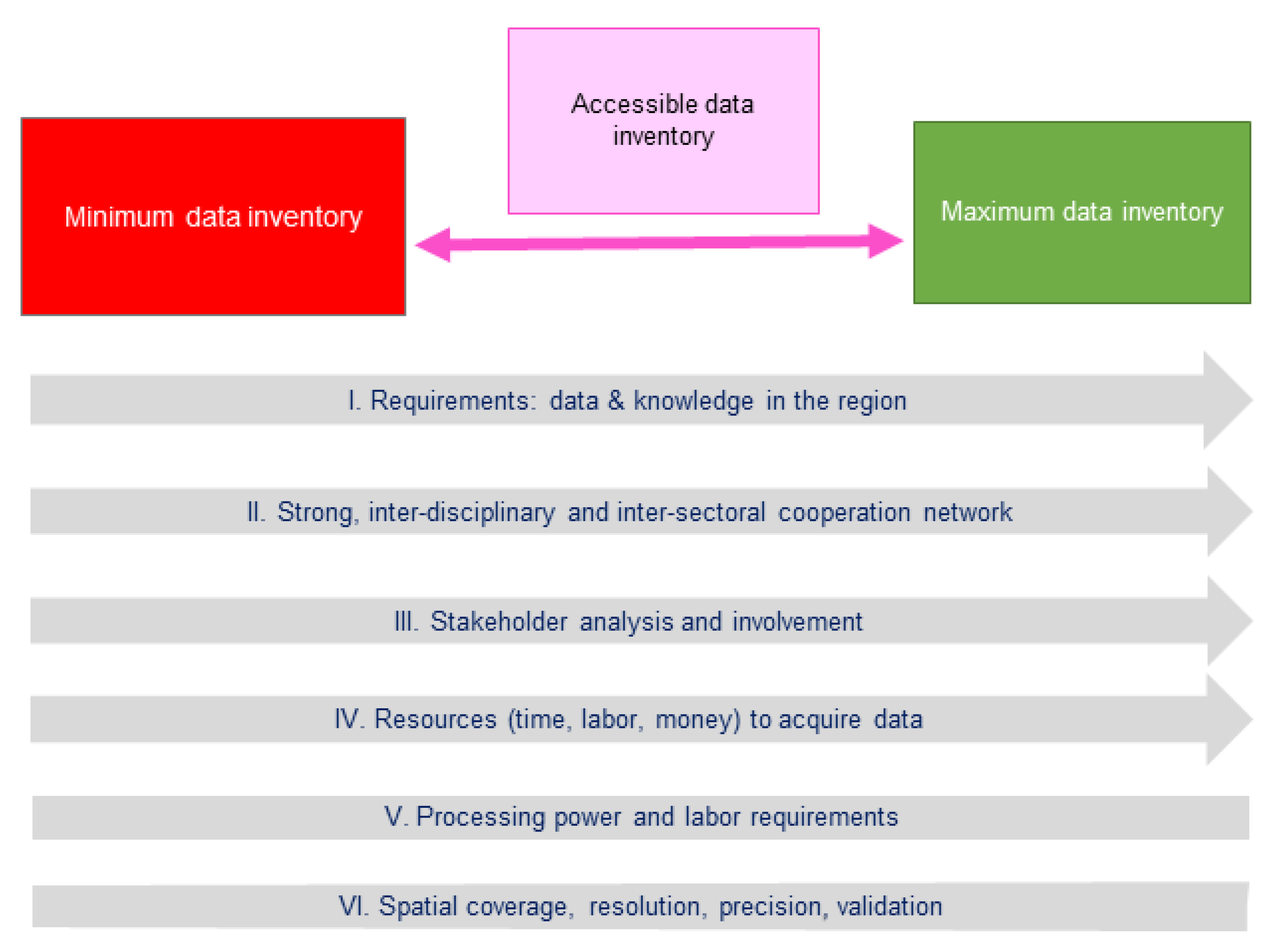
2. Constraints on Data Availability

When it comes to data availability and sharing, researchers across the globe, administrators, mangers of land and water resources, and planners of companies designing new infrastructures (furthermore stakeholders) encounter similar constraints, all rooted in:
  • general data unavailability due to a lack of, a decline in, or unequal distribution of monitoring and measuring stations [24,25];
  • low or questionable quality of existing data due to false research design or poor documentation [26,27,28];
  • inaccessibility of data due to un-/official institutional policies or stakeholders’ personal preferences for cross-institutional data sharing and co-production, including digitalization and use of data [26,28,29].
The above-listed data limitations define an operating space for the preparation of a management plan. The degree to which a management plan can fit the actual natural and socioeconomic processes influencing sediment delivery is directly linked to data available for stakeholders (as well as data inventory), and to the methodological tools they have available and are able to use. In principal, two inventory types—minimum and maximum (Figure 1)—define stakeholders’ operating space. Maximum data inventories are all data collected in a region of interest by various research, administration, and commercial institutions, which might be not available for analysis before or during the entirety of a management-planning project. On the other hand, minimum data inventories are the minimal data needed to identify leverage areas. These data are (or rather principally should be) freely available data (globally and regionally). The accessible data inventory includes the data which the stakeholder use in a specific time period for conducting research or analysis to support management decisions. Accessible data inventory can differ for different stakeholders (institution or person) responsible for the analysis.
Six conditions (requirements or processes) challenge the stakeholder conducting research or analysis to support management decisions: (i) requirement on data and knowledge in the region of interest; (ii) inter-disciplinary and inter-sectoral cooperation network; (iii) stakeholder analysis and involvement; (iv) resources (time, labor, money) to acquire data; (v) processing power and labor requirements; and (vi) spatial coverage, resolution, precision, validation. Conditions I–IV (in Figure 1) are related to internal and external institutional environments, and Conditions V and VI are more data related. They have various degree of complexity (increase in complexity is indicated by arrows in Figure 1). The complexity of data related challenges is not indicated, while it differs between types of datasets. For example, complexity can increase in sediment yield evaluation using multiple methods and maximum inventory in a catchment. In this scenario, researchers may have rainfall simulations, hillslope and runoff plot monitoring, lysimeters and gully head retreat measurements, sediment fingerprinting, legacy sediment analysis, and river discharge and sediment monitoring at their disposal. Alternatively, remote sensing-based monitoring of regional vegetation growth using minimum inventory provides better spatial information coverage in comparison to vegetation mapping, which is usually not performed at large scales or continuously due to enormous labor requirements. In this scenario, processing of remote-sensing based monitoring requires high processing power, sophisticated algorithms, and well-trained users.
Data inventories can limit or enhance sediment hotspot mapping and delivery. Subsequently, we review mapping approaches developed under constraints of unavailability.

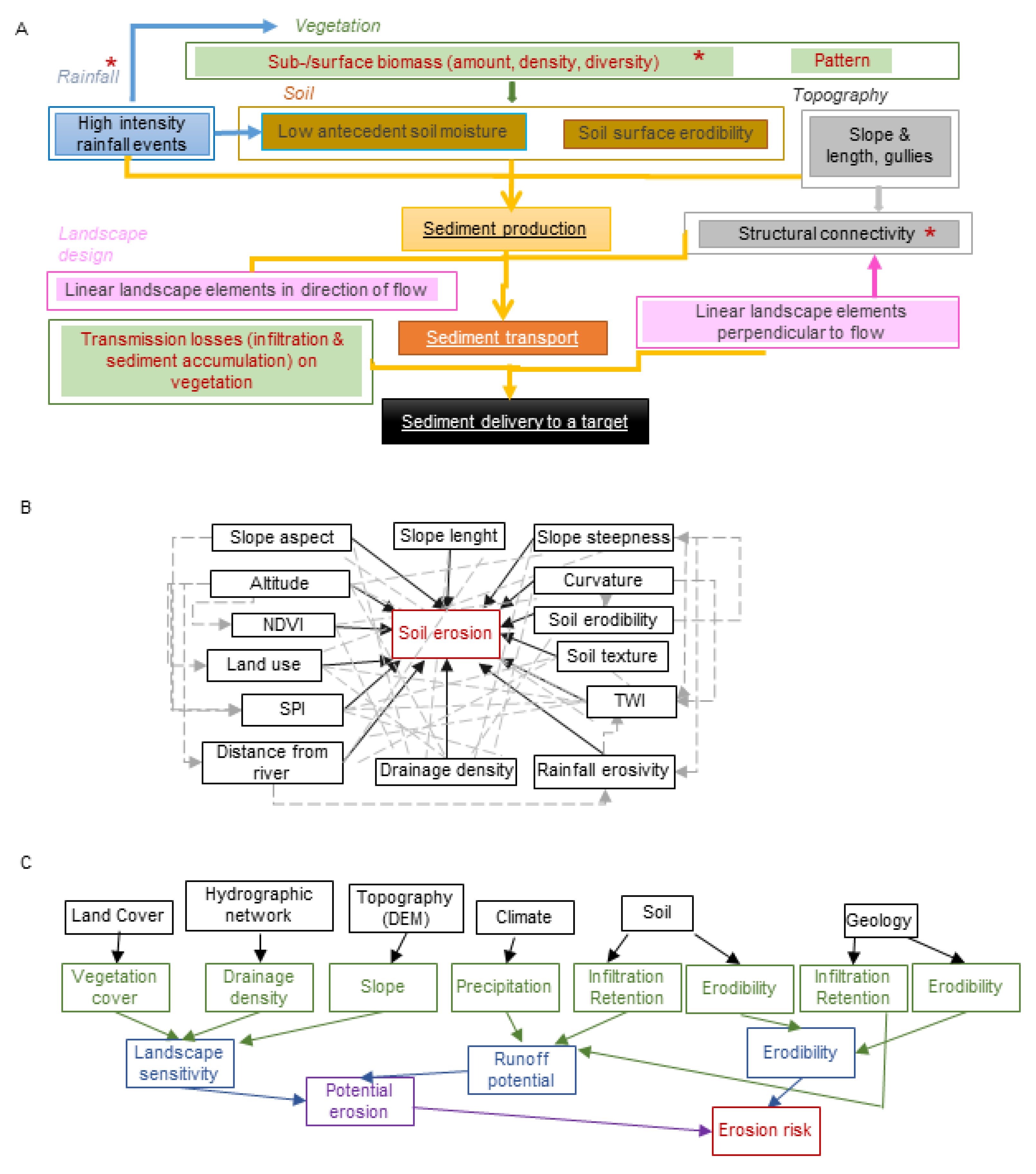
3. Mapping Approaches under Constraints of Data Unavailability

Mapping sediment management hotspots requires conceptualizing of: (i) processes causing erosion (sediment production), transport (sediment delivery), and accumulation (deposition or sedimentation); and (ii) identifying and describing of functional relationships between processes and dominant factors in a specific geographic area. Multiple geomorphic processes are leading to reservoir siltation, e.g., runoff or subsurface-flow induced water erosion, wind erosion, or mass processes, such as landslides.
Mapping erosional hotspots for management is spatially and temporarily scale dependent. A single map of erosional hotspots is simply a snapshot of the state (current or future) of coupled natural-human system and represents a combination of potential and actual properties. On each scale (for example, a hillslope or catchment; event or year), and each resolution (e.g., 1 m, 30 m, or 1 arc sec) different system properties and functions can be analyzed [30,31]. The results of mapping are further dependent on technique, spatial distribution of observation points, and maintaining measurements/records for adequate temporal scales [25,32,33]. Therefore, conceptualizing sediment hotspot mapping for management requires clarified aims, which help define dominant processes (e.g., hillslope erosion or sediment delivery to reservoir); spatial scales, which help to define the area of interest and appropriate resolution (e.g., particular hillslope or catchment above reservoir); and temporal scales, which help to define period of interest and appropriate resolution (e.g., long-term mean, seasonal, and actual state after an event).
Figure 2A conceptualizes the sub-processes leading to sediment delivery in semi-arid landscapes, and their controlling factors. In this example, the dominant controlling factors are: (i) rainfall properties; (ii) soil properties; in interaction with (iii) vegetation properties; (iv) topography; and (v) landscape design (the patterns of artificial or natural linear landscape elements and land uses). Hereby, sediment production and transport through landscape rather than runoff generation and propagation through landscape are in the focus, without considering the sediment production and transport in permanent streams. The occurrence of high intensity interval rainfall events, which are linked closely to peaks in sediment delivery [34,35]. Density and diversity of above-ground and sub-surface (roots) biomass influence infiltration, while vegetation patterns impact infiltration and connectivity of water and sediments in the landscapes [36,37,38,39,40]. From soil properties, the erodibility of soils and antecedent soil moisture are considered in Figure 2A, whereby specific catchment conditions may reflect the effects of other soil properties on runoff generation and particle detachment, i.e., duplex soils, content of shrinking clays, hydrophobicity, and/or exposure of parent material or subsurface soil horizons with erodibility differing from surface soil horizons [41]. Topography affects the sediment production via hillslope inclination and length (Figure 2A) and sediment transport by influencing structural hydrological and sediment connectivity via surface roughness [42]. Finally, landscape structure (spatial organization of landscape elements and land uses) can enhance, modify, or retard sediment transport. Other factors (see, e.g., [16,43] and Figure 2B,C) can be chosen to represent the model of physical reality.
The type of data that are selected, measured, or analyzed for particular spatial and temporal resolutions will be heavily influenced by the concepts/ideas that each researcher is attempting to map. For example, the relationship between controlling factors of sediment delivery could be represented in multiple ways. Firstly, expert knowledge can be applied to determine qualitative decision rules and hierarchical organization of controlling factors [16]. Alternatively, statistical approaches can be used [24,34,44,45,46]. Other approaches include empirical models (mainly Universal Soil Loss Equation—USLE, or Revised Universal Soil Loss Equation—RUSLE) [14,18,20,22,23,47], or physically-based models. either spatially distributed or spatially lumped (e.g., Soil Water Assessment Tool—SWAT [12,48,49,50] and Water Availability in Semi-Arid environments-SEDiments—WASA-SED [51]).

4. Leverage Areas for Sediment Management

To address some methodological aspects of hotspot mapping for dam sediment management, we provide an example for leverage areas mapping under constraints of sparse data in two semi-arid catchments described below.

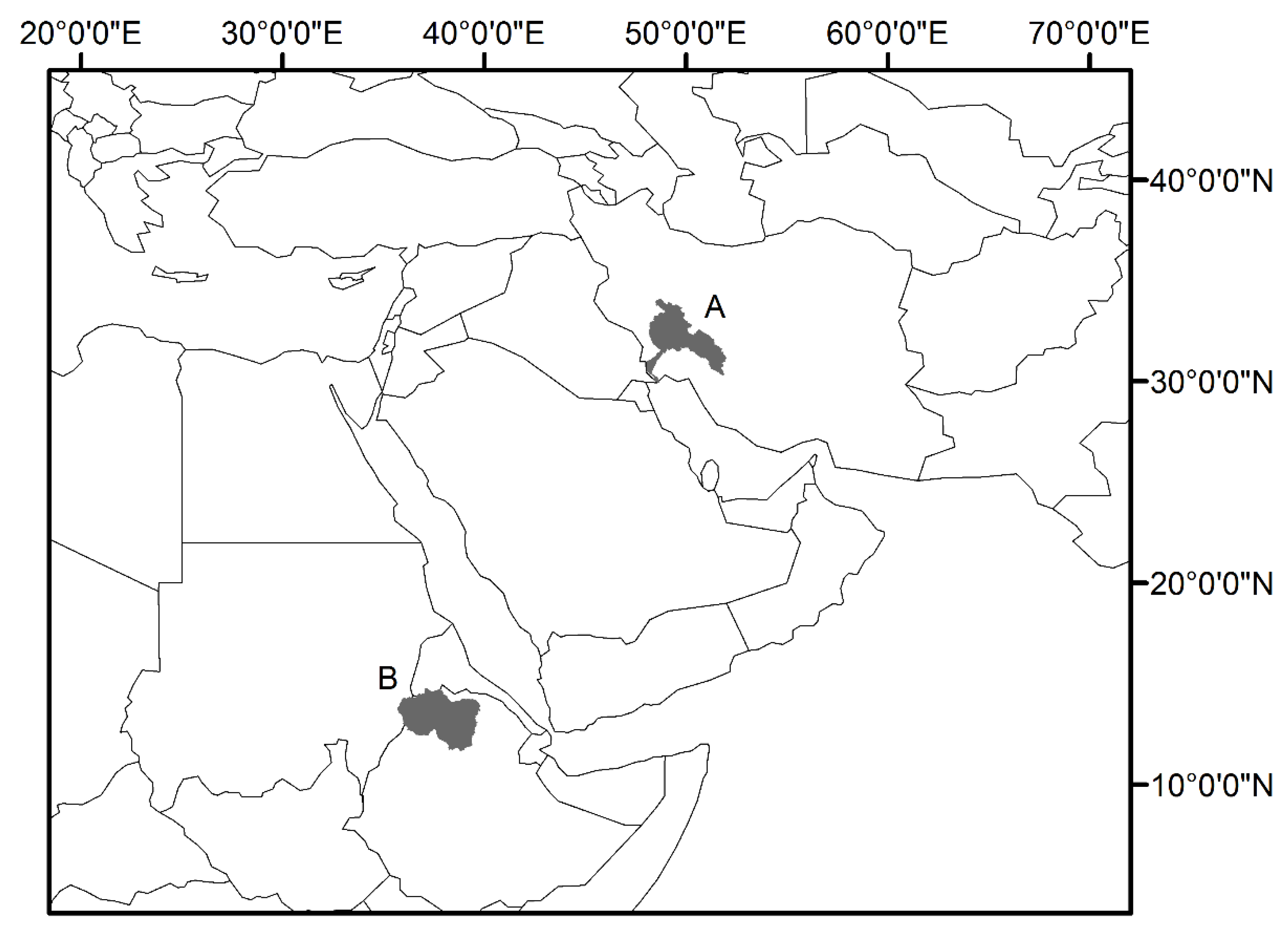
4.1. Case Study Areas

Two study areas were Karun in southwest Iran and Upper Atbara, which spans southeast Sudan, north Ethiopia, and Eritrea (Figure 3 and Table 1). Karun—the most effluent river in Iran—has its source in the Zagros Mountains. River flows are westward towards the Persian Gulf Basin, where it enters near the Euphrates and Tigris confluence (Arvand Rud/Shatt al-Arab). The Karun catchment (~66,600 km2) has many sub-basins (e.g., Koohrang and Dez) with multiple operational dams (Karun 1–4, Gotvand, Dez, Ludbar Lorestan, and Kamal el-Saleh Dams). The catchment has an arid desert hot climate, with most rainfall falling November to March [52,53]. The Upper Atbara catchment (~95,750 km2) is located in the northern part of Ethiopian Highlands. It can be subdivided into two sub-basins: Setit/Tekeze River and the Atbara River, which flow into the reservoir of Upper Atbara and Setit Dam complex shortly before their junction (Table 1). The climate is temperate in the south and southeast, with increasing aridity towards the north, where arid steppe hot climate prevails [52]. Most precipitation falls during a rainy season between May and September [53]. In both regions, shrub and tree cover prevail at highest altitude, which transition to grasslands with rain fed agriculture. The driest areas in Karun basin are bare, sparsely to non-vegetated [54].

4.2. Data Inventories

The minimum data inventory was represented by selecting data available from global repositories and published literature. The accessible data inventory was established during two years of continuous stakeholder involvement in cooperation with local scientists and water management authorities (Table 2). In both regions, it was not possible to find local data covering the entire area of interest at finer resolutions than datasets available in the minimum inventory. Meteorological and hydrological monitoring data were available for some Karun sub-catchments, while no more detailed data were available for soils and vegetation. Several land use maps available at global scales [54,59] provided differing spatial distribution of land use classes, crop types, and irrigation agriculture. In both case study areas, no land use maps with spatial coverage comparable to global datasets were available, with information mostly restricted in agricultural areas. Contrary to local data, the metadata information (e.g., acquisition date and mapping methods) was available for global datasets, which made them more suited for approaches aiming to tackle spatial-temporal process dynamics. The global data best representing reality were selected based on expert opinion of water authorities and scientists [54].

4.3. Methods

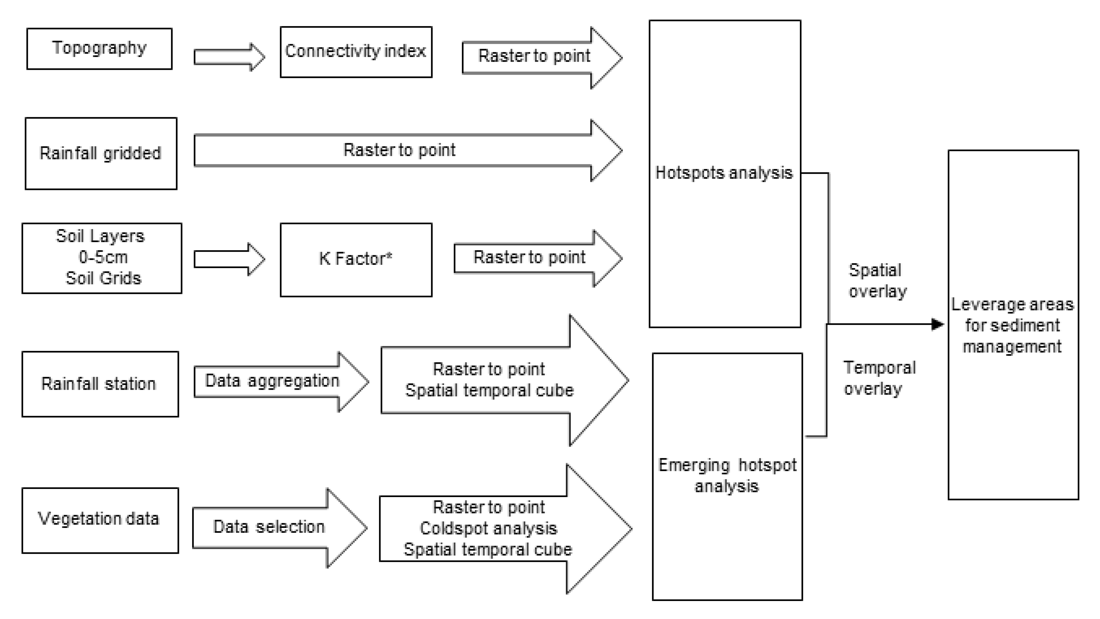
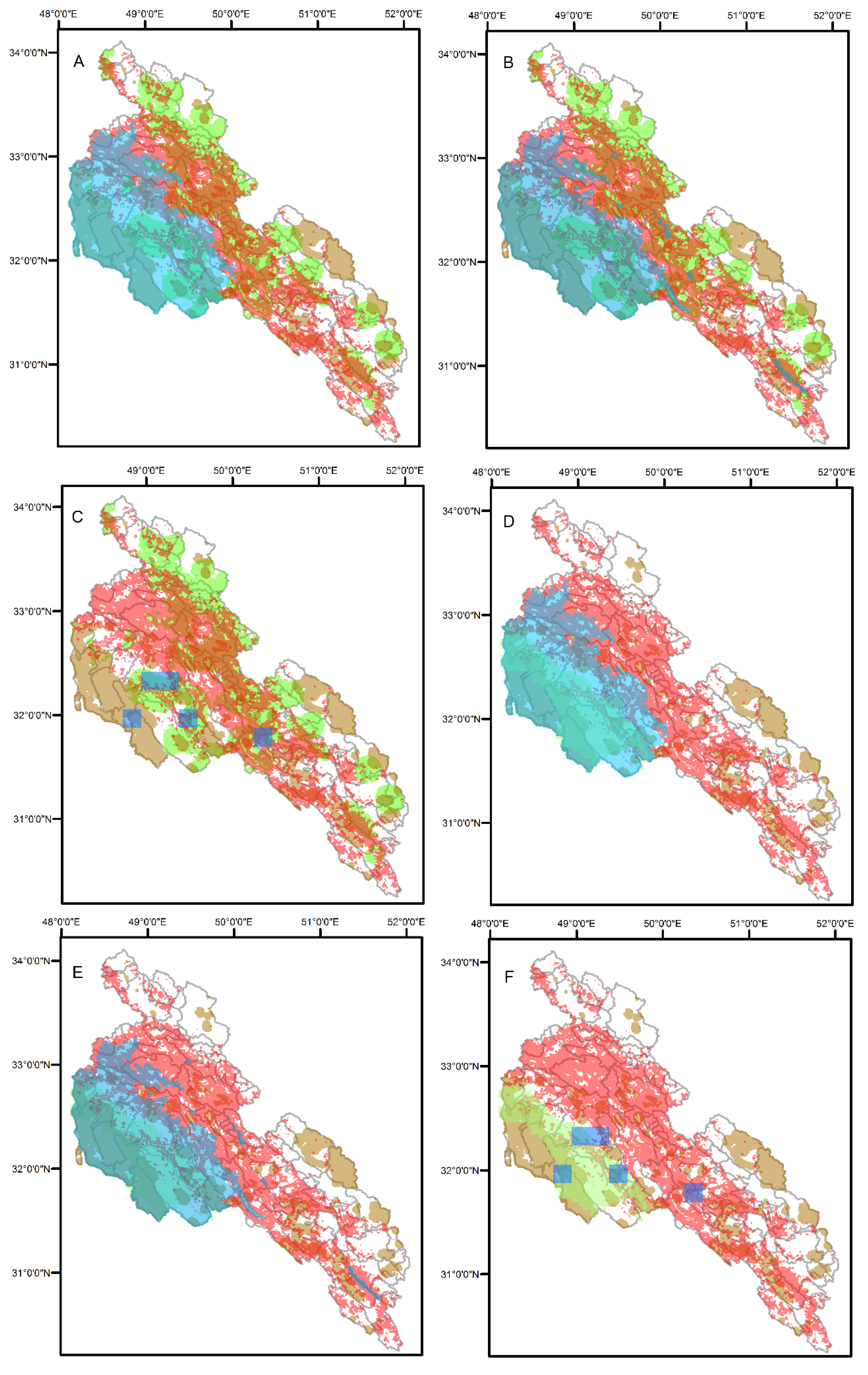
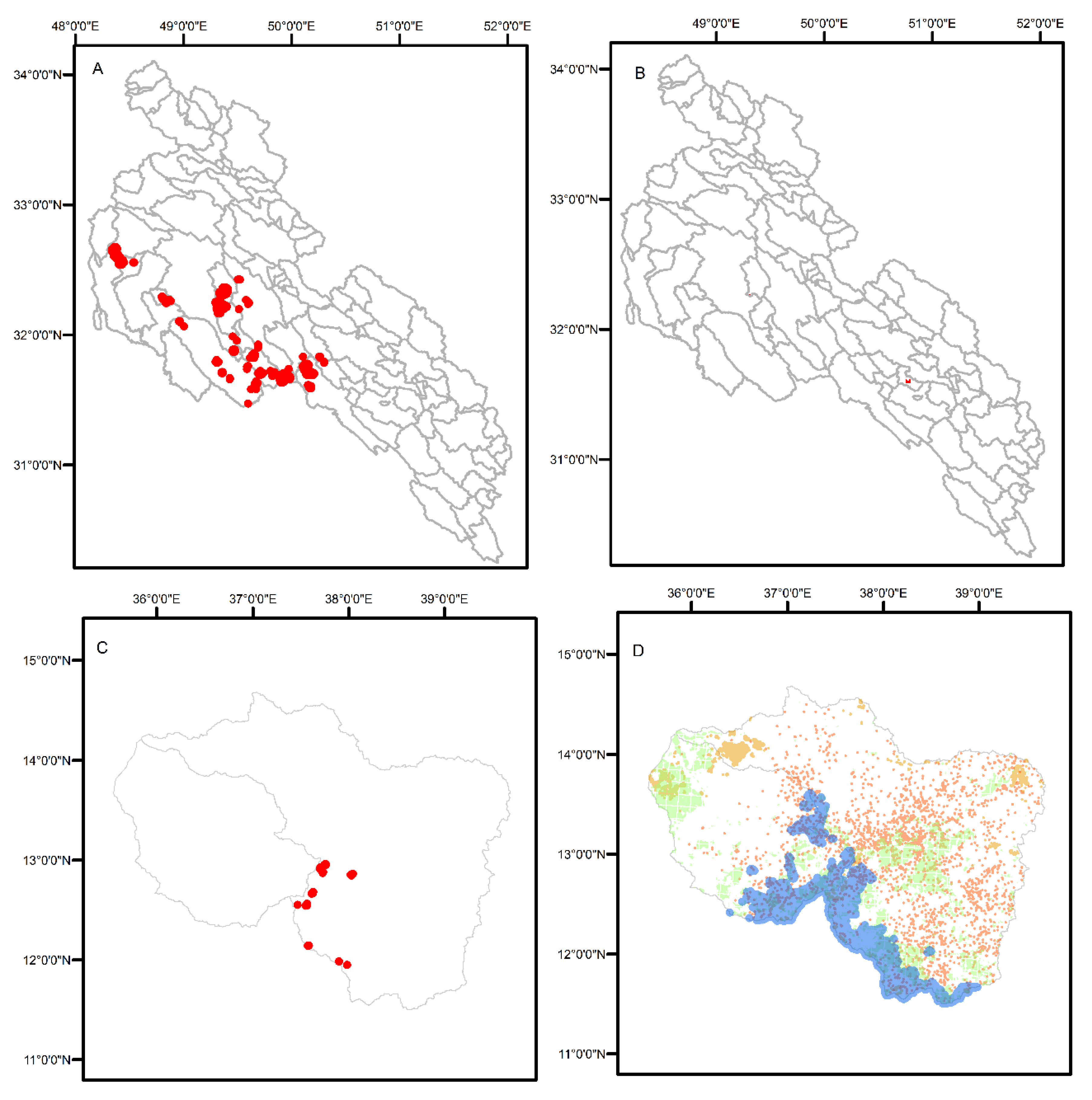
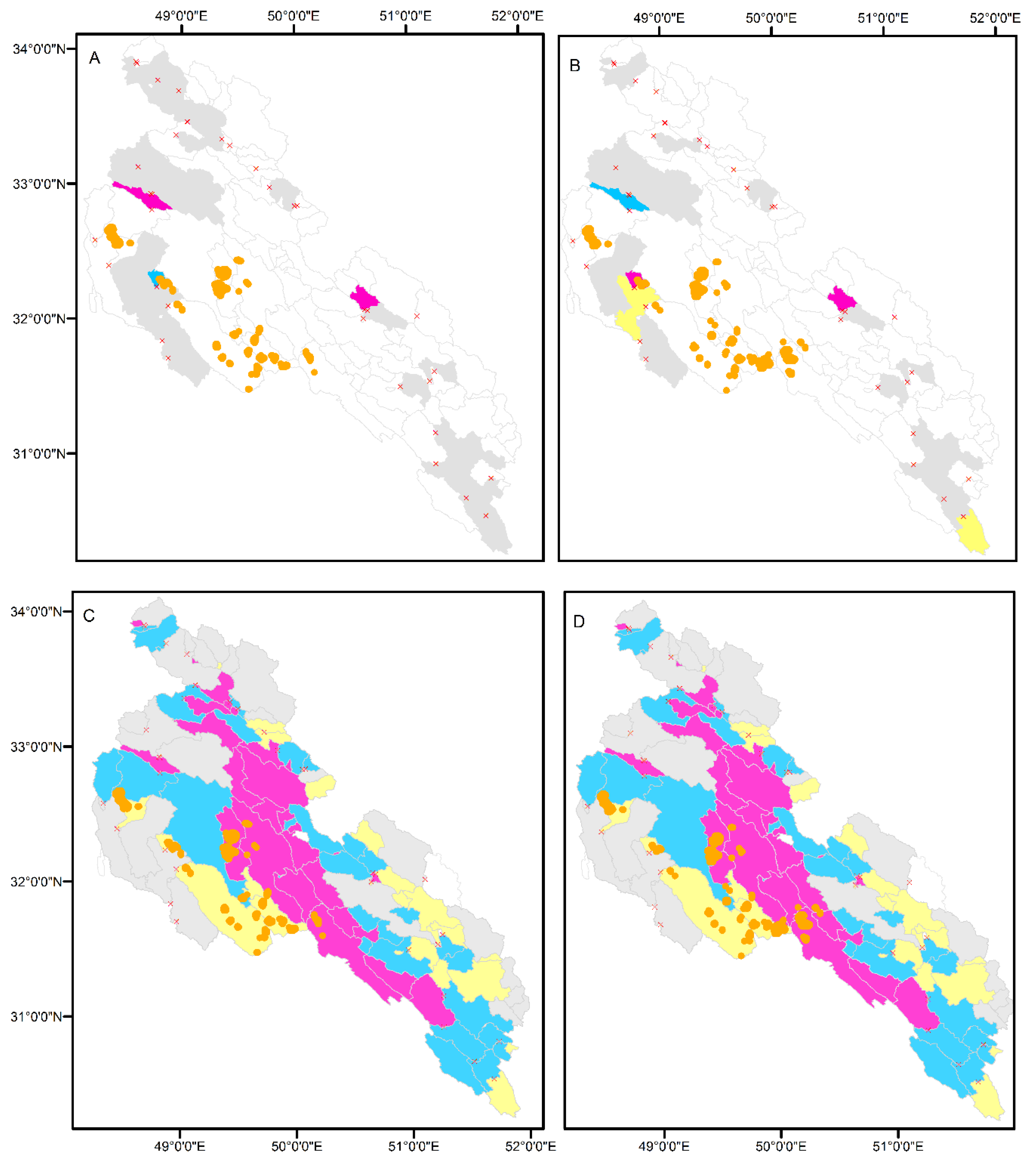
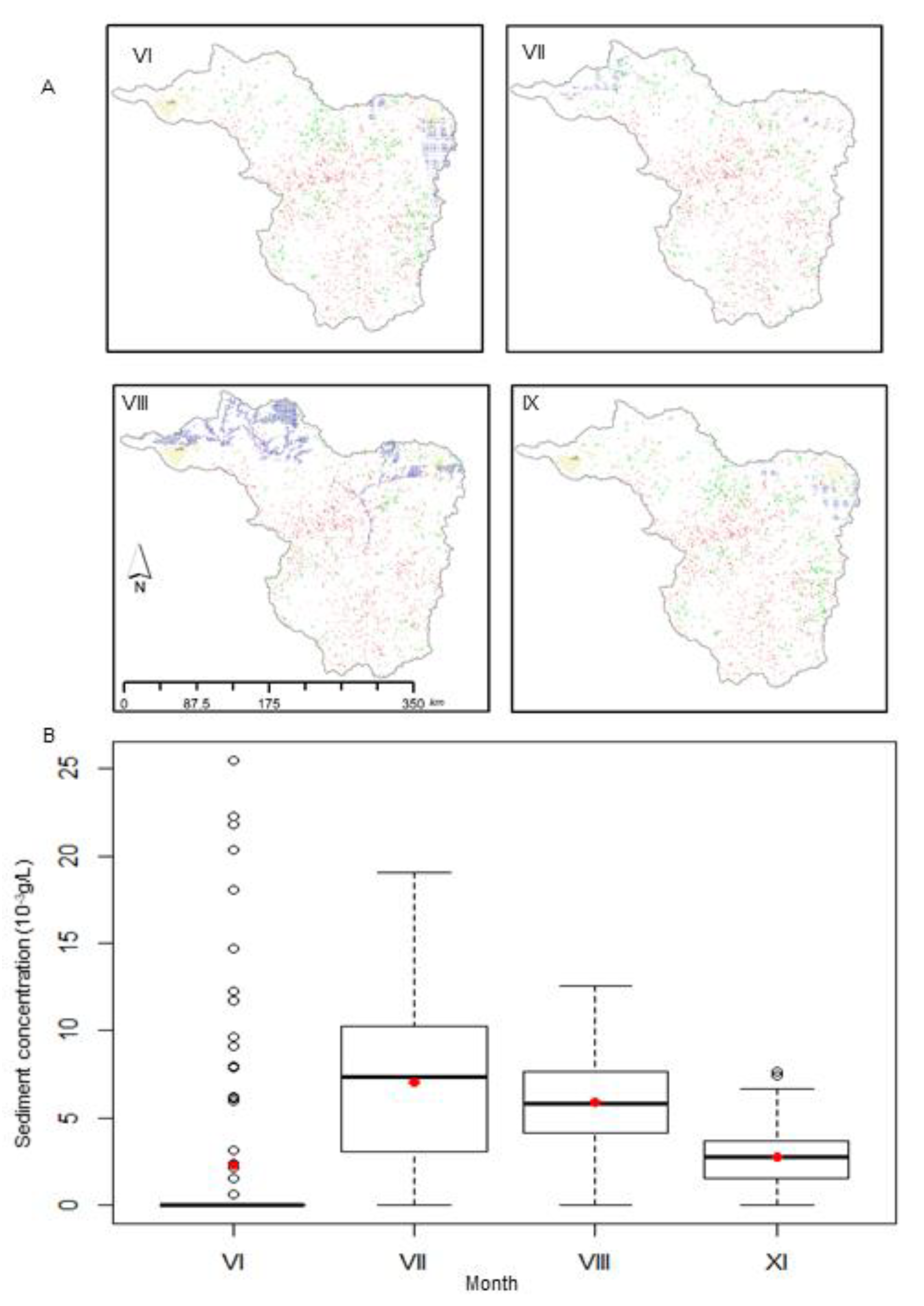
4.3.1. Mapping Approach

Previously, we showed that different data inventories influence differences in spatial and temporal accuracy of representations of physical reality, and that a range of methods can be applied to high quality datasets. However, to demonstrate the effect of different inventories for mapping of erosion hot spots, basic GIS mapping methods were chosen. To do so, we used the conceptual approach visualized in Figure 2A, where red asterisks indicate the considered variables. The inputs for our analysis (Table 2) were processed as shown in Figure 4.
The hotspots and emerging hotspots were calculated using Getis-Ord Gi* [64,65] statistic in ArcGis 10.4. This geostatistical approach allowed distinguishing areas where features with high (hotspots) or low (cold-spots) values were surrounded with other features with high (low) values. Each feature was compared to its neighborhood, and each neighborhood sum with the sum of all datasets. The emerging hotspots were analyzed in spatial-temporal domain. The analysis allowed distinguishing whether hotspots are stable, emerging, or diminishing in relation to given point of time.
Topography data [55] were pre-processed as required for connectivity index calculation [42,66]; surface roughness was used as weighting factor. We calculated connectivity index to targets—dams and rivers (vectorized from Q Gis and Arc Info Base Maps). The connectivity index map was aggregated (by factor 30, median technique, providing pixel size ~900 m) to decrease the number of points for hotspot analysis ([64,65] ArcGis 10.4). The setting for spatial conceptualization of relationship was fixed-threshold distance, which means that effects of neighboring features diminish with distance. The Euclidean distance (connecting two points with a straight line) was chosen as distance calculation method. We applied false discovery rate correction (ArcGis 10.4), which reduced the critical values of statistical significance (p) due to spatial dependence. Hotspots identified by 95% confidence provided the final output (settings: GiBin > 2, GiZScore > 0, and GiPvalue < 0.1).
Soil Grid [58] layers (1 km)—silt, clay, and loam—were used to calculate texture [67]. Texture, together with GIS layers (dominant soil type, organic matter, and coarse sediments), was used to calculate K factors using previously published methodology [68]. An African soil map [61,62] was used for soil types in Upper Atbara. The hotspot analysis and selection followed the above-mentioned settings.
Rainfall station data from Karun (2000–2016; 29 stations; 15 hydrological years) were aggregated to monthly rainfall depths, and a shape file containing station location and the corresponding number of data points was used to build up spatial-temporal cube (settings: time step: 30 days; distance interval: 20 km; and summary fields: max, mean, sum, and med). These were included in an emerging hot-spot analysis ([63,64] ArcGis 10.4; settings: neighborhood distance: 60 km; neighborhood time step: 1; and statistically significant hotspots selected: GiZScore > 0, GiPvalue < 0.1, and GiBin > 2).
Vegetation data [63] were selected to visually represent maximum spatial distribution of low NDVI values (at the end of the season, or in December or May) from time-series 2000–2016. Afterwards, we filtered out negative values (no ecological meaning), and focused on point values from which hotspots were calculated. Statistically significant cold-spots (setting: GiPValue < 0.1, GiZScore < 0, and GiBin > −2) were selected, turned into points, and spatial-temporal cubes (time step: 1 year; and distance interval: 1000 m) were built for emerging hotspot analysis ([64,65,69] ArcGis 10.4). Statistically significant hotspots (GiZScore < 0, GiPValue < 0.1, and GiBin > 2) were selected for remaining hotspot analyses (connectivity index, gridded rainfall data, and K factor). In emerging hotspot analysis, the “last step” was to define the targeted temporal overlay (e.g., end of December).
The leverage areas represented the spatial-temporal overlay of hotspots or emerging hotspots of four controlling variables. Only statistically significant hotspots and emerging hotspots of the four controlling factors (with >90% probability of occurrence) where overlaid. For the spatial intersect, a buffer of three times the minimal layer spatial resolution (3 × 1 km) was allowed.

4.3.2. Validation Approach

To discuss challenges in validation procedure, spatial distribution of erosion hotspots was compared to observed or modeled sediment yield in Karun. Sediment data from sediment monitoring stations (39) in Karun consisted of continuous measurement with frequency of mostly one day in a month between October 1999 and September 2012. They were considered to represent monthly sediment volume, and, if more measurements were available in a month, cumulative value was considered. We calculated area-specific sediment yield (Mg km−2 month−1) for each measuring station. Consequently, long-term mean from annual mean values and long-term sediment yield in December were related to spatial distribution n of hotspots.
Modeled values of daily sub-catchment sediment yield were obtained by using WASA-SED, a freely available deterministic, process-based, spatially semi-distributed, and time-continuous hydro-sediment logical model, specially developed for semi-arid landscapes [70,71,72,73,74,75,76]. Data pre-processing included: (i) interpolation of reanalyzed of global-gridded daily time-series of air temperature, precipitation, relative humidity, and short-wave radiation for the time period 1950–2018 [60,77] using previously described methods. [78]; (ii) reclassification of land cover map [54] into nine classes; (iii) vegetation parameterization after [51,69,72,79,80,81,82]; (iv) preparing soil map and soil parameters based on SoilGrids [58,83]; and (v) landscape discretization based on SRTM digital elevation model, vegetation and soil map [75,84]. Unit sedigraph approach was used to calculate sediments, and groundwater below soil zone and snow routine were applied [85]. A model pre-run (1 January 1950–31 December 1979) provided initial conditions (water, snow, and sediment) for the actual model run for the time period 1 January 1980–31 December 2018.

5. Addressing Methodological Aspects of Hotspot Mapping for Dam Management

5.1. What to Map: Means or Extremes?

Maps are some diagrammatic representations for a system’s state during the mapping period, for a particular spatial scale, while it remains unchanged. Variability of slow (e.g., soil texture), fast (e.g., soil moisture and rainfall volume), and emerging (connectivity) system variables, and the relations between them, change at different rates and intensities. If a map is used for decision making, it is preferable to define the conditions for which the map represents, and, when possible, represent multiple possible system states, conditions, and behaviors. Such an approach is well established for flood risk mapping, which displays various spatial distributions for floods of different recurrence intervals, or distinguish seasons in which flooding can occur. To our knowledge, this is rarely the case in sediment management. For example, studies showed that amount of sediment leaving a catchment at its outlet (furthermore, sediment yield) is closely related to rainfall seasonality and rainfall extremes in semi-arid catchments (e.g., [35,86]). However, the relation between rainfall amount and sediment yield is not linear, while redistribution of sediment in catchment or in river channel influence sediment yield when the catchment is well connected during the event. Therefore, ideally a manager of a dam would be aware of sediment production areas, temporary storage areas, and connectivity in their catchment, and consider their spatial-temporal dynamics. For this, modeling approaches that distinguish long-term means and extreme rainfall conditions, or hindcasting long-term trends, can be useful. Ideally, modeling would be applied for strategically planning management for upcoming seasons [10,87,88]. Again, availability of data inventories for continuous model calibration and validation, availability of seasonal rainfall predictions, and modeling (labor, financial, time, and programming) costs hinder the application of more complex models at large scales. Seasonally variable mapping cannot substitute for precise modeling approaches, but can provide more detailed information in comparison with those using mean conditions (e.g., long-term average rainfall). Seasonal rainfall volumes and vegetation state derived from remote sensing (e.g., Sentinel-1, Sentinel-2 I/II) are examples where it is possible to incorporate variable controlling factors. Figure 5 provides an example of spatial-temporal datasets based on different inventories in Karun (Iran). Minimum data inventories based on global raster datasets were applied for rainfall (Figure 5A,B,D,E), structural connectivity, soil erodibility, and vegetation. The rainfall data inventory was based on station-based long-term measurement of rainfall (Figure 5C,F). Three-possible representations of rainfall data were documented. Rainfall data in Figure 5B,E represent hotspots of mean yearly rainfall erosivity, and rainfall data in Figure 5A,D reflect hotspots of monthly rainfall depth in the rainiest month. The highest rainfall monthly depth was reached in January according to global data (Figure 5A,D) [53], while analyzed station data showed it was December. Spatially and temporarily significant hotspots based on station data (points, not interpolations) at the end of the last analyzed hydrological year (September 2016) provided more detailed results, but were limited in spatial validity/extent.
Another temporal dimension is provided by the vegetation data, which represents areas where the lowest biomass repeatedly occurred at the beginning of a growing season (end of October during 2000–2016), and approximately one month later when the rainiest months started (beginning of December, during 2000–2016). Temporal discrepancy of overlaid rainfall and vegetation hotspot maps was intentionally introduced to demonstrate the necessity of evaluating the temporal validity of input sources, and to select the appropriate time periods relative to application of management measures. Figure 6 shows leverage areas for sediment management derived from matching temporal sources—global data of monthly rainfall and vegetation in December (patterns relative to beginning of December 2016; Figure 6A), station-based rainfall, and MODIS-based vegetation (both patterns) relative to end of October 2015 (Figure 6B). In the first example, the vegetation, soil, and connectivity hotspots are likely to occur before the December rains (annual peak in rainfall volume). This information can be used to prepare for ad-hoc sediment capture measurements in upcoming months. The latter example reflects leverage areas for sediment management surrounding rainfall monitoring stations. They cover areas where statistically significant high soil erodibility and high connectivity are located. Additionally, statistically significant spatial-temporal hotspots of rainfall and low vegetation cover repeatedly occurred there in the last 15 years (October 2000–October 2015). This map can assist sediment management by identifying permanent hotspots in proximity with a measurement station, which continue to be active subsequent periods.

5.2. What to Map-spatial or Temporal Extremes?

Representing spatial-temporal relationships to indicate when minimal management efforts could have maximized effects is desirable [10]. The use of gridded time-series products enables the application of geospatial statistical methods to distinguish spatial and temporal extremes. Many methods can be applied on spatial environmental variables [24,89,90,91], and additional tools are available for mapping changes in temporal trends of spatial data (e.g., [92,93,94,95], and this study). In our study, emerging hotspots (Figure 5 and Figure 6) represent statistically significant relationships of a spatial component, within its spatial and temporal neighborhood. Analysis of spatial-temporal relationships was only possible for factors considered as dynamic (temporarily and spatially variable), and only where appropriate datasets were available within the applied inventory. The connectivity index used highlights how conceptual representations can restrict applicability of analyses to particular spatial-temporal domains.
Availability of a single digital elevation model constrains application of topography-based time series, which can only be derived from multiple digital elevation models (similar to [69,96]). We used surface roughness as a weighting factor for connectivity index calculation, while others [95,97] have opted for temporally changing (remote sensing derived) crop erodibility factor. The latter enabled derivation of a connectivity index time series in order to study vegetation-based changes in connectivity. Computational limitations of applied algorithms [64] at regional scales further limit the applicability of temporal time-series, and therefore the analysis framework can be simplified [95], ideally matching management’s spatial and temporal requirements.

5.3. How to Validate and Prioritize Hotspots?

When mapping sediment hotspots using physically based models, the calibration and validation of model efficiency and sensitivity analysis were well established for cases where input data were available [31,48,98]. Despite the commonality of result validation in modeling studies, it is rather uncommon for hotspot mapping. One can argue that hotspot mapping (model) conceptualization focuses more on potential than actual erosion (sediment production, or sediment delivery), which makes validation troublesome [16]. Generally, two validation approaches are applied in modeling studies: (i) validation using monitoring data; and (ii) multi-model comparison. Use of monitoring data for validation is limited by availability, as well as, in cases of spatially lumped data (i.e., station measurement), by the ability of point measurements (plot or catchment outlet sediment yield) to describe spatially and temporarily distributed processes such as sediment cascades [16,99]. The same is valid for the mapping approach itself, and therefore caution should precede selecting appropriate variables and temporal snapshots for comparison [33]. For example, a long-term annual mean sediment yield measured at catchment outlet (during 2000–2013) is compared to leverage areas for sediment management at the end of the dry season (September in 2000–2016, Figure 7A), and December leverage areas are compared to long-term December mean (Figure 7B). To show spatial extremes, a heat map of spatially lumped long-term means of area-specific sediment yield from outlet measurements (represented as one value in entire catchment area) are compared to spatially and temporarily significant spatially distributed data (leverage areas).
However, such comparisons are dubious, as most catchments with identified sediment leverage areas lack sediment data measurements. In the study area, spatial distributed information of eroded/eroding areas (such as soil profile truncation maps, rills, and gullies maps) were unavailable, and therefore validation by geostatistical methods [17,100,101] was not applied. An alternative to validate results is to compare result with one or multiple models [102], as shown in Figure 7C,D. In these figures, leverage areas are plotted against heat maps of modeled, spatially lumped long-term means of area-specific sediment production on hillslopes.
The advantages are full spatial coverage of modeling results across the entire catchment where no data were available. Visual relations between hotspot areas with the upper quartile of sediment yield for each catchment is stronger than in Figure 7A,B, but high area-specific sediment production was modeled also in catchment were no hotspots were detected. Non-calibrated model runs were used for this comparison in order to point out possible misuse of modeling approaches in data sparse regions. Even though graphical validation of observed versus modeled (discharge and sediment load in river) values showed relatively good process representation for naturalized flow, the results themselves should be taken with caution and further compared with calibrated model. Under constraints of availability, caution should be paid to data pre-processing; model validation should go beyond model performance coefficients, and uncertainty introduced by missing data carefully considered and discussed [103].
A third possibility for validating mapping results where no validation data exist is an assessment by local expert knowledge or participatory mapping [20,21,104]. Accuracy of participatory mapping approaches is, among others, limited by: (i) diversity of definitions and approaches to participatory mapping; (ii) spatial attributes measured in participatory mapping; (iii) sampling, participation, and data quality; and (iv) relationships between participatory mapped attributes and physical places [105]. It further requires active stakeholders’ involvement (Figure 1), and its application for the study areas is a topic of ongoing discussions with Sudanese partners.
The primary motivation of risk, hotspot, or leverage area mapping is to support decision making in water and land management, thereby providing means to prioritize hotspots areas through data analysis and/or visualization [106]. While the decision to prioritize management is in the competence framework of responsible stakeholders (including institutions), scientific results can support multiple decision support frameworks [107]. Scientists can assist hotspot prioritization for variables and scales they considered in their analysis in order to identify the temporal and spatial domains when/where action is required. Local knowledge or short-term lumped data series can be compared to mapping outputs relative to a point of time, for prioritizing timescales and areas for ad-hoc management interventions (Figure 8).
Furthermore, environmental and societal factors can be used in analyses targeted at soil and water conservation measures [20,102]. Prioritization was performed in multiple ways:
  • ordinary decision rule matrix [16];
  • threshold-based prioritization [20];
  • value-based classification, including heat maps or percentiles (e.g., [49] and Figure 7);
  • geostatistically-based prioritization (e.g., statistic in spatial-temporal domain, [69,95,97], this study).
In doing so, the stakeholders’ aims and spatial and temporal scales of interests should be considered [108,109,110].

6. Common Challenges for Research and Management of Leverage Areas with Sparse Data Availability

In previous sections, we discuss how a lack of available data limit identification of sediment source areas contributing to reservoirs siltation. We review existing approaches and develop a simple method using a minimum inventory of globally available datasets that can be applied in situations where additional precise data are available to enable physically-based modeling. We present a simple mapping approach that builds upon latest advancements in understanding connectivity as a factor of sediment delivery [111,112,113,114,115].
Our work highlights how lack of data availability limits the mapping in multiple ways. Firstly, data can limit understanding of controlling factors of sediment delivery and relationships between controlling factors. Despite good understanding of functioning of bio-physical systems in semi-arid areas [37,38,116,117], local eco-hydrological and eco-geomorphological conditions can stimulate specific catchment sediment responses [118,119]. Regional studies showed that rainfall-discharge-sediment response curves and some of the controlling factors varied among catchments and/or seasons [14,35,44,120]. Events of similar magnitude can deliver differing amounts of sediment if intra- or inter-event catchment connectivity changed, or stored sediment was released within an event [121]. Simplifying existing relations or underrepresentation of some processes in favor of others is a recognized issue in mapping and modeling studies, and limited data availability can pose additional challenges [31]. Simplifications can be introduced by considering elementary factors with general, but possibly not site-specific, influences on sediment delivery (e.g., our approach). Alternatively, controlling factors lacking explanatory power in the environment can be derived and mistakenly taken into consideration.
Secondly, data availability limits the spatial and temporal scale over which landscape can be represented and understood. The globally available remote sensing or gridded products (meteorology, soils, etc.) have a great information quantity and quality, and undisputable spatial-temporal information distribution. However, ground truthing is necessary to fully utilize their potential for applications such as classification of land use, crop cover, and phenophases [122,123]. Similar to digital elevation models, remote sensing products (and derivate such as in this study) have a defined resolution that can lead to misrepresentation of processes occurring on sub-grid scale [17,124,125], which in turn can limit management at sub-grid scales. For example, most sediment management measures applicable in sediment source areas, such as check dams, buffer strips, soil cover management (crop, land use change, and geotextiles), terracing, and others [17,126] would ideally be planned at fine scales as leverage areas, to be distinguished from global datasets. Recent developments may enable researchers to use fine-resolution remote sensing products such as Sentinel-2, with coarse-resolution data (up to 10–20 m) in the near future. Such methods were not applied here because we lacked sufficient time series data (acquisition started in 2015). Spatial resolution is further important if scale dependent variables (e.g., slope and flow path length) are analyzed [17,69,127]. Therefore, the scale should be carefully matched to the analysis purpose. This will differ for regional scale mapping focused on distinguishing dominant sediment sources in contrast to developing area-specific management plans. Additionally, when detailed scales are considered in management support systems, the usability of minimum inventory (global available datasets) decreases.
Third, data availability can limit the applicability of advanced scientific methods, and possibly validation of results. Comparing models or methods can sometimes substitute for validation or provide results that are more complex. However, the following should be considered: (i) Many existing approaches consider similar variables and physical representations between them [31]. (ii) Although many models are available that account for all known influential variables, coarse data resolution, poor precision or quality, and/or general availability may limit their usage. One example found herein was the rainfall intensity and associated kinetic energy as a crucial variable leading to sediment detachment. During a rainstorm event, rainfall intensity changes several times [128], but daily aggregates, or maximum 30-, 15-, or 6-min intensities are used to calculate rainfall energy in soil erosion models, while more fine-scale data on intensity variability are not available.
Many approaches have been developed to tackle challenges posed by data unavailability. These include new acquisition methods, new models, and performance metrics development. Their development and application in land degradation research and other fields has grown in recent decades ([129], this study). However, in the current era of data-driven science where terabytes of information are collected every second, some key components are still missing. This reflects institutional barriers or simply a lack of cooperation in data sharing and data coproduction. For example, water managers often record the quantity of water allocated to agriculture, but lack information on actual distribution among farmers and fields, as well as the actual groundwater withdrawal. Additionally, managers lack information on field management practices, such as seeding/planting terms (influencing plant cover of soil, evaporation changing as plant grows, etc.), amount of fertilizer, or number of cattle breeding on semi-natural pastures, which all contribute to land and water quality degradation. Multi-factor character of many environmental problems is well acknowledged in science, but not reflected in institutional structures and institutions’ cooperation networks in many countries, and transboundary basins [35,130,131]. The call for transdisciplinary research in the land degradation community has existed for a longer time, all the while acknowledging the need to address societal challenges is evermore present. Despite this, data sharing, open-source publishing, and truly inter-sectoral and transdisciplinary research projects are still uncommon scientific practices [29,132,133,134].
Researchers and managers are hereby invited to define the temporal and spatial scales over which land degradation and/or water balance should be managed. Furthermore, we encourage open, sharable, and suitable data acquisition, which support development and application of methods that do not omit or simplify complexity and inter-scale characteristics of environmental issues linked to sediment delivery.
Another point raised during this study is how management considers spatiotemporal patterns of sediment delivery and its controlling factors. In other words, in both research and management it is necessary to account for the continuously changing nature of coupled socio-ecological systems, as well as compounding non-linear responses of landscape systems [135]. In our continuously changing world, sediment management is likely to fail if it continues to target long-term mean values rather than variability. Sediment management might fall behind ongoing and future environmental trends if it continues to omit in the most influential factors and their compound effects [128,136]. Eco-hydrological hindcast modeling for water and sediment management [87,88] provides a step forward for addressing management challenges related to ongoing change. While ecosystem stewardship principles [137] that focus on preserving system functions are well-suited for reservoir sediment management, complex and systemic action needed to apply such principles are in direct conflict with multiple barriers described in the study.
Therefore, spatial-temporal trends analysis of socio-ecological hazards related to reservoir siltation must be included in risk-mapping context. Furthermore, examples (such as in this study) discussing the impacts of data unavailability on applicability of state-of-the-art scientific methods in management context need to be discussed in the context of sustainable management of socio-ecological systems from the perspective of both scientists and managers.

Author Contributions

Conceptualization, A.S.; acquisition of measured data, M.A.S. and F.R.G.; data processing, M.Z. and M.M.; methodology and analysis, A.S. and A.M.; Writing, A.S.; revision process, A.S.; stakeholder dialogue, A.S. and M.Z.; and comments and edits, A.M., M.Z., and M.A.S. All authors have read and agreed to the published version of the manuscript.

Funding

This work was funded by BMBF Project 02WGR1421A-I (SaWaM). The APC was covered by the Open Access Publication Fund of TU Berlin.

Acknowledgments

The authors acknowledge the support of Eva Paton (Technical University Berlin), who created the first concept of the erosion hotspot analysis for the project. We thank Axel Bronstert (University Potsdam) for his comments on manuscript. Hooshang Hassounizadeh, Mehrdad Taghian (both Khuzestan Water and Power Authority), Eng. Behron Dibrani (Lahmayer International), and Eng. Mohammed Saleim (DIU) are acknowledged for their help. We are thankful for fruitful discussions with scientists and practitioners in Iran, Sudan, Brazil, Tunis, Algeria and Marocco. We appreciate the much inspiration provided by a growing number of anonymous academic and non-academic stakeholders who openly share their data, discuss their approaches and pitfalls, and bear with the challenges of open, transdisciplinary, and inter-sectoral research projects or science-policy dialogues.

Conflicts of Interest

No conflict of interest to declare.

Data Availability Statement

The data used in this study are publicly available, and cited in the reference section. We regret to inform readers that we cannot share station-based data applied in this study due to property rights and agreements between project parties.

References

  1. Syvitski, J.P.M.; Vörösmarty, C.J.; Kettner, A.J.; Green, P. Impact of humans on the flux of terrestrial sediment to the global coastal ocean. Science 2005, 308, 376–380. [Google Scholar] [CrossRef] [PubMed]
  2. Cooper, M.; Lewis, S.E.; Stieglitz, T.C.; Smithers, S.G. Variability of the useful life of reservoirs in tropical locations: A case study from the Burdekin Falls Dam, Australia. Int. J. Sediment Res. 2018, 33, 93–106. [Google Scholar] [CrossRef]
  3. Rahmani, V.; Kastens, J.H.; DeNoyelles, F.; Jakubauskas, M.E.; Martinko, E.A.; Huggins, D.H.; Gnau, C.; Liechti, P.M.; Campbell, S.W.; Callihan, R.A.; et al. Examining storage capacity loss and sedimentation rate of large reservoirs in the central, U.S. Great Plains. Water 2018, 10, 190. [Google Scholar] [CrossRef] [Green Version]
  4. Zarfl, C.; Lucía, A. The connectivity between soil erosion and sediment entrapment in reservoirs. Curr. Opin. Environ. Sci. Health 2018, 5, 53–59. [Google Scholar] [CrossRef]
  5. El Kadi Abbdelrezzak, K.; Findikakis, A.N. Reservoir sedimentation: Challenges and management strategies. Hydrolink 2018, 3, 66. [Google Scholar]
  6. Liu, C.; Walling, D.E.; He, Y. Review: The International Sediment Initiative case studies of sediment problems in river basins and their management. Int. J. Sediment Res. 2018, 33, 216–219. [Google Scholar] [CrossRef]
  7. Shi, P.; Zhang, Y.; Ren, Z.; Yu, Y.; Li, P.; Gong, J. Land-use changes and check dams reducing runoff and sediment yield on the Loess Plateau of China. Sci. Total Environ. 2019, 664, 984–994. [Google Scholar] [CrossRef]
  8. Nunes, J.P.; Seixas, J.; Keizer, J.J. Modelling the response of within-storm runoff and erosion dynamics to climate change in two Mediterranean watersheds: A multimodel, multi-scale approach to scenario design and analysis. Catena 2013, 102, 27–39. [Google Scholar] [CrossRef]
  9. Mullan, D.; Vandaele, K.; Boardman, J.; Meneely, J.; Crossley, L.H. Modelling the effectiveness of grass buffer strips in managing muddy floods under a changing climate. Geomorphology 2016, 270, 102–120. [Google Scholar] [CrossRef] [Green Version]
  10. Smetanová, A.; Follain, S.; David, M.; Ciampalini, R.; Raclot, D.; Crabit, A.; Le Bissonnais, Y. Landscaping compromises for land degradation neutrality: The case of soil erosion in a Mediterranean agricultural landscape. J. Environ. Manag. 2019, 235, 282–292. [Google Scholar] [CrossRef]
  11. UN WATER. Progress on Integrated Water Resources Management: Global Baseline for SDG 6 Indicator 6.5.1: Degree of IRWM Implementation; UN WATER: Geneva, Switzerland, 2018; p. 69. [Google Scholar]
  12. Welde, K. Identification and prioritization of subwatersheds for land and water management in Tekeze dam watershed, Northern Ethiopia. Int. Soil Water Conserv. Res. 2018, 4, 30–38. [Google Scholar] [CrossRef] [Green Version]
  13. Ben Slimane, A.; Raclot, D.; Rebai, H.; Le Bissonnais, Y.; Planchon, O.; Bouksila, F. Combining field monitoring and aerial imagery to evaluate the role of gully erosion in a Mediterranean catchment (Tunisia). Catena 2018, 170, 73–83. [Google Scholar] [CrossRef]
  14. Gourfi, A.; Daoudi, L.; Shi, Z. The assessment of soil erosion risk, sediment yield and their controlling factors on a large scale: Example of Morocco. J. Afr. Earth Sci. 2018, 147, 281–299. [Google Scholar] [CrossRef]
  15. Alahaine, N.; Elmouden, A.; Aitlhaj, A.; Boutaleb, S. Small dam reservoir siltation in the Atlas Mountains of Central Morocco: Analysis of factors impacting sediment yield. Environ. Earth Sci. 2016, 75, 1035. [Google Scholar] [CrossRef]
  16. Bou Kheir, R.; Cerdan, O.; Abdallah, C. Regional soil erosion risk mapping in Lebanon. Geomorphology 2006, 82, 347–359. [Google Scholar] [CrossRef]
  17. Garosi, Y.; Sheklabadi, M.; Pourghasemi, M.R.; Besalatpour, A.A.; Conoscenti, C.; Van Oost, K. Comparison of differences in resolution and sources of controlling factors for gully erosion susceptibility mapping. Geoderma 2018, 330, 65–78. [Google Scholar] [CrossRef]
  18. Wynants, M.; Solomon, H.; Ndakidemi, P.; Blake, W.H. Pinpointing areas of increased soil erosion risk following land cover change in the Lake Manyara catchment, Tanzania. Int. J. Appl. Earth Obs. Geoinf. 2018, 71, 1–8. [Google Scholar] [CrossRef]
  19. Zhang, X.; Wu, B.; Ling, F.; Zeng, Y.; Yan, N.; Yuan, C. Identification of priority areas for controlling soil erosion. Catena 2010, 83, 76–86. [Google Scholar] [CrossRef]
  20. Tamene, L.; Adimassu, Z.; Ellison, J.; Yaekob, T.; Woldearegay, K.; Mekonnen, K.; Thorne, P.; Le, Q.B. Mapping soil erosion hotspots and assessing the potential impacts of land management practices in the highlands of Ethiopia. Geomorphology 2017, 292, 153–163. [Google Scholar] [CrossRef]
  21. Waltner, I.; Pásztor, L.; Centeri, C.; Takács, K.; Pirkó, B.; Koós, S.; László, P. Evaluating the new soil erosion map of Hungary—A semiquantitative approach. Land Degrad. Dev. 2018, 29, 1295–1302. [Google Scholar] [CrossRef]
  22. Aguirre-Salado, C.A.; Miranda-Aragón, L.; Pompa-García, M.; Reyes-Hernández, H.; Soubervielle-Montalvo, C.; Flores-Cano, J.A.; Méndez-Cortés, H. Improving identification of areas for ecological restoration for conservation by integrating USLE and MCDA in a GIS-Environment: A Pilot Study in a Priority Region Northern Mexico. ISPRS Int. J. Geo-Inf. 2017, 6, 262. [Google Scholar] [CrossRef] [Green Version]
  23. Woldemariam, G.W.; Iguala, A.D.; Tekalign, S.; Reddy, R.U. Spatial modeling of soil erosion risk and its implication for conservation planning: the case of the gobele watershed, east hararghe zone, Ethiopia. Land 2018, 7, 25. [Google Scholar] [CrossRef] [Green Version]
  24. Vanmaercke, M.; Poesen, J.; Broeckx, J.; Nyssen, J. Sediment yield in Africa. Earth-Sci. Rev. 2014, 136, 350–368. [Google Scholar] [CrossRef] [Green Version]
  25. García-Ruiz, J.M.; Beguería, S.; Nadal-Romero, E.; González-Hidalgo, J.C.; Lana-Renault, N.; Sanjuán, Y. A meta-analysis of soil erosion rates across the world. Geomorphology 2015, 239, 160–173. [Google Scholar] [CrossRef] [Green Version]
  26. Nosek, B.A.; Spies, J.R.; Motyl, M. Scientific Utopia: II. Restructuring incentives and practices to promote truth over publishability. Perspect. Psychol. Sci. 2012, 7, 615–631. [Google Scholar] [CrossRef] [Green Version]
  27. Chan, A.-W.; Song, F.; Vickers, A.; Jefferson, T.; Dickersin, K.; Gøtzsche, P.C.; Krumholz, H.M.; Ghersi, D.; der Worp, B. Increasing value and reducing waste: Addressing inaccessible research. Lancet 2014, 383, 257–266. [Google Scholar] [CrossRef] [Green Version]
  28. European Commission: Research and Innovation. Validating the Results of the Public Consultation on Science 2.0: Science in Transition; Publications Office of the European Union: Brussel, Belgium, 2015.
  29. Tenopir, C.; Dalton, E.D.; Allard, S.; Frame, M.; Pjesivac, I.; Birch, B.; Pollock, D.; Dorsett, K. Changes in data sharing and data reuse practices and perceptions among scientists worldwide. PLoS ONE 2015, 10, 1–24. [Google Scholar] [CrossRef]
  30. de Vente, J.; Poesen, J. Predicting soil erosion and sediment yield at the basin scale: Scale issues and semi-quantitative models. Earth-Sci. Rev. 2005, 71, 95–125. [Google Scholar] [CrossRef]
  31. de Vente, J.; Poesen, J.; Verstraeten, G.; Govers, G.; Vanmaercke, M.; Van Rompaey, A.; Arabkhedri, M.; Boix-Fayos, C. Predicting soil erosion and sediment yield at regional scales: Where do we stand? Earth-Sci. Rev. 2013, 127, 16–29. [Google Scholar] [CrossRef]
  32. Mulligan, M.; Wainwright, J. Modelling and model building. In Environmental Modelling; John Wiley & Sons: London, UK, 2005; pp. 7–68. [Google Scholar]
  33. Donovan, M.; Belmont, P. Timescale dependence in river channel migration’ measurements. Earth Surf. Process. Landf. 2019, 44, 1530–1541. [Google Scholar] [CrossRef] [Green Version]
  34. Gonzalez-Hidalgo, J.C.; Batalla, R.J.; Cerdà, A.; de Luis, M. Contribution of the largest events to suspended sediment transport across the USA. Land Degrad. Dev. 2010, 21, 83–91. [Google Scholar] [CrossRef]
  35. Smetanová, A.; Le Bissonnais, Y.; Raclot, D.; Nunes, J.P.; Licciardello, F.; Le Bouteiller, C.; Latron, J.; Rodríguez Caballero, E.; Mathys, N.; Klotz, S.; et al. Temporal variability and time compression of sediment yield in small Mediterranean catchments: Impacts for land and water management. Soil Use Manag. 2018, 34, 388–403. [Google Scholar]
  36. Cerdà, A. Parent material and vegetation affect soil erosion in eastern spain. Soil Sci. Soc. Am. J. 1997, 63, 362–368. [Google Scholar] [CrossRef]
  37. Cammeraat, E.; Cerdà, A.; Imeson, A.C. Ecohydrological adaptation of soils following land abandonment in a semi-arid environment. Ecohydrology 2010, 3, 421–430. [Google Scholar] [CrossRef]
  38. Saco, P.M.; Moreno-de las Heras, M. Ecogeomorphic coevolution of semiarid hillslopes: Emergence of banded and striped vegetation patterns through interaction of biotic and abiotic processes. Water Resour. Res. 2013, 49, 115–126. [Google Scholar] [CrossRef] [Green Version]
  39. Keesstra, S.; Nunes, J.P.; Saco, P.; Parsons, T.; Poeppl, R.; Masselink, R.; Cerdà, A. The way forward: Can connectivity be useful to design better measuring and modelling schemes for water and sediment dynamics? Sci. Total Environ. 2018, 644, 1557–1572. [Google Scholar] [CrossRef]
  40. Rodríguez, F.; Mayor, A.G.; Rietkerk, M.; Bautista, S. A null model for assessing the cover-independent role of bare soil connectivity as indicator of dryland functioning and dynamics. Ecol. Ind. 2018, 94, 512–519. [Google Scholar] [CrossRef]
  41. Wilson, G.V.; Nieber, J.L.; Fox, G.A.; Dabney, S.M.; Ursic, M.; Rigby, J.R. Hydrologic connectivity and threshold behavior of hillslopes with fragipans and soil pipe networks. Hydrol. Process. 2017, 31, 2477–2496. [Google Scholar] [CrossRef]
  42. Cavalli, M.; Trevisani, S.; Comiti, F.; Marchi, L. Geomorphometric assessment of spatial sediment connectivity in small Alpine catchments. Geomorphology 2013, 188, 31–41. [Google Scholar] [CrossRef]
  43. Sajedi-Hosseini, F.; Choubin, B.; Solaimani, K.; Cerdà, A.; Kavian, A. Spatial prediction of soil erosion susceptibility using a fuzzy analytical network process: Application of the fuzzy decision making trial and evaluation laboratory approach. Land Degrad. Dev. 2018, 29, 3092–3103. [Google Scholar] [CrossRef]
  44. Verstraeten, G.; Poesen, J.; de Vente, J.; Koninckx, X. Sediment yield variability in Spain: A quantitative and semi-qualitative analysis using reservoir sedimentation rates. Geomorphology 2003, 50, 327–348. [Google Scholar] [CrossRef]
  45. Akgün, A.; Türk, N. Mapping erosion susceptibility by a multivariate statistical method: A case study from the Ayvalık region, NW Turkey. Comput. Geosci. 2011, 37, 1515–1524. [Google Scholar] [CrossRef]
  46. Balthazar, V.; Vanacker, V.; Girma, A.; Poesen, J.; Golla, S. Human impact on sediment fluxes within the Blue Nile and Atbara River basins. Geomorphology 2013, 180–181, 231–241. [Google Scholar] [CrossRef]
  47. Chen, W.; Li, D.-H.; Yang, K.-J.; Tsai, F.; Seeboonruang, U. Identifying and comparing relatively high soil erosion sites with four DEMs. Ecol. Eng. 2018, 120, 449–463. [Google Scholar] [CrossRef]
  48. Briak, H.; Moussadek, R.; Aboumaria, K.; Mrabet, R. Assessing sediment yield in Kalaya gauged watershed (Northern Morocco) using GIS and SWAT model. Int. Soil Water Conserv. Res. 2016, 4, 177–185. [Google Scholar] [CrossRef] [Green Version]
  49. Ghafari, H.; Gojri, M.; Arabkhedri, M.; Roshani, G.A.; Heidari, A.; Arkhavan, S. Identification and prioritization of critical erosion areas based on onsite and offsite effects. Catena 2017, 156, 1–9. [Google Scholar] [CrossRef]
  50. Le Roux, J. Sediment yield potential in South Africa’s only large river network without a dam: Implications for water resource management. Land Degrad. Dev. 2018, 29, 765–775. [Google Scholar] [CrossRef]
  51. Müller, E.N.; Güntner, A.; Francke, T.; Mamede, G. Modelling sediment export, retention and reservoir sedimentation in drylands with the WASA-SED model. Geosci. Model Dev. 2010, 3, 275–291. [Google Scholar] [CrossRef] [Green Version]
  52. Peel, M.C.; Finlayson, B.L.; McMahon, T.A. Updated world map of the Köppen-Geiger climate classification. Hydrol. Earth Syst. Sci. 2007, 11, 1633–1644. [Google Scholar] [CrossRef] [Green Version]
  53. Fick, S.E.; Hijmans, R.J. WorldClim 2: New 1-km spatial resolution climate surfaces for global land areas. Int. J. Climatol. 2017, 37, 4302–4315. [Google Scholar] [CrossRef]
  54. ESA CCI. Land Cover 2015. Available online: http://maps.elie.ucl.ac.be/CCI/viewer/index.php (accessed on 16 December 2018).
  55. USGS EROS Archive-Digital Elevation-Shuttle Radar Topography Mission (SRTM) 1 Arc-Second Global. 2019. Available online: https://www.usgs.gov/centers/eros/science/usgs-eros-archive-digital-elevation-shuttle-radar-topography-mission-srtm-1-arc?qt-science_center_objects=0#qt-science_center_objects (accessed on 16 December 2018).
  56. Panagos, P.; Borrelli, P.; Meusburger, K.; Yu, B.; Klik, A.; Lim, K.J.; Yang, J.E.; Ni, J.; Miao, C.; Chattopadhyay, N.; et al. Global rainfall erosivity assessment based on high-temporal resolution rainfall records. Sci. Rep. 2017, 7, 4175. [Google Scholar] [CrossRef] [PubMed] [Green Version]
  57. Hartmann, J.; Moosdorf, N. The new global lithological map database GLiM: A representation of rock properties at the Earth surface. Geochem. Geophys. Geosyst. 2012, 13. [Google Scholar] [CrossRef]
  58. Hengl, T.; de Jesus, J.M.; Heuvelink, G.B.M.; Ruiperez Gonzalez, M.; Kilibarda, M.; Blagotić, A.; Shangguan, W.; Wright, M.N.; Geng, X.; Bauer-Marschallinger, B.; et al. SoilGrids250m: Global gridded soil information based on machine learning. PLoS ONE 2017, 12, e0169748. [Google Scholar] [CrossRef] [PubMed] [Green Version]
  59. Portmann, F.T.; Siebert, S.; Döll, P. MIRCA2000-Global monthly irrigated and rainfed crop areas around the year 2000: A new high-resolution data set for agricultural and hydrological modeling. Glob. Biogeochem. Cycles 2010, 22. [Google Scholar] [CrossRef]
  60. NOAA/OAR/ESRL PSD. Data Publication: NCEP Reanalysis Climate Data, National Oceanic and Atmospheric Administration (NOAA), Oceanic and Atmospheric Research (OAR); Earth System Research Laboratory Physical Sciences Division (ESRL PSD): Boulder, CO, USA, 2018. Available online: http://www.esrl.noaa.gov/psd/ (accessed on 10 May 2018).
  61. Dewitte, O.; Jones, A.; Spaargaren, O.; Breuning-Madsen, H.; Brossard, M.; Dampha, A.; Deckers, J.; Gallali, T.; Hallett, S.; Jones, R.; et al. Harmonisation of the soil map of Africa at the continental scale. Geoderma 2013, 211–212, 138–153. [Google Scholar] [CrossRef] [Green Version]
  62. Jones, A.; Breuning-Madsen, H.; Brossard, M.; Dampha, A.; Deckers, J.; Dewitte, O.; Gallali, T.; Hallett, S.; Jones, R.; Kilasara, M.; et al. Soil Atlas of Africa; European Commission, Publications Office of the European Union: Luxembourg, 2013; p. 176.
  63. Jenkerson, C.B.; Maiersperger, T.; Schmidt, G. eMODIS: A User-Friendly Data Source; Open-File Report 2010-1055; U.S. Geological Survey: Sioux Falls, SD, USA, 2010.
  64. Ord, J.K.; Getis, A. Local spatial autocorrelation statistics: Distributional issues and an application. Geogr. Anal. 1995, 27, 286–306. [Google Scholar] [CrossRef]
  65. File Submission Specifications: Patent. Available online: https://pro.arcgis.com/de/pro-app/tool-reference/space-time-pattern-mining/emerginghotspots.htm (accessed on 12 May 2019).
  66. Crema, S.; Cavalli, M. SedInConnect: A stand-alone, free and open source tool for the assessment of sediment connectivity. Comput. Geosci. 2018, 111, 39–45. [Google Scholar] [CrossRef]
  67. Massei, G. Soil Texture for q gis. Map Lab Discovery Tools. Available online: http://maplab.alwaysdata.net/soilstools.html (accessed on 18 June 2016).
  68. Panagos, P.; Meusburger, K.; Ballabio, C.; Borrelli, P.; Alewell, C. Soil erodibility in Europe: A high-resolution dataset based on LUCAS. Sci. Total Environ. 2014, 479–480, 189–200. [Google Scholar] [CrossRef]
  69. Cantreul, V.; Bielders, C.; Calsamiglia, A.; Degré, A. How pixel size affects a sediment connectivity index in central Belgium. Earth Surf. Process. Landf. 2018, 43, 884–893. [Google Scholar] [CrossRef]
  70. Güntner, A. Large-scale hydrological modelling in the semi-arid North-East of Brazil. In PIK Report 77; Potsdam Institute for Climate Impact Research: Potsdam, Germany, 2002; p. 148. [Google Scholar]
  71. Güntner, A.; Bronstert, A. Representation of landscape variability and lateral redistribution processes for large-scale hydrological modelling in semi-arid areas. J. Hydrol. 2004, 297, 136–161. [Google Scholar] [CrossRef] [Green Version]
  72. Müller, E.N.; Francke, T.; Batalla, R.J.; Bronstert, A. Modelling the effects of land-use change on runoff and sediment yield for a meso-scale catchment in the Southern Pyrenees. Catena 2009, 79, 288–296. [Google Scholar] [CrossRef]
  73. Müller, A.; Delgado, J.M.; Francke, T. WASA_Clim-Q-Sed_Input-Plot-Stats—For WASA-SED Model: R-Scripts to Generate Input Data “Climate_timeseries”, Format & Analyse Obs. River Discharge Q, Plot Climate Data, Qobs/mod & Sediment, GitHub Repository. Available online: https://github.com/A-Mue/WASA_Clim-Q-Sed_Input-Plot-Stats (accessed on 16 June 2019).
  74. Bronstert, A.; De Araújo, J.-C.; Batalla, R.J.; Costa, A.; Delgado, J.M.; Francke, T.; Förster, S.; Güntner, A.; López-Tarazón, J.A.; Mamede, G.; et al. Process-based modelling of erosion, sediment transport and reservoir siltation in mesoscale semi-arid catchments. J. Soils Sediment 2014, 14, 2001–2018. [Google Scholar] [CrossRef]
  75. Pilz, T.; Francke, T.; Bronstert, A. LumpR 2.0.0: An R package facilitating landscape discretisation for hillslope-based hydrological models. Geosci. Model Dev. 2017, 10, 3001–3023. [Google Scholar] [CrossRef] [Green Version]
  76. Francke, T.; Baroni, G.; Brosinsky, A.; Foerster, S.; López-Tarazón, J.A.; Sommerer, E.; Bronstert, A. What did really improve our mesoscale hydrological model? A multidimensional analysis based on real observations. Water Resour. Res. 2018, 54, 8594–8612. [Google Scholar] [CrossRef]
  77. Kalnay, E.; Kanamitsu, M.; Kistler, R.; Collins, W.; Deaven, D.; Gandin, L.; Iredell, M.; Saha, S.; White, G.; Woollen, J.; et al. The NCEP/NCAR 40-Year Reanalysis Project. Bull. Am. Meteorol. Soc. 1996, 77, 437–472. [Google Scholar] [CrossRef] [Green Version]
  78. Delgado, J.M. Scraping—A Collection of Web Scraping Applications: NCEP Reanalysis, Meteo Data from Portugal etc. GitHub Repository. Available online: https://github.com/jmigueldelgado/scraping/ (accessed on 10 May 2019).
  79. Breuer, L.; Frede, H.-G. PlaPaDa—An online Plant Parameter Data Drill for Eco-Hydrological Modelling Approaches. Available online: http://www.uni-giessen.de/~gh1461/plapada/plapada.html (accessed on 10 May 2017).
  80. Breuer, L.; Eckhardt, K.; Frede, H.-G. Plant parameter values for models in temperate climates. Ecol. Model. 2003, 169, 237–293. [Google Scholar] [CrossRef]
  81. Dinarvand, M. Biodiversity of Agricultural Research Center of Khuzestan. In Proceedings of the Biodiversity of Plant Species in Arid Zones of Southwest Iran, Seventh International Conference of Dry Lands, Tehran, Iran, 14–17 September 2003; pp. 1–10. [Google Scholar]
  82. Linnavouri, R.E. Studies on the Cimicomorpha and Pentatomomorpha (Hemiptera: Heteroptera) of Khuzestan and the adjacent provinces of Iran. Acta Entomol. Musei Natl. Pragae 2011, 51, 21–48. [Google Scholar]
  83. Francke, T.; Dobkowitz, S. Soils4wasa-Scripts for Assisting in Parameterizing the Soil Information for WASA-SED. GitHub Repository. Available online: https://github.com/TillF/soils4wasa/ (accessed on 10 May 2017).
  84. Francke, T.; Güntner, A.; Mamede, G.; Müller, E.N.; Bronstert, A. Automated catena-based discretization of landscapes for the derivation of hydrological modelling units. Int. J. Geogr. Inf. Sci. 2008, 22, 111–132. [Google Scholar] [CrossRef] [Green Version]
  85. Rottler, E. Implementation of a Snow Routine into the Hydrological Model WASA-SED and its Validation in a Mountainous Catchment. Master’s Thesis, University Potsdam, Potsdam, Germany, 2017. [Google Scholar]
  86. Moatar, F.; Meybeck, M.; Raymond, S.; Birgand, F. River flux uncertainties predicted by hydrological variability and riverine material behaviour. Hydrol. Process. 2013, 27, 3535–3546. [Google Scholar] [CrossRef]
  87. Lorenz, C.; Kunstmann, H.; Portele, T.; Bayer, A.; Laux, P.; Müller, A.; Bürger, G.; Bronstert, A.; Turini, N.; Thies, B.; et al. Using seasonal forecasts to support climate proofing and water management in semi-arid regions. In Proceedings of the GRoW Midterm Conference Global Analyses and Local Solutions for Sustainable Water Resources Management, Frankfurt, Germany, 20–21 February 2019; pp. 8–11. [Google Scholar]
  88. Pilz, T.; Delgado, J.M.; Voss, S.; Vormoor, K.; Francke, T.; Cunha Costa, A.; Martins, E.; Bronstert, A. Seasonal drought prediction for semiarid northeast Brazil: What is the added value of a process-based hydrological model? Hydrol. Earth Syst. Sci. 2019, 23, 1951–1971. [Google Scholar] [CrossRef] [Green Version]
  89. Hengl, T. A Practical Guide to Geostatistical Mapping; University of Amsterdam: Amsterdam, The Netherlands, 2009. [Google Scholar]
  90. Schabenberger, O.; Gotway, C.A. Statistical Methods for Spatial Data Analysis; Taylor and Francis: New York, NY, USA, 2017. [Google Scholar]
  91. Wadoux, A.M.-J.C. Accounting for non-stationary variance in geostatistical mapping of soil properties. Geoderma 2018, 324, 138–147. [Google Scholar] [CrossRef]
  92. Dutrieux, L.; DeVries, B.; Verbesselt, J. Utilities to monitor for change on satellite image time-series. Available online: https://github.com/dutri001/bfastSpatial (accessed on 25 February 2017).
  93. Dutrieux, L.P.; Verbesselt, J.; Kooistra, L.; Herold, M. Monitoring forest cover loss using multiple data streams, a case study of a tropical dry forest in Bolivia. ISPRS J. Photogramm. Remote Sens. 2015, 7, 112–125. [Google Scholar] [CrossRef]
  94. Esdale, M.H.; Bruzzone, O.; Mapfumo, P.; Tittonell, P. Phases or regimes? Revisiting NDVI trends as proxies for land degradation. Land Degrad. Dev. 2017, 29, 433–445. [Google Scholar] [CrossRef]
  95. Sing, M.; Sinha, R. Evaluating dynamic hydrological connectivity of a floodplain wetland in North Bihar, India using geostatistical methods. Sci. Total Environ. 2019, 651, 2473–2488. [Google Scholar] [CrossRef] [PubMed]
  96. Heckman, T.; Vericat, D. Computing spatially distributed sediment delivery ratios: Inferring functional sediment connectivity from repeat high-resolution digital elevation models. Earth Surf. Process. Landf. 2018, 43, 1547–1554. [Google Scholar] [CrossRef]
  97. Foerster, S.; Wilczok, C.; Brosinsky, A.; Segl, K. Assessment of sediment connectivity from vegetation cover and topography using remotely sensed data in a dryland catchment in the Spanish Pyrenees. J. Soils Sediment 2014, 14, 1982–2000. [Google Scholar] [CrossRef]
  98. Hosseinalizadeh, M.; Kariminejad, N.; Rahmati, O.; Keesstra, S.; Alinejad, M.; Mohammadian, A.; Behbahani, A.M. How can statistical and artificial intelligence approaches predict piping erosion susceptibility? Sci. Total Environ. 2019, 646, 1554–1566. [Google Scholar] [CrossRef]
  99. Masselink, R.; Keesstra, D.; Temme, J.A.M.; Seeger, M.; Gimenéz, R.; Casalí, J. Modelling discharge and sediment yield at catchment scale using connectivity components. Land Degrad. Dev. 2016, 27, 933–945. [Google Scholar] [CrossRef]
  100. Garosi, Y.; Sheklabadi, M.; Conoscenti, C.; Pourghasemi, H.R.; Van Oost, K. Assessing the performance of GIS- based machine learning models with different accuracy measures for determining susceptibility to gully erosion. STOTEN 2019, 664, 1117–1132. [Google Scholar] [CrossRef]
  101. Azareh, A.; Rahmati, O.; Rafiei-Sardooi, E.; Sankey, J.B.; Lee, S.; Shahabi, H.; Bin Ahmad, B. Modelling gully-erosion susceptibility in a semi-arid region, Iran: Investigation of applicability of certainty factor and maximum entropy models. STOTEN 2019, 655, 684–696. [Google Scholar] [CrossRef]
  102. Tegene, G.; Kwan Park, D.; Kim, Y.-O. Comparison of hydrological models for assesment of water resources in a data-scarce region, the Upper Blue Nile River Basin. J. Hydrol. Reg. Stud. 2017, 14, 49–66. [Google Scholar] [CrossRef]
  103. Bennet Neil, D.; Croke, B.F.W.; Guariso, G.; Guillaume, J.H.A.; Hamilton, S.H.; Jakeman, A.J.; Marsili-Libelli, S.; Newham, L.T.H.; Norton, J.P.; Perrin, C.; et al. Characterising performance of environmental models. Environ. Model. Softw. 2012, 40, 1–20. [Google Scholar] [CrossRef]
  104. Yiran, G.A.B.; Kusimi, J.M.; Kufogbe, S.K. A synthesis of remote sensing and local knowledge approaches in land degradation assessment in the Bawku East District, Ghana. Int. J. Appl. Earth Obs. Geoinf. 2012, 14, 204–213. [Google Scholar] [CrossRef]
  105. Brown, G.; Kyttä, M. Key issues and research priorities for public participation GIS (PPGIS): A synthesis based on empirical research. Appl. Geogr. 2014, 46, 122–136. [Google Scholar] [CrossRef]
  106. Apitz, S.; White, S. A conceptual framework for river-basin-scale sediment management. J. Soils Sediment 2003, 3, 132–138. [Google Scholar] [CrossRef]
  107. Schwartz, M.W.; Cook, C.N.; Pressey, R.L.; Pullin, A.S.; Rungem, M.C.; Salafsky, N.; Sutherland, W.J.; Williamson, M.A. Decision support frameworks and tools for conservation. Conserv. Lett. 2018, 11, 1–12. [Google Scholar] [CrossRef]
  108. Nigussie, Z.; Tsunekawa, A.; Haregeweyn, N.; Adgo, E.; Nohmi, M.; Tsubo, M.; Aklog, D.; Meshesha, D.T.; Abele, S. Farmers’ perception about soil erosion in Ethiopia. Land Degrad. Dev. 2016, 28, 401–411. [Google Scholar] [CrossRef]
  109. Prager, K.; Curfs, M. Using mental models to understand soil management. Soil Use Manag. 2016, 32, 36–44. [Google Scholar] [CrossRef] [Green Version]
  110. Smetanová, A.; Paton, E.; Maynard, C.; Tindalem, S.; Fernández-Getino, A.P.; Marqéus Pérez, M.J.; Bracken, L.; Le Bissonnais, Y.; Keesstra, S.D. Stakeholders’ perception of the relevance of water and sediment connectivity in water and land management. Land Degrad. Dev. 2018, 29, 1833–1844. [Google Scholar]
  111. Bracken, L.J.; Croke, J. The concept of hydrological connectivity and its contribution to understanding runoff-dominated geomorphic systems. Hydrol. Process. 2005, 21, 1749–1763. [Google Scholar] [CrossRef]
  112. Borselli, L.; Cassi, P.; Torri, D. Prolegomena to sediment and flow connectivity in the landscape: A GIS and field numerical assessment. Catena 2008, 75, 268–277. [Google Scholar] [CrossRef]
  113. Bracken, L.J.; Turnbull, L.; Wainwright, J.; Bogaart, P. Sediment connectivity: A framework for understanding sediment transfer at multiple scales. Earth Surf. Process. Landf. 2015, 40, 177–188. [Google Scholar] [CrossRef] [Green Version]
  114. Fryirs, K.A.; Brierley, G.J. Assessing the geomorphic recovery potential of rivers: Forecasting future trajectories of adjustment for use in management. Wiley Interdiscip. Rev. Water 2016, 3, 727–748. [Google Scholar] [CrossRef]
  115. Heckmann, T.; Cavalli, M.; Cerdan, O.; Foerster, S.; Javaux, M.; Lode, E.; Smetanová, A.; Vericat, D.; Brardinoni, F. Indices of sediment connectivity. Earth Sci. Rev. 2018, 187, 77–108. [Google Scholar] [CrossRef] [Green Version]
  116. Müller, E.N.; Wainwright, J.; Parsons, A.J.; Tutnbull, L. Patterns of Land Degradation in Drylands: Understanding Self-Organized Ecogeomorphic Systems; Springer: Amsterdam, The Netherlands, 2014. [Google Scholar]
  117. Callagero, C.; Ursino, N. Connectivity of niches of adaptation affects vegetation structure and density in self-organized (dis-connected) vegetation patterns. Land Degrad. Dev. 2018, 29, 2589–2594. [Google Scholar]
  118. Doerr, S.H.; Shakesby, R.A.; Walsh, R.P.D. Soil water repellency: Its causes, characteristics and hydro-geomorphological signifificance. Earth Sci. Rev. 2000, 51, 33–65. [Google Scholar] [CrossRef]
  119. Inoubli, N.; Raclot, D.; Moussa, R.; Habaieb, H.; Le Bissonnais, Y. Soil cracking effects on hydrological and erosive processes in Mediterranean cultivated vertisols. Hydrol. Process. 2016, 30, 4154–4167. [Google Scholar] [CrossRef]
  120. Kellner, E.; Hubbart, J.A.A. Improving understanding of mixed-land-use watershed suspended sediment regimes: Mechanistic progress through high-frequency sampling. Sci. Total Environ. 2017, 598, 228–238. [Google Scholar] [CrossRef]
  121. Cossart, E.; Viel, V.; Lissak, C.; Reulier, R.; Fressard, M.; Delahaye, D. How might sediment connectivity change in space and time? Land Degrad. Dev. 2018, 29, 2595–2613. [Google Scholar] [CrossRef]
  122. Scarth, P.; Trevithick, R. Management effects on ground cover “clumpiness”: Scaling from filed to Sentinel-2 cover estimates. Int. Arch. Photogramm. Remote Sens. Spat. Inf. Sci. 2018, 42, 183–188. [Google Scholar]
  123. Bégué, A.; Arvor, D.; Bellon, B.; Betbeder, J.; de Abelleyra, D.; Ferraz, R.P.D.; Lebourgeois, V.; Lelong, C.; Simões, M.; Verón, S.R. Remote sensing and cropping practices: A review. Remote Sens. 2018, 10, 99. [Google Scholar] [CrossRef] [Green Version]
  124. Lechner, A.M.; Stein, A.; Jones, S.D.; Garke Ferwerda, J. Remote sensing of small and linear features: Quantifying the effects of patch size and length, grid position and detectability on land cover mapping. Remote Sens. Environ. 2009, 113, 2194–2204. [Google Scholar] [CrossRef]
  125. Lu, X.; Li, Y.; Washington-Allen, R.A.; Li, Y.; Li, H.; Hu, Q. The effect of grid size on the quantification of erosion, deposition rill network. Int. Soil Water Conserv. Res. 2017, 5, 241–251. [Google Scholar] [CrossRef]
  126. Mekonnen, M.; Keesstra, S.D.; Stroosnijder, L.; Baartman, J.E.M.; Maroulis, J. Soil conservation through sediment trapping: A review. Land Degrad. Dev. 2015, 26, 544–556. [Google Scholar] [CrossRef]
  127. Drăguţ, L.; Eisank, C.; Strasser, T. Local variance for multi-scale analysis in geomorphometry. Geomorphology 2011, 130, 162–172. [Google Scholar]
  128. Dunkerley, D. How does sub-hourly rainfall intermittency bias the climatology of hourly and daily rainfalls? Examples from arid and wet tropical Australia. Int. J. Climatol. 2019, 39, 241–242. [Google Scholar] [CrossRef]
  129. Smetanová, A.; Nunes, J.P.; Symenoakis, E.; Brevik, E.; Schindelwolf, M.; Ciampalini, R. Guest editorial special issue: Mapping and modelling soil erosion to address societal challenges in a changing world. Land Degrad. Dev. 2019. [CrossRef]
  130. Akhtar-Schuster, M.; Thomas, R.J.; Stringer, L.C.; Chasek, P.; Seely, M. Improving the enabling environment to combat land degradation: Institutional, financial, legal and science-policy challenges and solutions. Land Degrad. Dev. 2016, 22, 299–312. [Google Scholar] [CrossRef]
  131. Kininmonth, S.; Bergsten, A.; Bodin, Ö. Closing the collaborative gap: Aligning social and ecological connectivity for better management of interconnected wetlands. AMBIO 2015, 44, 138–148. [Google Scholar] [CrossRef] [Green Version]
  132. Wiek, A.; Ness, B.; Schweizer-Ries, P.; Brand, F.S.; Farioli, F. From complex systems analysis to transformational change: A comparative appraisal of sustainability science projects. Sustain. Sci. 2012, 7, 5–24. [Google Scholar] [CrossRef]
  133. Brandt, P.; Ernst, A.; Gralla, F.; Luederitz, C.; Lang, D.J.; Newig, J.; Reinert, F.; Abson, D.J.; Wehrden, H. A review of transdisciplinary research in sustainability science. Ecol. Econ. 2013, 92, 1–15. [Google Scholar] [CrossRef]
  134. Bouma, J.; Montarella, L. Facing policy challenges with inter-and transdisciplinary soil research focused on the UN Sustainable Development Goals. SOIL 2016, 2, 135–145. [Google Scholar] [CrossRef] [Green Version]
  135. Pelletier, J.D.; Brad Murray, A.; Pierce, J.L.; Bierman, P.R.; Breshears, D.D.; Crosby, B.J.; Ellis, M.; Foufoula-Georgiou, E.; Heimsath, A.M.; Houser, C.; et al. Forecasting the response of Earth’s surface to future climatic and land use changes: A review of methods and research needs. Earth’s Future 2019, 220–251. [Google Scholar] [CrossRef] [Green Version]
  136. Sietz, D.; Fleskens, L.; Stringer, L.C. Learning from non-linear ecosystem dynamics is vital for achieving land degradation neutrality. Land Degrad. Dev. 2017, 28, 2308–2314. [Google Scholar] [CrossRef] [Green Version]
  137. Chapin, F.S.; Kofinas, G.; Folke, C. Principles of Ecosystem Stewardship; Springer: New York, NY, USA, 2009. [Google Scholar]
Figure 1. Stakeholders’ operating space for analysis of land and water resources in data scarce semi-arid regions. (An inventory is any dataset collected in a region of interest, along with administration and commercial institutions available for analysis supporting management decision. Three types of inventories can be defined based on data availability. The minimum data inventory is the minimum dataset needed to identify leverage areas for sediment management. These data are freely available (globally and regionally). The maximum data inventory contains all data needed for an analysis in ideal spatial and temporal resolution and precision. The accessible data inventory is a dataset a stakeholder can collect for an analysis in a region of interest for a point or period of time. Conditions I–VI are conditions (requirements or processes) challenging the stakeholder (institution or person), who is responsible for the analysis in internal and external institutional environments. The arrows show the increase of complexity. Conditions V and VI are dataset-related conditions challenging the stakeholder, and they differ between types of datasets. Further explanation can be found in text.)
Water 12 00396 g001
Figure 2. Example concepts of relationships between dominant factors leading to detachment of sediment, sediment transport and delivery to a target: (A) Approach applied in this study. Sediment transport is here in focus, rather than runoff generation only. Simplifications are made for sediment detachment in transport routes (e.g., gullies, permanent streams). Factors-italics, sub processes are underlined. Red asterisk indicates variables considered in this study. (B) Complex relationship structure between controlling factors to evaluate the susceptibility to sediment production (soil erosion). NDVI, normalized difference vegetation index; SPI, stream power index; TWI, topographic wetness index. Reproduced with permission from [43] published by Wiley, 2018. (C) Controlling factors of erosion risk (reproduced with permission from [16] published by Elsevier, 2006).
Water 12 00396 g002
Figure 3. Case study areas.
Water 12 00396 g003
Figure 4. Workflow. Details are presented in the text.
Water 12 00396 g004
Figure 5. Hotspots maps overlaid with spatial-temporal dimensions (Karun, Iran, 2000–2016). Hotspots (HS) or emerging hotspots (EHS) of rainfall (blue), connectivity (red), soil erodibility (brown), and vegetation (green) are plotted. Connectivity HS, soil erodibility HS, and vegetation EHS are from minimum data inventory (global datasets). Rainfall HS (A,B,D,E) are derived from minimum data inventory, and rainfall EHS from available data inventory (C,F). (A,D) Monthly rainfall depth in most rainy month according to WorldClim 2.0 (January, [53]). (B,E) Global mean rainfall erosivity [56]. (C,F) Measured daily rainfall (2000–2016, 29 stations, provided by Khuzestan Water and Power Authority and Iran Water Resources Management Co, EHS patterns in period 2000–2016 were calculated relative to the end of the last hydrological year 2016). (AC) EHS of low biomass for the period with lowest greening at the beginning of a rainy season. (AC) EHS patterns calculated relative to the end of October 2016 from MODIS NDVI) are plotted. (DF) Vegetation EHS plot a month later, before the rainiest month (December, according to meteorological data) starts (EHS patterns calculated relative to the end beginning of December 2016).
Water 12 00396 g005
Figure 6. Leverage areas for two types of sediment management interventions First type (A,C): Hotspots map for planning ad-hoc sediment management (A) at beginning of December in Karun and (C) in May in Upper Atbara. Global gridded monthly rainfall depth [55] was used. Second type: (B) Permanent hotspots in the proximity of rainfall measurement stations at the end of dry season (September) in Karun (rainfall depth per month, 29 stations, 15 years). (D) Hot spots (HS) or emerging hotspots (EHS; 2000–2016) maps of rainfall (blue HS, rainfall dataset [56]), connectivity (red HS), soil erodibility (brown HS), and vegetation (green EHS) in Upper Atbara at the beginning of rainy season (May).
Water 12 00396 g006
Figure 7. Comparison of leverage areas for sediment management with measured and modeled sediment per catchment. Two types of leverage areas (orange dots) are plotted: (A,C) leverage areas at the end of the dry season; and (B,D) leverage areas in December. Sediment values (measured or modeled) lumped per catchment. Colors represent quartiles of all data: grey, first (0–25%); yellow, second (25–50%); blue, third (50–75%); and pink, fourth (75–100%). (A) Long-term annual means of area-specific sediment yield (Mg km−2 year−1) for catchment with measuring station (red dot); (B) long-term monthly sediment yield in December (Mg km−2 month−1) or catchment with measuring station; and (C,D) daily mean area specific production on hillslopes (Mg km−2 day−1) as modeled for the 1980–2018 period by WASA-SED.
Water 12 00396 g007
Figure 8. Comparison of hotspot mapping outputs with short-term measured sediment data in Setit catchment (Upper Atbara, Sudan): VI, June; VII, July; VIII, August; and IX, September. (A) Hotspots of soil erodibility (brown), connectivity (red), and monthly rainfall depth in respective month (blue) [53] are plotted. Green indicates vegetation hotspots at the beginning of the month, which were occurring each year between 2014 and 2016. (B) Boxplot of sediment concentration (10−3 g/L) measured at catchment outlet in the respective month (2014–2016). First quartiles, medians, and third quartiles are plotted, while whiskers represent 1.5 × interquartile range. Inter-annual means are plotted as red dots.
Water 12 00396 g008
Table 1. Study area description.
CatchmentA. Karun B. Upper Atbara References
LocationSW Iran, in Zagros mountains
and Persian Gulf Basin
SE-E Sudan, Ethiopian highlands
StateIranSudan, Ethiopia, Eritrea
Area~66,660 km2~95,745 km2
Elevation range~4400 m~4100 m[55]
ClimateArid desert hot (dominant), arid steppe hot (N, SE), arid steppe cold (SE), arid desert cold (E), Temperate with dry winter and hot summer (SE), temperate with dry summer and hot or warm summer (S), tropical savannah (center, SW to E), arid steppe hot (N)[52]
Rainfall erosivity22–757 MJ mm ha−1 h−1 year−11534–4198 MJ mm ha−1 h−1 year−1[56]
Driest monthSeptember
(mean rainfall 0–2 mm)
January
(mean rainfall 0–24 mm)
[53]
Rainiest monthJanuary
(mean rainfall 28–98 mm)
August
(mean rainfall 152–358 mm)
[53]
Lithologysedimentary rocks (mixed; carbonate; siliciclastic), unconsolidated sediments, evaporatesunconsolidated sediments, metamorphic rocks, sedimentary rocks (siliciclastic; carbonate) [57]
Dominant soilsArenosols, Calcisols, Cambisols, Fluvisols, LeptosolsCalcisols, Fluvisols[58]
Dominant land useFrom east to west: tree or shrubs (in mountains), mosaic herbaceous cover, rain fed agriculture, bare landsfrom south to north: tree cover, shrub land, herbaceous vegetation, rained agriculture [54]
Dams (reservoir total volume, 106 m3)Shahid Abbaspour (Karun-1; 3.14)
(Masjed Soleyman; 13.5)
Karun-3 (2970)
Karun-4 (2190)
Gotvand Dam (4500)
Dez Dam (3340)
Rudbar Lorestan (4.6)
Kamal el-Saleh (110)
Tekeze Dam (9300)
Upper Atbara and Setit Dam complex (~3700)
-
Coordinate systemWGS 1984 UTM Zone 39N WGS 1984 UTM Zone 36NEPSG: 32639
Table 2. Datasets in minimum and accessible inventory.
DIParameterDatasetResolutionAnalysisReference
MI TopographySRTM Digital Elevation model 30 m HS[55]
MIRivers and damsVectorized from various datasets Multiple up to 10 mHS Q Gis Base Map
Arc Info Base Map
DIVA-GIS, [55]
MIRainfallGlobal monthly rainfall depths1 km HS[53]
MI RainfallGlobal rainfall erosivity 1 km HS[56]
MIRainfallTime series (1950–2018)30 kmValidation[60]
TemperatureGridded
Relative humidity
AIRainfallStations data DailyHSonly Karun (29 stations, 15 hydrological years); Khuzestan Water and Power Authority and, Iran Water Resources Management Co
MISoilsSoil Grids: clay, sand, silt, organic matter, coarse particles, depth to bedrock in 200 cm, dominant soil type1 km HS[58]
MISoilAfrican Soil Map 1 kmHS[61,62]
MIVegetationNDVI from MODIS 2000–2016250 mHS[63]
MILand useESA CCI Landcover, reclassified Validation[54]
AISedimentSediment load at outlet One day in a monthValidationKarun (39 stations, 13 hydrological years); Khuzestan Water and Power Authority and, Iran Water Resources Management Co.
(recalculated from discharge
and sediment concentration)
AISedimentsediment concentrationDaily in June-SeptemberPrioritizationUpper Atbara (Setit sub-catchment, 1 station, 3 hydrological years; Dam Complex of Upper Atbara
DI, data inventory; MI, minimum inventory; AI, accessible inventory; HS, hotspot analysis.

