Analysis of Seepage in a Laboratory Scaled Model Using Passive Optical Fiber Distributed Temperature Sensor


1
Faculty of Civil and Geodetic Engineering, University of Ljubljana, Jamova Cesta 2, 1000 Ljubljana, Slovenia
2
Faculty of Civil Engineering, Brno University of Technology, Veveří 331/95, 602 00 Brno, Czech Republic
*
Author to whom correspondence should be addressed.
Water 2020, 12(2), 367; https://doi.org/10.3390/w12020367
Submission received: 22 December 2019
/
Revised: 16 January 2020
/
Accepted: 25 January 2020
/
Published: 29 January 2020
(This article belongs to the Special Issue Advances in Groundwater and Surface Water Monitoring and Management)
Abstract
:Seepage is the key factor in the safety of dikes and earth-fill dams. It is crucial to identify and localize the seepage excesses at the early stages before it initiates the internal erosion process in the structure. A proper seepage monitoring system should ensure a continuous and wide area seepage measurement. Here, continuous monitoring of seepage at the laboratory-scale is achieved by a passive optical fiber Distributed Temperature Sensing (DTS) system. An experimental model was designed which consists of initially unsaturated sand model, water supply, seepage outflow, optical fiber DTS system, and water and air temperature measurement. Initially, the sand temperature was higher than the temperature of the seepage water. An optical fiber DTS system was employed with a high-temperature resolution, short sampling intervals and short time intervals for temperature monitoring in the sand model. In the system, the small variation in the temperature due to groundwater flow was detected. The numerical analysis was conducted for both the seepage process and the heat transfer progression in the sand model. The results of the heat flow simulation were evaluated and compared with the measured temperature by the optical fiber DTS. Obvious temperature reduction was obtained due to seepage propagation in the sand. The rate of temperature reduction was observed to be dependent on the seepage flow velocity.
1. Introduction
Control of seepage is crucial for the safety of earth-fill dams and levees. One of the failure mechanisms in hydraulic structures is internal erosion, which is initiated by detaching and transferring the soil particles due to seepage forces [1,2]. Internal erosion is the cause of half of all dam failures [3] and more than one-third of all levee accidents [4]. Overall about 1 in 80 embankment dams have failed or experienced an accident by seepage and internal erosion [5]. The other seepage induced failure due to the increase in pore pressures is drop in effective stress and shear strength and consequent loss of stability [6]. In order to decrease the negative effect of seepage on the overall stability, impervious central core and drainage systems are constructed inside earth-fill dams. A seepage monitoring system should be installed to check whether seepage is in the limit defined by the designed project and that dams and levees are safe enough. It would be beneficial to use measurements that give results continuously in time and space. One of the seepage monitoring techniques, which can provide continuous measurement both in time and space, is the thermometric method using optical fiber Distributed Temperature Sensor (DTS). The thermometric method is defined as continuous or time periodically repeating measurements of the temperature in the ground to trace the groundwater flow.
Kappelmeyer [7] firstly employed the thermometric method by embedding the thermometers into the shallow soil layer and studied the temperature regime during the seepage process. The method has been developed and used in the field by installing the thermometers in existing boreholes and vertical standpipes [8,9]. Using the thermometers for seepage monitoring guarantees the temperature measurement in short time intervals; however, the monitoring system was still subjected to some shortages because it measures the temperature only in vertical profiles and not over a wide area.
With the development in optical fiber technology and the invention of the optical fiber distributed temperature sensor (DTS) in the 1980s [10], a new window was opened for the seepage monitoring by the temperature measurements [11]. Optical fiber DTS made it possible to expand the area of investigation and the temperature measurement [3] with high sensitivity, low cost, and small influences on the mechanical properties of the soil [12]. The optical fiber cable can be embedded in the soil at the downstream face of the existing embankments and earthen dams, where the signs for increased seepage and erosion is mostly observed. Additionally, the cable can be installed into the vertical standpipes to monitor the presence of the seepage in deeper parts of the dam body. For the new embankments, the cables can be embedded into the structure’s body during the construction phase.
The thermometric method by DTS can be applied by measuring the natural temperature of the embankment body, which is called the passive method. However, sometimes it is advisable to identify seepage characteristics by imposing the heat into the embankment and monitoring its dissipation, called active method [3]. In this study, the passive approach was used.
Johansson and Sjodahl [13] used passive temperature monitoring by the optical fiber DTS for seepage observation. Considering the seasonal variation of the temperature in air and reservoir water, the seasonal thermal response was observed in the dam body. The results of a long-term monitoring present that the constant temperature in a dam indicates small seepage, while large seasonal temperature variation indicates significant seepage. During the winter, the water in the seepage zone warms up the relatively cooler body of the embankment, while in the summer the seepage water cools down the dam body [14].
The other method for leakage detection using the optical fiber DTS was developed by Perzlmaier et al. [15]. The method is based on the active temperature measurement, inserting heat into the dam along the optical fiber cable and monitoring the heat dissipation. This can be implemented by introducing heat into a metal wire within the optical fiber coating [16] or a separate wire along the optical fiber cable. The active method was used to estimate the seepage velocity [15,17] and the degree of saturation [15] in the vicinity of the optical fiber cable. The accuracy of the method depends on the heating power [17] that is introduced into the embankment, thus, for long cables, a high power source is required.
Yosef et al. [18] performed a coupled hydro-thermal modeling and analyzed one year temperature measurements in an embankment. They presented the ability of hydro-thermal coupled analysis to trace the anomalies of the heat sources, variation in the permeability, and the existence of anomalies such as a sinkhole in dam. Using DTS temperature monitoring, techniques were developed to distinguish the temperature variation due to seepage from other reasons such as seasonal temperature variation of soil, existing structure in the dam, precipitations, and soil heterogeneity [15,19,20].
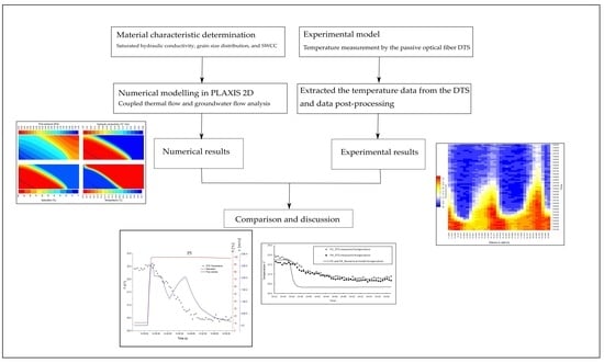
This work focuses on the monitoring of the seepage process in a laboratory scaled model by a passive DTS system. Most of the studies on this topic were performed by laboratory or field experiments. In this work, we combined a laboratory experiment with the numerical study for both thermal and groundwater flow. The study consists of the determination of material properties, a set-up of an experimental model of seepage while the optical fiber cable is embedded in the sand model and the numerical modeling of the seepage and heat flow in a geotechnical engineering software for two-dimensional finite element analysis (PLAXIS 2D). The experimental results from the physical model were compared with the numerical results obtained from the thermal and groundwater flow analysis. No optimization of material parameters was made, all the calculations were performed by using material parameters obtained from the laboratory tests and the related reference literature.
For the low temperature difference between the entered water and the soil, the active method was developed [15]. However, in this study, we showed the ability of the passive optical fiber DTS to monitor the seepage at the low temperature difference between the unsaturated sand and water in a laboratory scaled sand model.
2. Materials and Method
This study consists of the determination of material properties by the respective laboratory tests, an experimental model of seepage while the optical fiber cable is embedded in the sand model and the numerical modeling of the seepage and thermal flow in the PLAXIS 2D software.
2.1. Seepage and Heat Flow
The heat is transferred in soils by three mechanisms: conduction, convection, and radiation. In the thermometric analysis of seepage, the influence of the radiation process can be neglected because it affects only the surface layers of the soil due to its short day-night cycles duration [8]. A simplified equation based on energy conservation presents the heat transfer mechanism in the porous media which is shown in Equation (1) [21]. The second and third terms represent the heat transfer due to convection and conduction, respectively:
where is the bulk density of soil, is temperature, is the specific heat of the soil, is time, presents the water density (1000 kg/m3), is the specific heat of water (4181 J/kg/°C), is the specific discharge or Darcy velocity, and is the soil thermal conductivity.
Specific discharge is calculated using the continuity equation for mass conservation of water in porous media:
Considering constant , the equation for the volumetric water content , and Darcy’s law , Equation (2) leads to:
where is the hydraulic conductivity and depends on the saturation and porosity, and is the piezometric head.
Oftentimes, the Soil Water Characteristic Curve (SWCC) is used to describe the saturation - negative pore pressure (i.e., suction) relationship. We described the SWCC by the van Genuchten model [23] that relates the saturation to the pressure head :
where:
where is the saturation of the sand at the saturated condition usually equals to 1, is the residual saturation and , , and are empirical fitting parameters for the van Genuchten model. is related inversely to the air entry value (suction at which the soil begins to de-saturate). is the slope of SWCC once the air entry value has been exceeded [24] and is related to the curvature of the SWCC model in the high suction range. is usually fixed to in order to have an analytical solution for hydraulic conductivity. The hydraulic conductivity of material at the unsaturated condition () can be calculated using SWCC as seen from Equation (6) [23]:
where is hydraulic conductivity of saturated soil, is the fitting parameter (mostly 0.5).
The thermal conductivity of the soil ( and the heat capacity () as a function of soil saturation and porosity were estimated as [25]:
where , , and are the thermal conductivities of the particles, water (0.6 W/m/°C), and air (0.026 W/m/°C at normal laboratory conditions; 101.3 kPa, 20 °C) [26], respectively, is the particle density, and is the heat capacity of particles.
The heat flow boundaries are described by the Dirichlet and Neumann boundary condition types. In the Dirichlet type, a known temperature is prescribed on the boundary domain and time t [25,27]:
The Neumann type boundary condition for the heat transfer can be described by Equation (10):
where is the heat flux across the boundary and is the prescribed Neumann heat flux.
2.2. Soil
Silica dominated sand was used in this study. The material was purchased in 2019 from TERMIT d.d., a mining company that produces silica sand from the mines located in Moravče, Slovenia. We determined the saturated hydraulic conductivity, SWCC, dry and saturated densities, porosity, and the grain size distribution of the sand in the laboratory tests. The vendor provided the chemical composition of the sand [28]. The heat capacity and thermal conductivity of the sand particles were estimated from the literature based on the chemical composition of the material (1.36 W/m/°C [29], = 730 J/kg/°C [30]).
The chemical composition of the material, dry density , particle density , porosity , and coefficient of uniformity Cu are presented in Table 1.
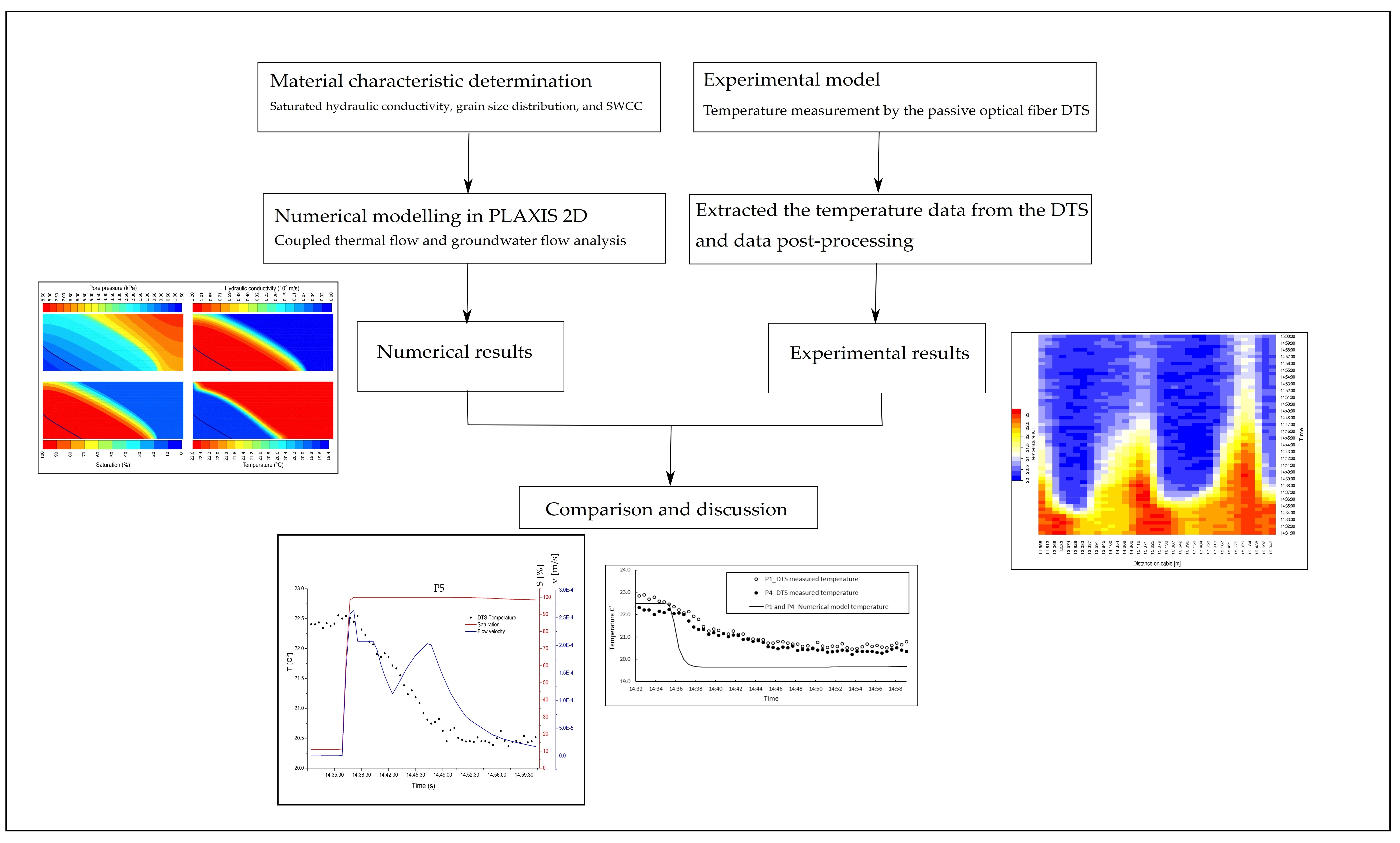
We determined the grain size distribution of the sand by the sieve analysis test, which is given in Figure 1.
SWCC was developed using the HYPROP evaporation method device (Meter group) [31,32] on a compacted sample. The sample was compacted to the same dry density as in the experimental model. With the HYPROP device, a continuous SWCC is obtained by simultaneously and continuously measuring suction with two high capacity tensiometers installed at different heights of the soil sample and weight change during drying. The typical range of the HYPROP device is from 0 to slightly above 100 kPa. When the suction difference between upper and lower tensiometer is greater than hydrostatic, the hydraulic conductivity as a function of saturation, could be measured for the unsaturated state. In the case of sand without fine particles (<0.063 mm), the volume change during the test is negligible and from the change in the mass of water the saturation could be calculated.
The saturated hydraulic conductivity, , was measured in constant head rigid wall permeameter using local total head measurements without saturation control (class 2 measurements). A permeameter with a diameter of 113 mm and a height of 405 mm was used. The sand was compacted to the same dry density as in the experimental sand model.
2.3. Experimental Model
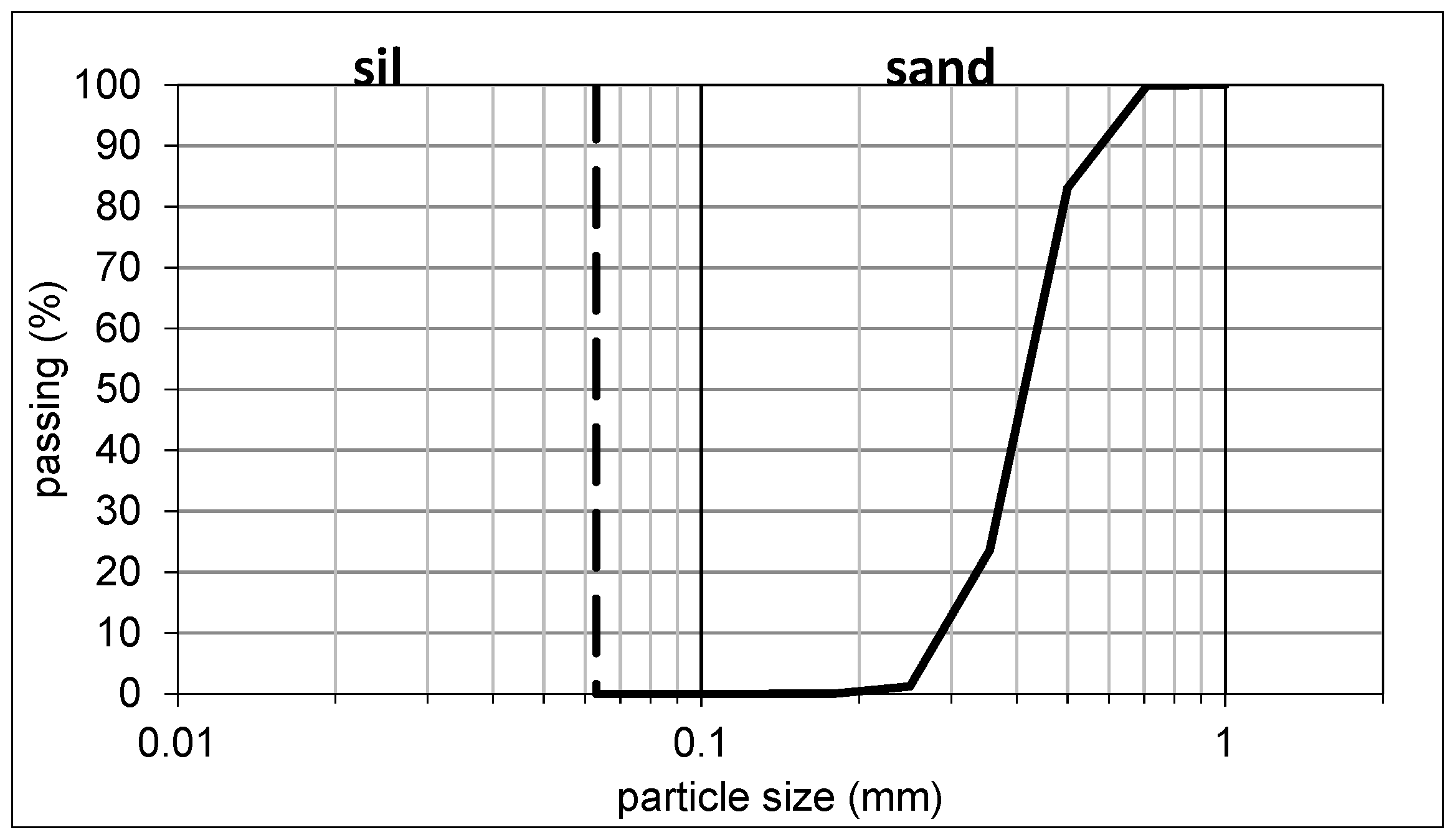
The physical model consisted of a rectangular box filled with sandy soil supported by wire mesh on the upstream and downstream faces and plexiglass at the sidewalls, with upstream and downstream tanks attached to it (Figure 2). Soil fill was 33.5 cm × 27 cm × 12 cm (length, width, height). The optical fiber cable was installed during soil placement. Homogeneous sand fill was assumed. It was anticipated that installed optical cables did not significantly influence the water and heat flow. Additionally, two thermometers were used to measure air and water temperature. The water level in the upper tank was controlled only by manual adjusting the position of a ball valve.
A passive optical fiber DTS system (SILIXA-XT-DTS) with 50/125 μm multi-mode optical fiber was used for the experiment. Optical fiber DTS employs the Optical Time Domain Reflectometry (OTDR) technique and uses characteristics of the Raman Spectroscopy of the light for temperature measurement. In this technique, DTS launches short pulses of light into the fiber optic cable and detects the Raman backscatter photons (Stokes and anti-Stokes) at regular time intervals by the fast photonic detector system [33,34]. The distance from the measurement point is determined by the runtime of the light, knowing its propagation velocity. The Raman scattering will be generated due to the transfer of energy between the launched laser photons and molecules of the material in optical fiber cable. The temperature in the vicinity of cable changes the energy state of molecules in the cable and influences the characteristics of Raman scattered photons. The Stokes intensity is irrelevant to the temperature, while the anti-Stokes intensity is highly dependent on the temperature. DTS measures the intensity of detected Raman scattered photons and use their ratio to obtain the temperature [35].
We performed the DTS measurement based on the duplexed single-ended configuration [36]. The distance between each temperature successive measurement (sampling interval) was selected as 10 inches (25.4 cm; the minimum allowable sampling interval for our system) to provide as many measuring points as possible in the model. The sampling time interval was 30 s. These intervals were appropriate to provide accurate and reliable measurements in our experiment. DTS temperature measurement is not fully independent for the adjacent sampling interval [37] and the abrupt change in temperature may be missed by the system. The distance between points reporting 10 to 90%, respectively, the true temperature changes at a step shift in temperature along the cable is called spatial resolution [38], which in our case was around 64 cm. In order to measure point temperature accurately, the length of the cable surrounds each measuring point (sensory ring) was increased to more than 50 cm by using two loops with the diameter of circa 8 cm. The loops were placed horizontally in the soil so the water flow was along the optical fiber cable. We made 12 measuring points by the cable loops as shown in Figure 2.
After the placement of the dry sand, the model was left in the laboratory for more than 48 h in order to equilibrate its temperature with the ambient temperature in the room (approximately 23 °C). Then, the measurement started to obtain the initial temperature of dry unsaturated sand. Filling of the upstream tank and seepage experiment started by opening the valve of the tap water. A PT100 thermometer was replaced in the upstream tank to measure the water temperature. The water temperature during the test was 19.6 ± 0.1 °C. The water level in the upstream tank was measured manually by measuring tape at given time intervals. After the maximum desired level at the upstream tank was reached the valve was closed. It was found that the volume of the upper tank was too small to maintain a nearly constant water level. As the water level dropped more than expected, due to the flow of water into the sand, the valve was temporarily opened again and after reaching the maximum desired level, the valve was closed (see Figure 6). At the downstream tank, the outflow gauge was opened for the free outflow from the tank. The water depth at the downstream tank corresponding to the steady-state flow was about 4 mm.
The DTS system is equipped with two PT100 thermometers. One of the thermometers was installed in the upstream tank to continuously measure the water temperature and the other one was used to measure the air temperature adjacent to the experimental model. The temperature measurement in our model was based on the internal calibration of the DTS system. A constant differential loss of light power equals to 0.255 dB/km was assigned for the system, as this was advised by the system guideline [39]. In the adjacent of the experimental model, a PT100 thermometer was placed to measure the ambient temperature. In this location, we placed 10 m of the cable as a reference section for the system to calibrate its measurements. SILIXA XT-DTS is calibrating its measurements using one or two reference sections where the PT100 thermometers are placed. In addition to that, the system calibrates the measurement using 200 m of the cable reference coil and a highly precise internal thermometer that existed inside the system. We calibrated the system and validated the DTS measurements by the internal calibration before the experiment, using two reference water baths containing hot and cold water with the constant temperatures.
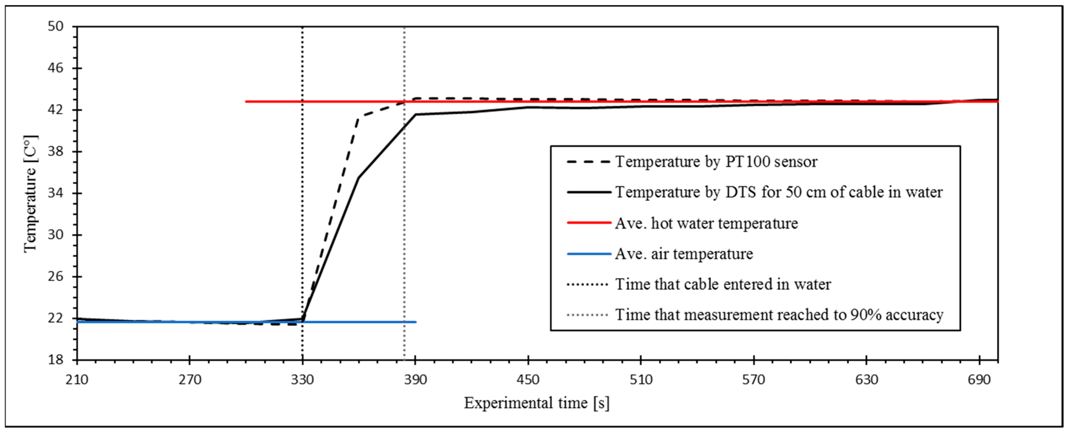
To describe the effect of the DTS system response time on the measurement of the step change in temperature, we conducted a separate experiment by embedding 50 cm of the cable together with a PT100 thermometer into an isolated hot water bath with a constant temperature of 43.8 °C. The result for the time response of the DTS system to reach 90% of the temperature change is shown in Figure 3.
2.4. Numerical Modeling
The numerical modeling of the seepage was performed in the geotechnical program PLAXIS 2D. PLAXIS 2D provides a continuous time-dependent analysis of groundwater and thermal flow in unsaturated media considering both conduction and convection in transient state. The soil is considered as homogeneous media and is not divided into different phases (local thermal equilibrium). The heat transfer due to vapor flow was neglected and heat transfer into the core of sand particles is not considered. Equations given in Section 2.1 are used by the PLAXIS for thermal and seepage analysis. The van Genucthen model (with parameters in Table 2) was used to describe the behavior of the sand at the unsaturated condition.
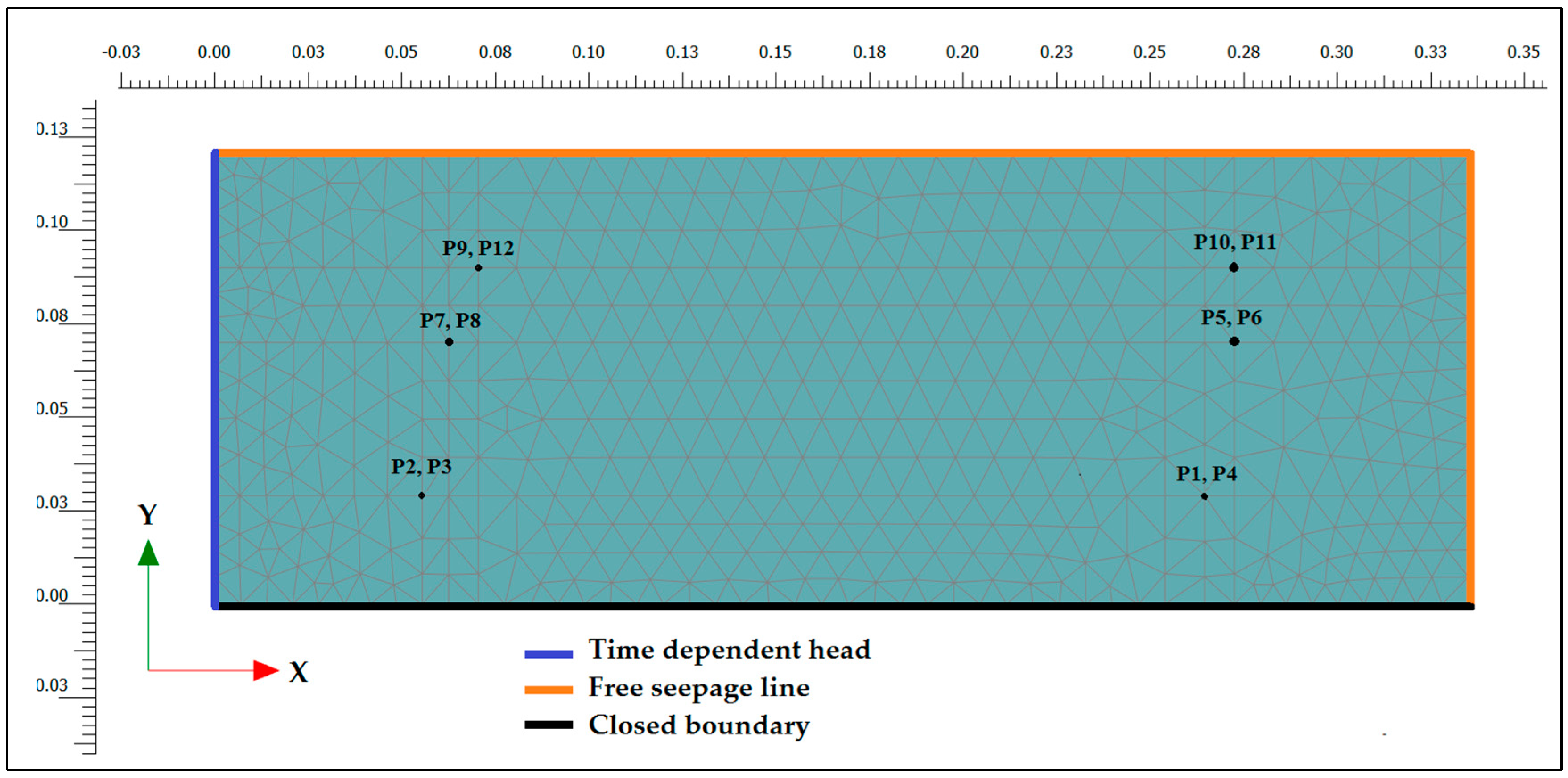
The numerical model was designed based on the material properties, the geometry of the experimental model, and the thermal and hydraulic boundary conditions of the experimental model. A coupled thermo-hydro analysis was performed using a two-dimensional (2D) numerical model consists of 913 15-nodes finite elements (Figure 4). Initially, the soil temperature was the same as measured before the seepage started and the sand was at residual saturation. The boundary conditions of the model with respect to the flow are presented in Figure 4. On the left, a time-dependent water head boundary has been assigned based on the experimental measurements (Figure 6). The top and right boundaries are seepage boundaries, which are closed boundaries until fully saturated when they start to allow outflow of water at pore pressure of 0 kPa (atmospheric pressure).
The boundary conditions in terms of temperature were defined as follows: at the upstream face, the Dirichlet boundary condition (see Equation (9)) was governed by the water temperature in the upstream tank, right and upper boundary had constant temperature equal to initial soil temperature, and at the bottom zero thermal flow was considered (see Neumann boundary condition, Equation (10)).
The first 30 min of the experimental model was simulated by the numerical model. The results of the calculations were saved every 30 s. The thermal conductivity, heat capacity, and hydraulic conductivity in each node were calculated continuously due to the change in saturation using Equations (4)–(8) based on the calculated pressure head by the PLAXIS 2D program.
3. Results
3.1. SWCC and Hydraulic Conductivity
The saturated hydraulic conductivity measured in constant head permeameter with local head measurements is given in Table 2. This table also presents the obtained parameters of the van Genuchten model for the best fit to the measured SWCC.
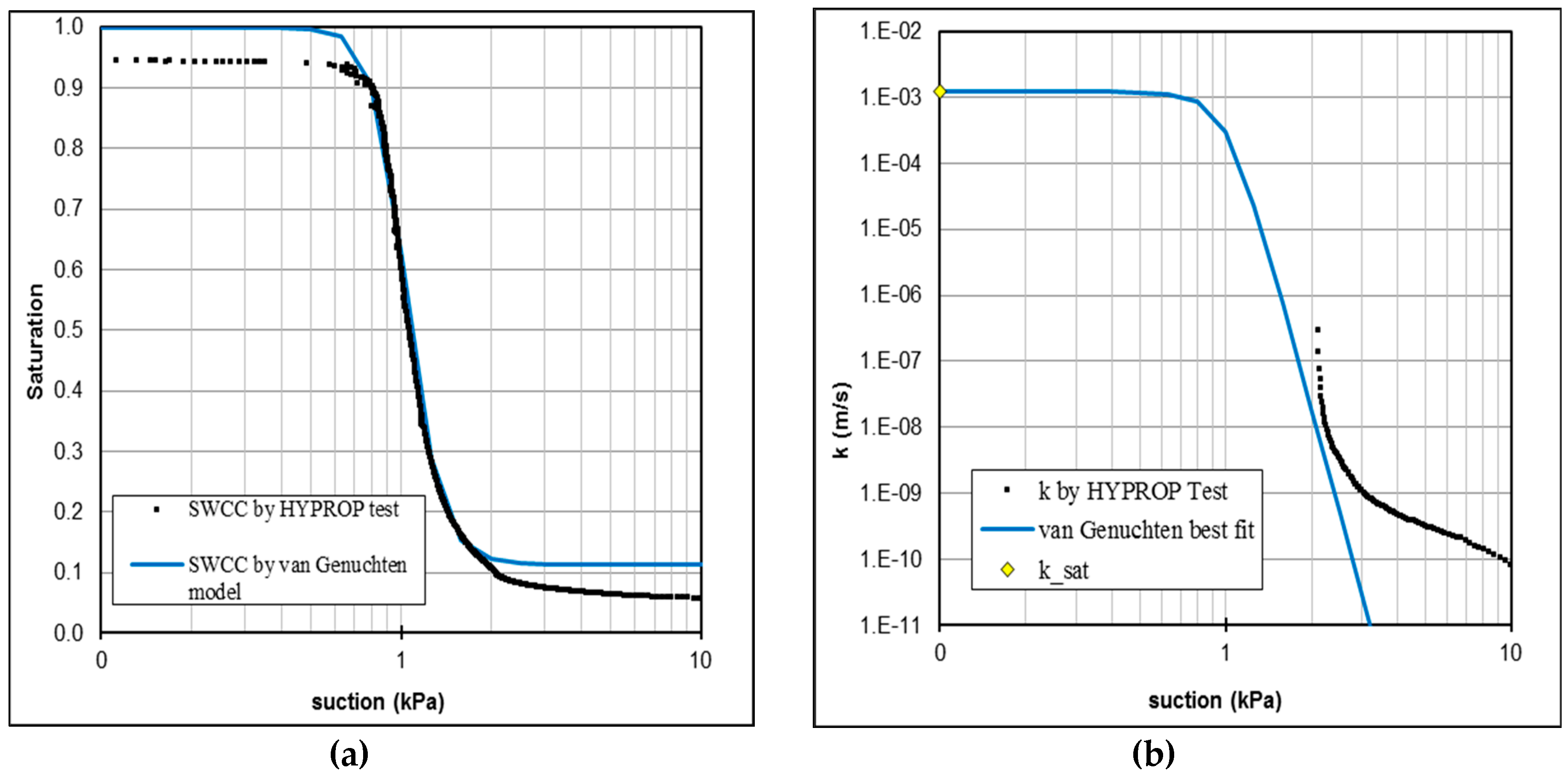
SWCC measured in the HYPROP device and the hydraulic conductivity as a function of suction are shown in Figure 5. The van Genuchten model for SWCC (blue lines in Figure 5) was fitted to the measured HYPROP data (Table 2) using the least-squares method in Excel spreadsheet. It was possible to measure unsaturated hydraulic conductivity by the evaporation method at the high suction end of SWCC. The van Genuchten model predicts hydraulic conductivity well to the suction (negative pore pressure) of 2.5 kPa. At greater suctions, the discrepancy between the measured and predicted hydraulic conductivity might be due to limitations of the evaporation method and probably does not represent true material behavior beyond the suction of 2.5 kPa.
3.2. Result of the Experimental Model
The recorded water levels at the upstream and downstream tanks are shown in Figure 6.
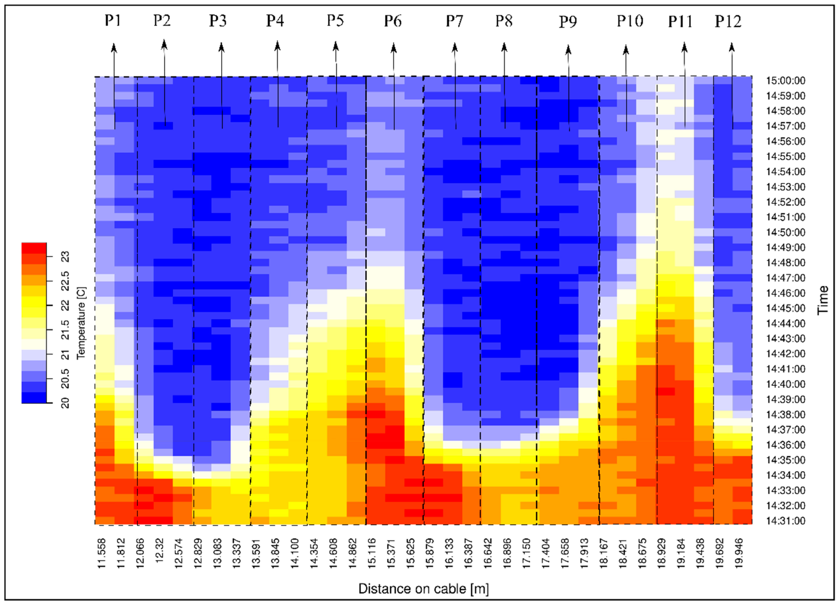
Figure 7 presents the measured temperature by the optical fiber cable embedded in the soil before and during the experiment. The length of the cable corresponded to each measuring point is marked in Figure 7 by the dashed line.
The measured temperature during the first two minutes presents the soil temperature when the water flow was not yet started. Almost a homogenous temperature distribution is observed before the seepage flow into the model was taken place. The water inflow into the upstream tank was started at 14:34:00. Points 2 and 3 are located near the upstream tank and the temperature decrease in these points is evident at the first reported time after the start of filling the upstream tank. It is clear from the measured temperature that points 7, 8, 9, and 12 are experiencing the temperature decline respectively after points 2 and 3. All these points are located at the upstream zone of the model and with increasing the water level the seepage flow is propagating towards these locations. The temperature results show that each pair of symmetrically located points with respect to the model vertical central plane (e.g., P1 and P4 in Figure 2) provide similar temperature variation during the experiment.
With the propagation of the seepage through the model, the temperature decreases in the soil towards the downstream side. A time difference related to the temperature drop in consecutive measuring points can be used for the estimation of seepage propagation in the model. This estimation assumes thermal retardation to be negligible. With continuing the seepage flow the temperature in all seepage zone tends to be stable.
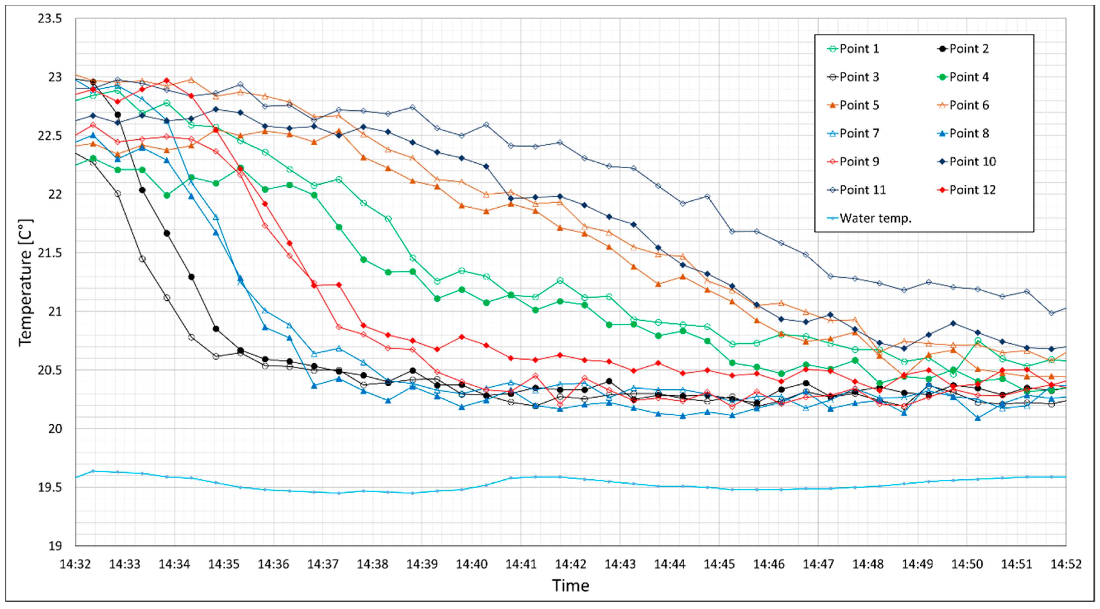
Figure 8 demonstrates the temperature variation during the experiment for all measuring points.
3.3. Result of Numerical Modeling
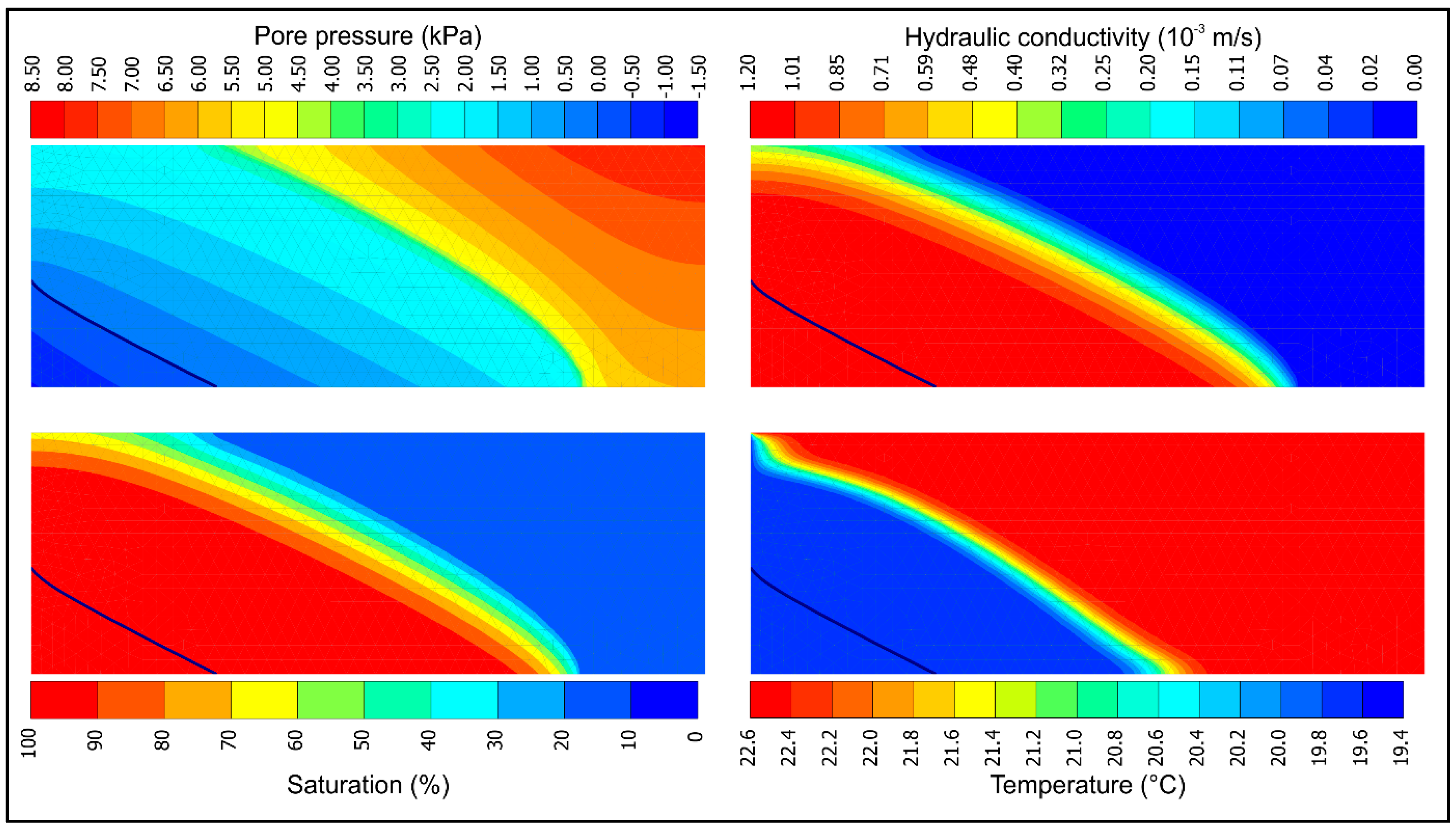
The results from the numerical modeling for pore pressure, hydraulic conductivity, saturation, and temperature variation at the simulation time of 120 s are presented in Figure 9.
The bold line in Figure 9 presents the phreatic line. It can be seen that the saturation front precedes the heat flow in the sand model. Larger values for hydraulic conductivity and saturation were obtained when the pore pressure (negative in PLAXIS) increases.
4. Discussion and Comparison
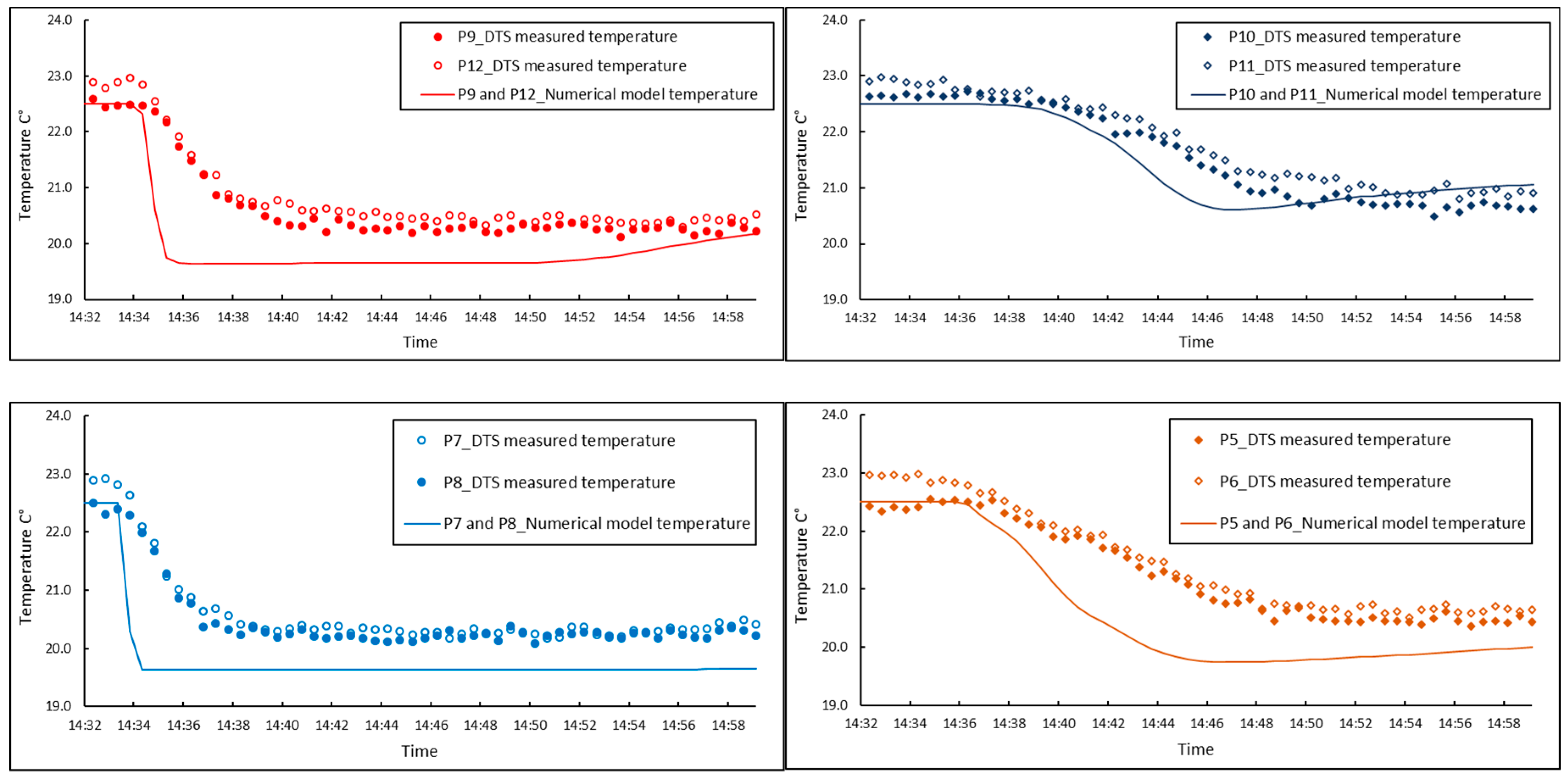
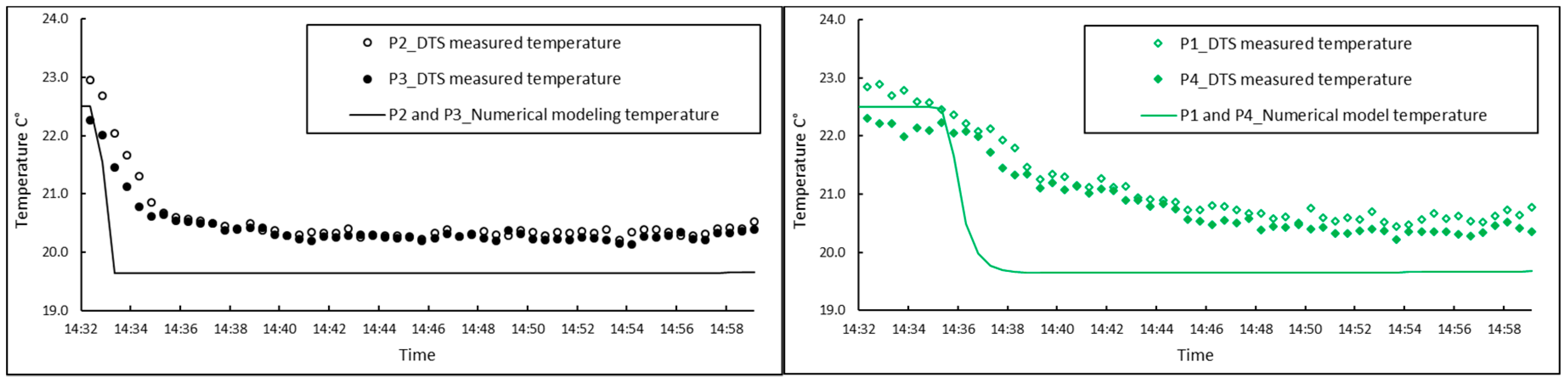
The temperature variations for 12 measuring points were compared to the results from numerical modeling (Figure 10).
A short time gap can be observed between the temperature drop in the numerically modeled and measured temperatures. This is mostly due to the response time of the DTS system (about 60 s, see Figure 3) to fast changes of temperature. This shows that the response time has a significant role in the heat measurement by the DTS system in a small-scale experimental model with fast seepage. However, for the long-term temperature monitoring in real size structures, this effect can be negligible. The response time of the DTS system also attributed to the gradual change in the measured temperature in the sand model. The temperature gradient is higher for the points that are in the upstream zone. This phenomenon will be described by looking at the results from the seepage flow velocity in Figure 11. The temperature gap between the DTS measurements and numerical results (Figure 10) can be partially described by the accuracy of the DTS measurement. The accuracy of point-mode measurements also depends on the size of the sensory ring (inner diameter of the ring) and the length of optical fiber in the sensory ring [40]. Studies show that the ideal size and length of the sensory ring also depend on the type and external diameter of the optical fiber [40,41]. The inner diameter of the sensory ring should be kept in a range to measure specifically the one-year point and to avoid the adverse effects of optical fiber bending. A ring with a smaller diameter than the critical value can cause step losses in the optical fiber, which must be corrected with further manual calibration techniques [42,43].
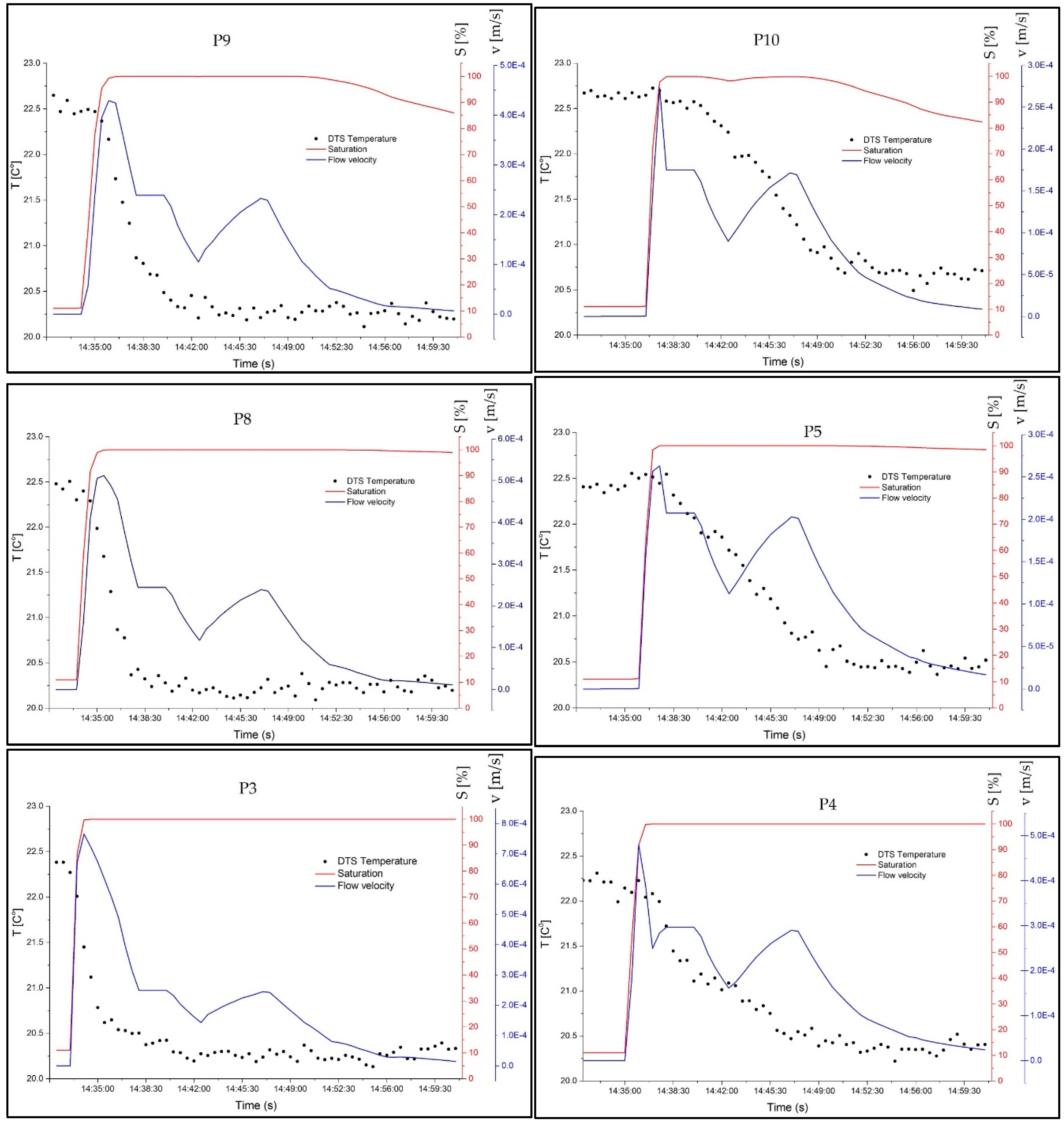
The other factor that was studied is the relationship between the degree of saturation and seepage flow velocity with the measured temperature by DTS. Figure 11 presents the numerical results for the degree of saturation, the flow velocity, and the measured temperature variation during the experiment. The results demonstrated in Figure 11 present the ability of temperature monitoring for detecting the seepage presence. With increasing the water content in the sand, the temperature is decreasing. The results show that saturation can be monitored in the early phases by temperature measurement. The temperature reduction is started by increasing the degree of saturation in the sand. The average seepage velocity may be estimated using the time gap between the start of temperature drop in various zones of the sand model. It is evident from the results in Figure 11 that this time gap approximately represents the time between the seepage propagation in the selected measured points of the model.
The amount of heat transfer by the advection process directly depends on the average velocity of seepage, as can be seen in Equation (1). The results in Figure 11 show the strong dependency of temperature variation on the magnitude of the flow velocity. For the points which are located at the upstream boundary, the seepage flow velocity is increased dramatically high. Due to this effect, the temperature values in these points are decreasing with a high gradient. On the other hand, for the points at the downstream side, the flow velocity is increased less and causes a gradual temperature variation. Higher flow velocity increases the gradient of temperature reduction graph in the sand and a low flow velocity causes a gradual temperature decreasing in the model.
The temperature changes occur by the increase in the degree of saturation. This is due to changes in the thermal conductivity of the porous media. However, when the seepage flow propagates into the sand, the temperature variation is due to the convection process, which is directly proportional to the flow velocity. In this case, the temperature is decreasing faster.
In this experiment, the water seepage observed to flow out of the sand model at 14:39:00. For Point 10, which is located at the upper layer of downstream, there is not any clear temperature reduction at this time. It means that seepage detection by visual observation was faster than the temperature monitoring in Point 10 for this experimental model. For real scale structures, it is economic to perform a seepage analysis and install the optical fiber based on the magnitude of leakage risk. This will decrease the monitoring system cost and increase the ability of the system for early seepage detection.
5. Conclusions
This study presents seepage detection by the passive optical fiber DTS system in a laboratory-scale model. Numerical modeling for the seepage and the heat transfer in the sand was performed. The effect of suction (negative pore pressures) in seepage behavior for such a small model was clearly high; however, for a real size structure, this effect might be not important. The results from both experimental and numerical modeling lead to the flowing conclusions:
- The passive optical fiber DTS system that measures the natural temperature of media was capable to detect the seepage propagation in the sand.
- The seepage is detectable in the sand by the accurate temperature measurement even with the small difference between the temperature of the reservoir water and the soil (about 3 degrees).
- A very clear relationship between the increase of the degree of saturation and temperature declination was observed in the results.
- The numerical model describes temperature measurements reasonably well.
- A short time gap between seepage propagation and its detection by DTS is observed. This gap is due to averaging of the temperature in each measurement length and the system response time (see Figure 3)
- The temperature reduction in the seepage zone strongly depends on the seepage average velocity and not necessarily on the degree of saturation.
- In the numerical calculation, it was observed that saturation preceded the heat flow.
- The numerical analysis of seepage should be considered before the installation of the optical fiber cable for the passive DTS system. Increasing the cable length for the zones with higher seepage risk will increase the chance for its early detection. However, the length of the cable in the zones with lower risk can be decreased.
- The distribution of the cable in the structure should be precisely recorded. A wrong recorded location may lead to the wrong localization of the seepage.
Author Contributions
Y.G. designed the experiment, did the numerical analysis and experiment measurement and prepared and edited the manuscript. M.M. did the HYPROB test, participated in the material properties determination, performed the numerical modeling, and reviewed the manuscript. A.V. participated in the DTS software and measurement, setting the instrument, and gave suggestions for the measurement process. J.Ř., and A.K. provided the resources for the experiment, supervised the study, and reviewed the manuscript. All authors have read and agreed to the published version of the manuscript.
Funding
This research received funds from the Slovenian Research Agency (research core funding No. P2-0180).
Acknowledgments
We appreciate the anonymous reviewers for their valuable comments and efforts to improve this manuscript. We would like to thank Gašper Rak for his valuable cooperation. The authors also acknowledge the financial support from the Slovenian Research Agency and contribution from the project FAST-S-19-5714 (Probability assessment of internal instability in earth structures and in hydraulic structures, BUT Brno, Czech Republic).
Conflicts of Interest
The authors declare no conflict of interest.
References
- Torres, R.L. Considerations for Detection of Internal Erosion in Embankment Dams. In Proceedings of the Biennial Geotechnical Seminar Conference, Denver, CO, USA, 7 November 2008; ASCE: Reston, VA, USA; pp. 82–98. [Google Scholar] [CrossRef]
- Bonelli, S.; Courivaud, J.-R.; Fry, J.-J. Internal erosion on dams and dikes: Lessons from experience and modelling. In Proceedings of the 24th ICOLD Congres, Kyoto, Japan, 6 June 2012; ICOLD: Kyoto, Japan; pp. 366–388. [Google Scholar]
- ICOLD Internal Erosion of Existing Dams, Levees and Dikes, and Their Foundations; ICOLD Bulletin 164; ICOLD: Paris, France, 2017; Volume 1.
- Su, H.; Yang, M.; Wen, Z. Multi-Layer Multi-Index Comprehensive Evaluation for Dike Safety. Water Resour. Manag. 2015, 29, 4683–4699. [Google Scholar] [CrossRef]
- Foster, M.; Fell, R.; Spannagle, M. The statistics of embankment dam failures and accidents. Can. Geotech. J. 2000, 37, 1000–1024. [Google Scholar] [CrossRef]
- Novak, P.; Moffat, A.I.B.; Nalluri, C.; Narayanan, R. Hydraulic Structures, 4th ed.; Taylor & Francis: New York, NY, USA, 2007; ISBN 9780415386258. [Google Scholar]
- Kappelmeyer, O. The use of near surface temperature measurements for discovering anomaliers due to causes at depths. Geophys. Prospect. 1957, 5, 239–258. [Google Scholar] [CrossRef]
- Johansson, S. Seepage Monitoring in Embankment Dams. Doctoral Thesis, Royal Institute of Technology, Stockholm, Sweden, 1997. [Google Scholar]
- Dornstadter, J. Detection of internal erosion in embankment dams. In Proceedings of the Nineteenth ICOLD Congress, Florence, Italy, 19–31 May 1997; ICOLD: Paris, France; pp. 87–102. [Google Scholar]
- Ukil, A.; Braendle, H.; Krippner, P. Distributed temperature sensing: Review of technology and applications. IEEE Sens. J. 2012, 12, 885–892. [Google Scholar] [CrossRef] [Green Version]
- Aufleger, M.; Dornstädter, J.; Huber, K.; Strobl, T. Sensitive Long-Term-Monitoring of Embankment Dams by Fibre Optic Temperature Laser Radar: First Results. In ICOLD XIX; ICOLD: Florence, Italy, 1997; pp. 443–446. [Google Scholar]
- Orrell, P.R. Distributed Fibre Optic Temperature Sensing. Sens. Rev. 1992, 12, 27–31. [Google Scholar] [CrossRef]
- Johansson, S.; Sjodahl, P. Seepage Measurements and Internal Erosion Detection using the Passive Temperature Method. In Assessment of the Risk of Internal Erosion of Water Retaining Structures: Dams, Dykes and Levees; Technische Universität München: Munich, Germany, 2007; pp. 186–192. ISBN 978-3-940476-04-3. [Google Scholar]
- Čejka, F.; Beneš, V.; Glac, F.; Boukalová, Z. Monitoring of seepages in earthen dams and levees. Int. J. Environ. Impacts 2018, 1, 267–278. [Google Scholar] [CrossRef]
- Perzlmaier, S.; Aufleger, M.; Dornstädter, J. Detection of Internal Erosion by Means of the Active Temperature Method. In Assessment of the Risk of Internal Erosion of Water Retaining Structures: Dams, Dykes and Levees; Technische Universität München: Munich, Germany, 2007; ISBN 978-3-940476-04-3. [Google Scholar]
- Su, H.; Kang, Y. Design of System for Monitoring Seepage of Levee Engineering Based on Distributed Optical Fiber Sensing Technology. Int. J. Distrib. Sens. Networks 2013, 10. [Google Scholar] [CrossRef]
- Su, H.; Tian, S.; Kang, Y.; Xie, W.; Chen, J. Monitoring water seepage velocity in dikes using distributed optical fiber temperature sensors. Autom. Constr. 2017, 76, 71–84. [Google Scholar] [CrossRef]
- Yosef, T.Y.; Song, C.R.; Chang, K.T. Hydro-thermal coupled analysis for health monitoring of embankment dams. Acta Geotech. 2017, 13, 447–455. [Google Scholar] [CrossRef]
- Radzicki, K.; Bonelli, S. Thermal Seepage Monitoring in the Earth Dams with Impulse Response Function Analysis Model. In Proceedings of the 8th ICOLD European Club Symposium, Innsbruck, Austria, 22–23 September 2010; pp. 624–629. [Google Scholar]
- Khan, A.A.; Vrabie, V.; Mars, J.I.; Girard, A.; D’Urso, G. A source separation technique for processing of thermometric data from fiber-optic DTS measurements for water leakage identification in dikes. IEEE Sens. J. 2008, 8, 1118–1129. [Google Scholar] [CrossRef] [Green Version]
- Nield, D.A.; Bejan, A. Convection in Porous Media; Springer: New York, NY, USA, 2006; ISBN 0-387-29096-6. [Google Scholar]
- Diao, N.; Li, Q.; Fang, Z. Heat transfer in ground heat exchangers with groundwater advection. Int. J. Therm. Sci. 2004, 43, 1203–1211. [Google Scholar] [CrossRef]
- van Genuchten, M.T. A Closed-form Equation for Predicting the Hydraulic Conductivity of Unsaturated Soils. Soil Sci. Soc. Am. J. 1980. [Google Scholar] [CrossRef] [Green Version]
- Benson, B.C.H.; Chiang, I.; Chalermyanont, T.; Sawangsuriya, A. Estimating van Genuchten Parameters α and n for Clean Sands from Particle Size Distribution Data. In Proceedings of the Geo-Congress, Atlanta, GA, USA, 23–26 February 2014; ASCE: Reston, VA, USA. [Google Scholar] [CrossRef]
- Brinkgreve, R.B.J.; Kumarswamy, S.; Haxaire, A. Thermal and coupled THM analysis; Plaxis bv: DELFT, Netherlands, 2017. [Google Scholar]
- Stephan, K.; Laesecke, A. The Thermal Conductivity of Fluid Air. J. Phys. Chem. Ref. Data 1985, 14, 227–234. [Google Scholar] [CrossRef] [Green Version]
- Diersch, H.-J.G. FEFLOW: Finite Element Modeling of Flow, Mass and Heat Transport in Porous and Fractured Media; Springer: Heidelberg, Germany, 2014; ISBN 978-3-642-38738-8. [Google Scholar]
- Termit Catalog for Quartz and ceramic coated sands. Available online: https://www.termit.si/en/wp-content/uploads/sites/3/2018/08/kremenov_pesek.pdf. (accessed on 25 September 2019).
- Kiyohashi, H.; Sasaki, S.; Masuda, H. Effective thermal conductivity of silica sand as a filling material for crevices around radioactive-waste canisters. High Temp. High Press. 2003, 35/36, 179–192. [Google Scholar] [CrossRef]
- Hemingway, B.S. Quartz; heat capacities from 340 to 1000 K and revised values for the thermodynamic properties. Am. Mineral. 1987, 72, 273–279. [Google Scholar]
- Schindler, U.; Müller, L. Soil hydraulic functions of international soils measured with the Extended Evaporation Method (EEM) and the HYPROP device. Open Data J. Agric. Res. 2017, 3, 10–16. [Google Scholar] [CrossRef] [Green Version]
- UMSP. Manual HYPROP, Version 2015-01; UMS GmbH: Munich, Germany, 2015. [Google Scholar]
- Hartog, A.H.; Gold, M.P.; Leach, A.P. Optical Time-Domain Reflectometry. United States Patent No. 4823166, 18 April 1989. [Google Scholar]
- Odic, R.M.; Jones, R.I.; Tatam, R.P. Distributed Temperature Sensor for Aeronautic Applications. In Proceedings of the 15th Optical Fiber Sensors Conference, Portland, OR, USA, 6–10 May 2002; IEEE: Piscataway, NJ, USA; pp. 459–562. [Google Scholar] [CrossRef]
- Long, D.A. Raman spectroscopy; McGraw-Hill International: New York, NY, USA, 1977; ISBN 0070386757. [Google Scholar]
- Hausner, M.B.; Suárez, F.; Glander, K.E.; van de Giesen, N. Calibrating Single-Ended Fiber-Optic Raman Spectra Distributed Temperature Sensing Data. Sensors 2011, 11, 10859–10879. [Google Scholar] [CrossRef]
- Selker, J.S.; Tyler, S.; van de Giesen, N. Comment on ‘“Capabilities and limitations of tracing spatial temperature patterns by fiber-optic distributed temperature sensing”’ by Liliana Rose et al. Water Resour. Res. 2014, 50, 5372–5374. [Google Scholar] [CrossRef] [Green Version]
- Tyler, S.W.; Selker, J.S.; Hausner, M.B.; Hatch, C.E.; Torgersen, T.; Thodal, C.E.; Schladow, S.G. Environmental temperature sensing using Raman spectra DTS fiber-optic methods. Water Resour. Res. 2009, 45, 11. [Google Scholar] [CrossRef] [Green Version]
- Silixa Ltd. SILIXA XT-DTS Software Manual; Silixa House Elstree: Borehamwood, UK, 2014. [Google Scholar]
- Koudelka, P.; Latal, J.; Vitasek, J.; Hurta, J.; Siska, P.; Liner, A.; Papes, M. Implementation of optical meanders of the optical- fiber DTS system based on Raman stimulated scattering into the building processes. Adv. Electr. Electron. Eng. 2012, 2, 187–194. [Google Scholar] [CrossRef]
- Koudelka, P.; Liner, A.; Papes, M.; Latal, J.; Vasinek, V.; Hurta, J.; Vinkler, T.; Siska, P. New sophisticated analysis method of crystallizer temperature profile utilizing optical fiber DTS based on the stimulated Raman scattering. Adv. Electr. Electron. Eng. 2012, 10, 106–114. [Google Scholar] [CrossRef]
- Hausner, M.B.; Kobs, S. Identifying and Correcting Step Losses in Single-Ended Fiber-Optic Distributed Temperature Sensing Data. J. Sensors 2016. [Google Scholar] [CrossRef] [Green Version]
- Mcdaniel, A.; Tinjum, J.M.; Hart, D.J.; Fratta, D. Temperature Sensing Networks. IEEE Sens. J. 2018, 18, 2342–2352. [Google Scholar] [CrossRef]
Figure 1.
The grain size distribution curve.

Figure 2.
Geometry of the experimental model. (a) Side view of the model; (b) top view of the model at the elevation of 2.9 cm.
Figure 2.
Geometry of the experimental model. (a) Side view of the model; (b) top view of the model at the elevation of 2.9 cm.

Figure 3.
Response time of the system. The temperature measurement by the DTS reached to 90% of the temperature shift at the second reported temperature (60 s after cable entered in the hot water).
Figure 3.
Response time of the system. The temperature measurement by the DTS reached to 90% of the temperature shift at the second reported temperature (60 s after cable entered in the hot water).

Figure 4.
Discretization of the model into finite elements in the PLAXIS 2D software and definition of boundary condition with respect to the flow condition.
Figure 4.
Discretization of the model into finite elements in the PLAXIS 2D software and definition of boundary condition with respect to the flow condition.

Figure 5.
(a) Soil Water Characteristics Curve (SWCC). Results for both the HYPROP device test and the van Genuchten approximation are presented; (b) relative hydraulic conductivity curve.
Figure 5.
(a) Soil Water Characteristics Curve (SWCC). Results for both the HYPROP device test and the van Genuchten approximation are presented; (b) relative hydraulic conductivity curve.

Figure 6.
Time dependency of water level at upstream and downstream tanks (left and right boundaries).
Figure 6.
Time dependency of water level at upstream and downstream tanks (left and right boundaries).

Figure 7.
Temperature measured by the optical fiber Distributed Temperature Sensor (DTS) before and during the experiment.
Figure 7.
Temperature measured by the optical fiber Distributed Temperature Sensor (DTS) before and during the experiment.

Figure 8.
Temperature variation for measuring points.

Figure 9.
Schematic results from numerical modeling in PLAXIS 2D at running time 120 s. Note that compression (pore pressure) is negative in PLAXIS.
Figure 9.
Schematic results from numerical modeling in PLAXIS 2D at running time 120 s. Note that compression (pore pressure) is negative in PLAXIS.

Figure 10.
Measured temperature by the optical fiber DTS and the calculated temperature by the numerical modeling. The results are presented for all 12 measuring points. Points are located in figures based on their location at the experimental model.
Figure 10.
Measured temperature by the optical fiber DTS and the calculated temperature by the numerical modeling. The results are presented for all 12 measuring points. Points are located in figures based on their location at the experimental model.


Figure 11.
Measured temperature by optical fiber DTS, the calculated degree of saturation and flow velocity by the numerical modeling. The results are shown for six measuring points at three different elevations.
Figure 11.
Measured temperature by optical fiber DTS, the calculated degree of saturation and flow velocity by the numerical modeling. The results are shown for six measuring points at three different elevations.


Table 1.
The material characteristics.
| Chemical Composition | Sand Properties | |||||||
|---|---|---|---|---|---|---|---|---|
| % SiO2 | % Fe2O3 | % Al2O3 | % TiO2 | % K2O | Cu | |||
| 99.17 | 0.120 | 0.348 | 0.071 | 0.097 | 2.7 | 1.54 | 0.435 | 1.52 |
Table 2.
Obtained parameters for the van Genuchten approximation for best fit to the results of the test by the evaporation method (HYPROP device) and the measured saturated hydraulic conductivity of the sand.
Table 2.
Obtained parameters for the van Genuchten approximation for best fit to the results of the test by the evaporation method (HYPROP device) and the measured saturated hydraulic conductivity of the sand.
| (m/s) | ||||||
|---|---|---|---|---|---|---|
| 1 | 0.11 | 9.70 | 8.06 | 0.876 | 0.00 | 1.23 × 10⁻³ |
© 2020 by the authors. Licensee MDPI, Basel, Switzerland. This article is an open access article distributed under the terms and conditions of the Creative Commons Attribution (CC BY) license (http://creativecommons.org/licenses/by/4.0/).
Share and Cite
MDPI and ACS Style
Ghafoori, Y.; Maček, M.; Vidmar, A.; Říha, J.; Kryžanowski, A. Analysis of Seepage in a Laboratory Scaled Model Using Passive Optical Fiber Distributed Temperature Sensor. Water 2020, 12, 367. https://doi.org/10.3390/w12020367
AMA Style
Ghafoori Y, Maček M, Vidmar A, Říha J, Kryžanowski A. Analysis of Seepage in a Laboratory Scaled Model Using Passive Optical Fiber Distributed Temperature Sensor. Water. 2020; 12(2):367. https://doi.org/10.3390/w12020367
Chicago/Turabian StyleGhafoori, Yaser, Matej Maček, Andrej Vidmar, Jaromír Říha, and Andrej Kryžanowski. 2020. "Analysis of Seepage in a Laboratory Scaled Model Using Passive Optical Fiber Distributed Temperature Sensor" Water 12, no. 2: 367. https://doi.org/10.3390/w12020367
Note that from the first issue of 2016, this journal uses article numbers instead of page numbers. See further details here.