A Study of Precipitation Patterns through Stochastic Ordering


1
School of Statistics, University of International Business and Economics, Beijing 100029, China
2
Department of Statistics, Purdue University, West Lafayette, IN 47807, USA
*
Author to whom correspondence should be addressed.
Water 2020, 12(2), 351; https://doi.org/10.3390/w12020351
Submission received: 21 December 2019
/
Revised: 20 January 2020
/
Accepted: 22 January 2020
/
Published: 27 January 2020
(This article belongs to the Special Issue Application of Space-Time Statistics in Water Resources)
Abstract
:The study of spatial and temporal changes in precipitation patterns is important to agriculture and natural ecosystems. These changes can be described by some climate change indices. Because these indices often have skewed probability distributions, some common statistical procedures become either inappropriate or less powerful when they are applied to the indices. A nonparametric approach based on stochastic ordering is proposed, which does not make any assumption on the shape of the distribution. This approach is applied to the average length of the period between two adjacent precipitation days, which is called the average number of consecutive dry days (ACDD). This approach is shown to be able to reveal some patterns in precipitation that other approaches do not. Using daily precipitations at 756 stations in China from 1960 to 2015, this work compares the ACDDs in three periods, 1960–1965, 1985–1990, and 2010–2015 for each province in China. The results show that ACDD increases stochastically from the period 1960–1965 to either the period 1985–1990 or the period 2010–2015, or from the period 1985–1990 to the period 2010–2015 in all but three provinces in China.
1. Introduction
Extreme precipitation events have large impacts on agriculture and natural ecosystems [1,2]. They have tended to occur more frequently in recent years [3] with the increased risk of droughts, floods, and agricultural and natural disasters. The understanding of the spatial and temporal patterns of precipitation change is very important to a country, such as China, where the available water per person is only one-third of the world average [4]. Spatial and temporal changes in precipitation have been studied for different regions in China, for example, Southwestern China [5], Northwestern China [6], the Yangtze River Delta [7], the Zhujiang River Basin [8], and other specific regions [9,10,11,12,13,14,15,16]. These results agree with the literature in that the observed changes in precipitation extremes are much less spatially coherent and statistically significant compared to observed changes in temperature extremes [17,18].
To describe and understand the various aspects of climate changes, climate change indices have been developed, and some of the indices concern climate extremes [19]. For precipitation, consecutive dry days (CDD) has been employed as one of the measures of extreme precipitation and adapted by many researchers [1,14,16,20,21,22,23,24,25,26,27,28,29]. It is defined as the maximum number of consecutive dry days with precipitation less than a certain threshold during a certain period of time where both the threshold and the period may vary [30]. The period could be a calendar year [8] or cold season or warm season [31].
Many scholars have used CDD as one of the climate change indices in the study of spatiotemporal patterns of precipitation in China. One common question in these studies is whether the CDD exhibits a monotonic (i.e., increasing or decreasing) or linear trend. The presence of such a trend represents a change in precipitation pattern. The question is answered primarily in three ways, visualization [29,32], the Mann–Kendall (MK) trend test [7,20,26,33,34,35,36], and the linear regression model [37,38,39]. The MK test finds no significant trend in the majority of stations across the country [20,33] or in some specific region [34] while the regression model reveals positive trends at 46% of the stations in Northeast China [37], a significant decreasing trend in Northwest China [38], and no significant trend in the Hengduan Mountains region [39]. This agrees with the findings in [17,18] that the observed changes in precipitation extremes are statistically less significant compared to observed changes in temperature extremes.
From a statistical point of view, more powerful statistical procedures that could detect changes the current methods do not would be helpful. We propose a new statistical approach to the study of changes in precipitation that has a higher power than the existing test procedures. The key idea involves stochastic ordering [40] that has been used in survival analysis [41] and operations research [42]. One random variable is stochastically larger than another random variable if its cumulative distribution function is less than or equal to that of another variable. Formal statistical tests have been developed for stochastic ordering that can be applied to compare the climate indices in different periods. We pick three periods, 1960–1965, 1985–1990, and 2010–2015, and make a pairwise comparison of the mean length of consecutive dry days in these three periods by applying a formal nonparametric statistical test.
2. Materials and Methods
2.1. Study Area and Data
China is located in East Asia, to the west of the Pacific Ocean, with a total area of 9.6 million km2 approximately (the 3rd largest in the world). Its elevation ranges from −154.31m (Aydingkol Lake) to 8844.43m (Mount Qomolangma). Eleven of the seventeen tallest mountain peaks on Earth are located on China’s western borders, among which the Himalayas is the world’s tallest, spreading over the border between China, India, Nepal, Bhutan, and Pakistan. From these heights in the west, the land descends in steps like a terrace. China has numerous rivers, with the Yangtze River being the longest in China (the 3rd longest in the world) and the Yellow River being the 2nd longest.
Annual precipitation in China, in general, decreases from the southeast coast to the northwest inland, with a vast difference between some regions. Most regions have more precipitation in summer and fall than in winter and spring. In 2017, the average annual precipitation in China equaled 641.3mm, which represents a 12% decrease from 2016. There is a fluctuation of average precipitation from year to year in China.
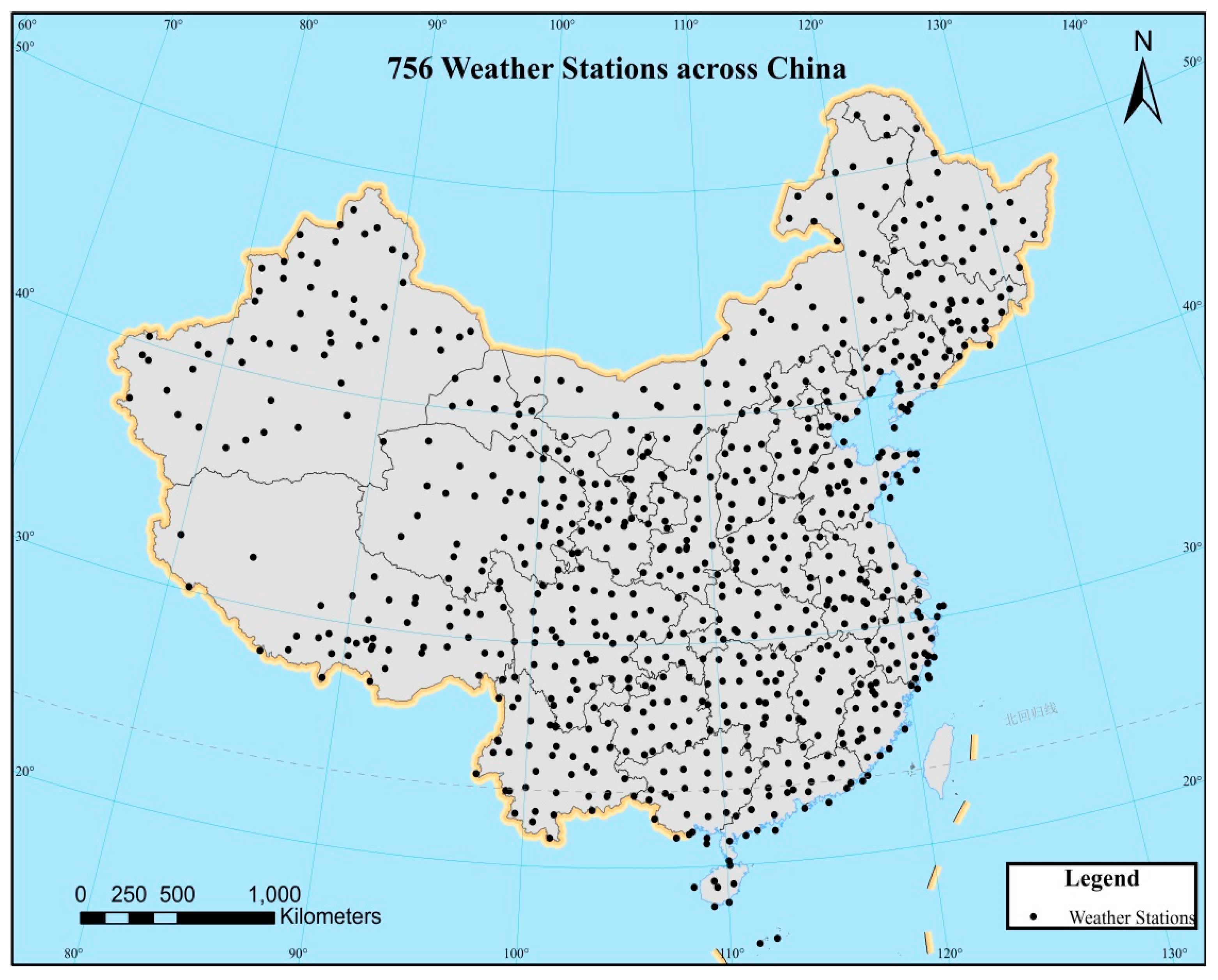
We obtained daily precipitation data at 756 national key weather stations across China from 1960 to 2015 from the China Meteorological Administration. Figure 1 shows the locations of these stations, which are unevenly distributed over China, with the sampling density decreasing from the southeast coast to the northwest inland. Data at these stations are carefully validated before they are released to the public. Potential errors or outliers are addressed in the validation process. However, there are missing values at some stations. Some of the missing values are a result of the retirement or addition of some stations. Among all 756 stations, 569 have complete precipitation data.
2.2. Maximum Number and the Average of Consecutive Dry Days
The maximum number of consecutive dry days (CDD) was first defined as the maximum number of consecutive days with precipitation less than 1 mm [30] in a calendar year. For areas with relatively low precipitation (e.g., Northwest China), the threshold can be lowered. For example, considering the vast regional differences in China, a threshold of 0.1 mm/day was used in [31], where the maximum of consecutive dry days was obtained for the warm season and the cold season. It is an index for assessing extreme precipitation event as the occurrence coincides with a prolonged CDD.
There have been many attempts to analyze the spatial and temporal characteristics of CDDs, as we reviewed previously. There are two primary statistical procedures to detect a possible trend in CDD: the nonparametric Mann–Kendall (MK) test and the linear regression model. The former test makes no assumption about the probability distribution of CDD and is intended to detect a monotonic trend. Hence, it does not apply to situations where CDD could possibly be non-monotonic (e.g., decreasing first and then increasing). The linear regression model often makes the implicit assumption of normal distribution. The CDD data are often very skewed and have heavy tails. Hence, the linear regression model needs to be applied to CDD data with caution by accounting for the skewness of the data. The bootstrap method is more appropriate to test the significance of the regression trend than the test based on Student’s t-distribution. Other methods for trend detection also exist. For example, the sequential Mann–Kendall test can be applied to identify the beginning time of a trend or detect a change point if the trend changes at some time point.
Some variants to CDD have been proposed that are based on the consecutive dry days. Duan et al. (2007) defined a no-precipitation period as the time length between two adjacent precipitation days, and a precipitation day is a day with precipitation less than 0.1 mm [31]. Their results showed less frequent but longer no-precipitation periods in the warm season in the Northeast and North China based on observed data from 1961 to 2012. Based on data at 30 stations, in northern China, Gong et al. [43] studied the daily precipitation changes and found that the rainy days were reduced by about 8 days from May to September during 1956 to 2000 though the precipitation amounts show only slightly decreasing trends. They found that the frequency of long dry spells (≥10 consecutive days without rainfall) is increasing.
The no-precipitation period in [31] can be interpreted as the length of consecutive dry days between two adjacent precipitation days. In this work, we define the average number of consecutive dry days (ACDD) as the average length between two adjacent precipitation days where the average is taken at one weather station during a season or time period. In this first work on applying the stochastic ordering to ACDD, we only focus on the summer season (June to August), although the method can be applied to other seasons. Because ACDD is an average, it can be regarded as having a continuous distribution rather than a discrete distribution, which is crucial for the statistical test to be introduced in the next section.
We note that CDD takes integer values, and therefore, its probability distributions are discrete. Hence, it is challenging to develop appropriate statistical tests for CDD as those tests that are developed for data of continuous distributions (i.e., normal distributions) are not justifiably applicable to CDD. Those tests include the t-test for comparing two means, the analysis of variance for comparing multiple means, and the regression models. For this reason, we extend the definition of CDD so that a formal statistical test can be developed. In this work, we use ACDD as the average number of consecutive dry days where a dry day refers to a day when the daily precipitation is less than 0.1 mm.
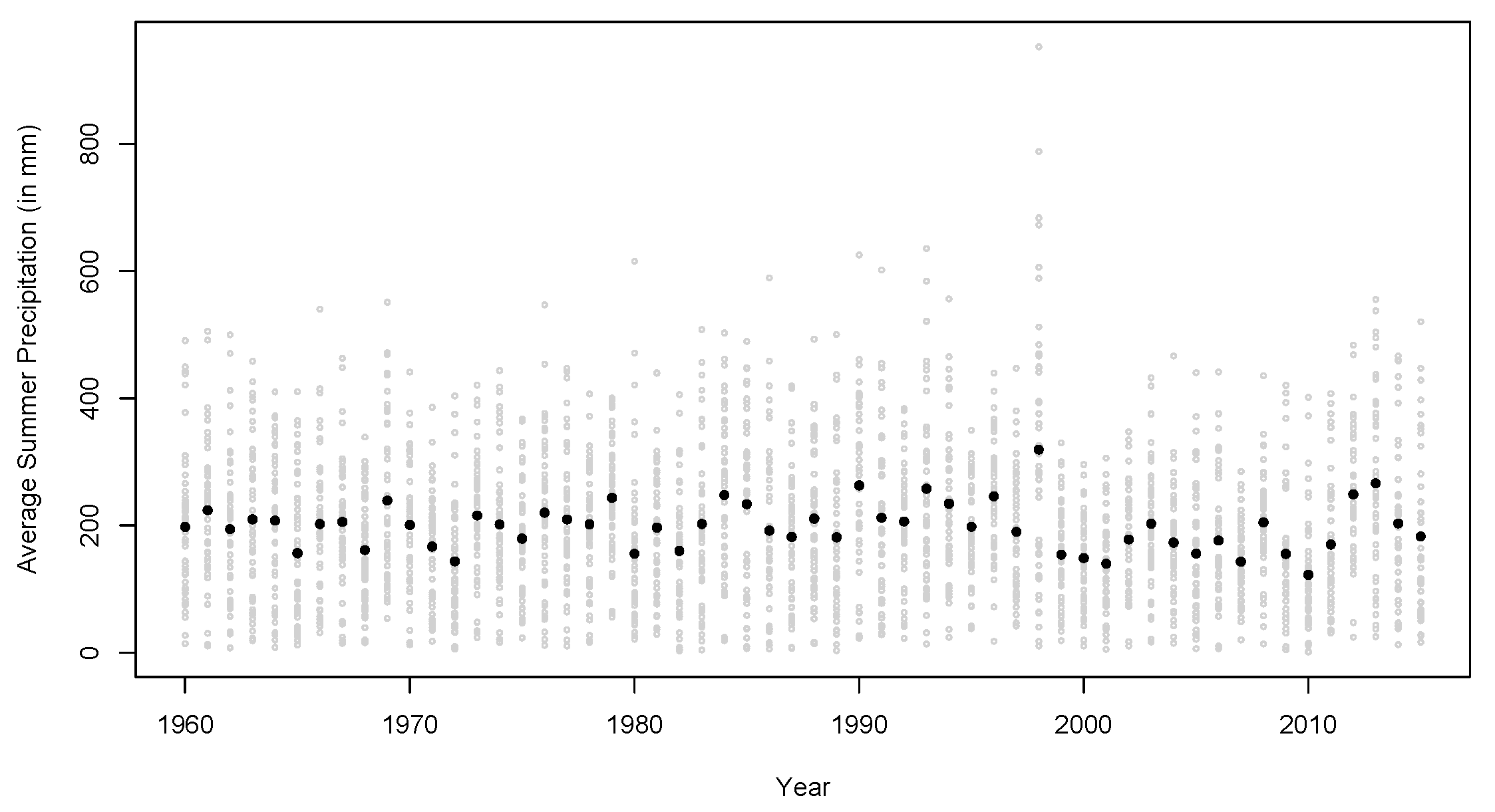
To understand ACDD and its relationship to other climate change indices, we use data from 50 stations in Neimenggu Province as an example. In Figure 2, we plot the total precipitation in the three summer months from 1960 to 2015 at each station, as well as the precipitation averaged over all stations in the province. It does not show any obvious trend or change over time.
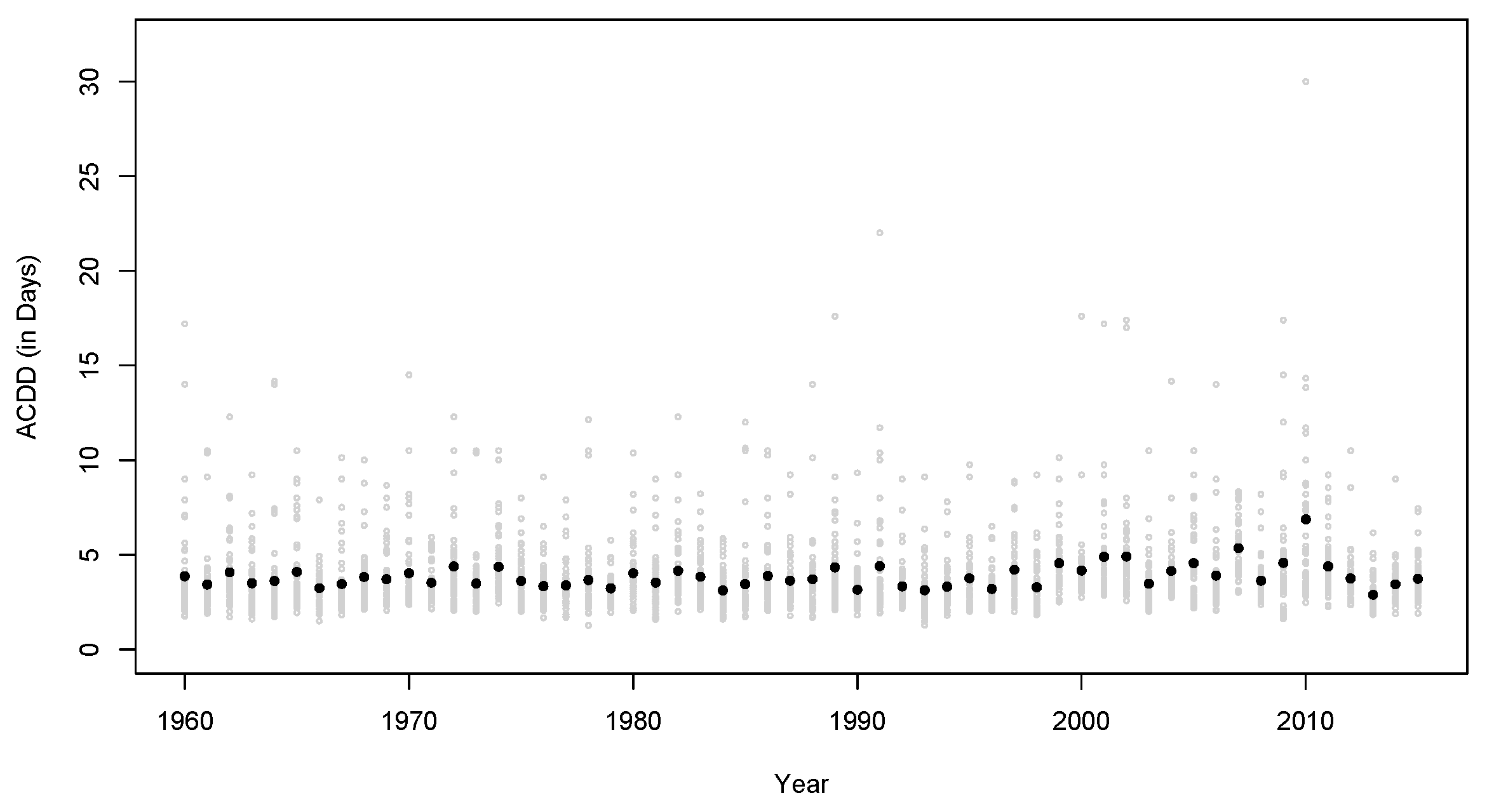
We plot the ACDD at each station and their average over all the stations in Figure 3. Here we see some increasing trends, particularly since 1990. We also see that 2010 was an extreme case when the ACDD exceeded 30 at some stations. These changes in precipitation were not clearly seen in the daily precipitations. In the next section, we will provide more analysis on the ACDD and the summer precipitations so that it becomes more evident that the ACDD can detect changes in precipitation patterns that the total precipitation does not.
2.3. Stochastic Ordering and Nonparametric Test
2.3.1. Stochastic Ordering of Random Variables
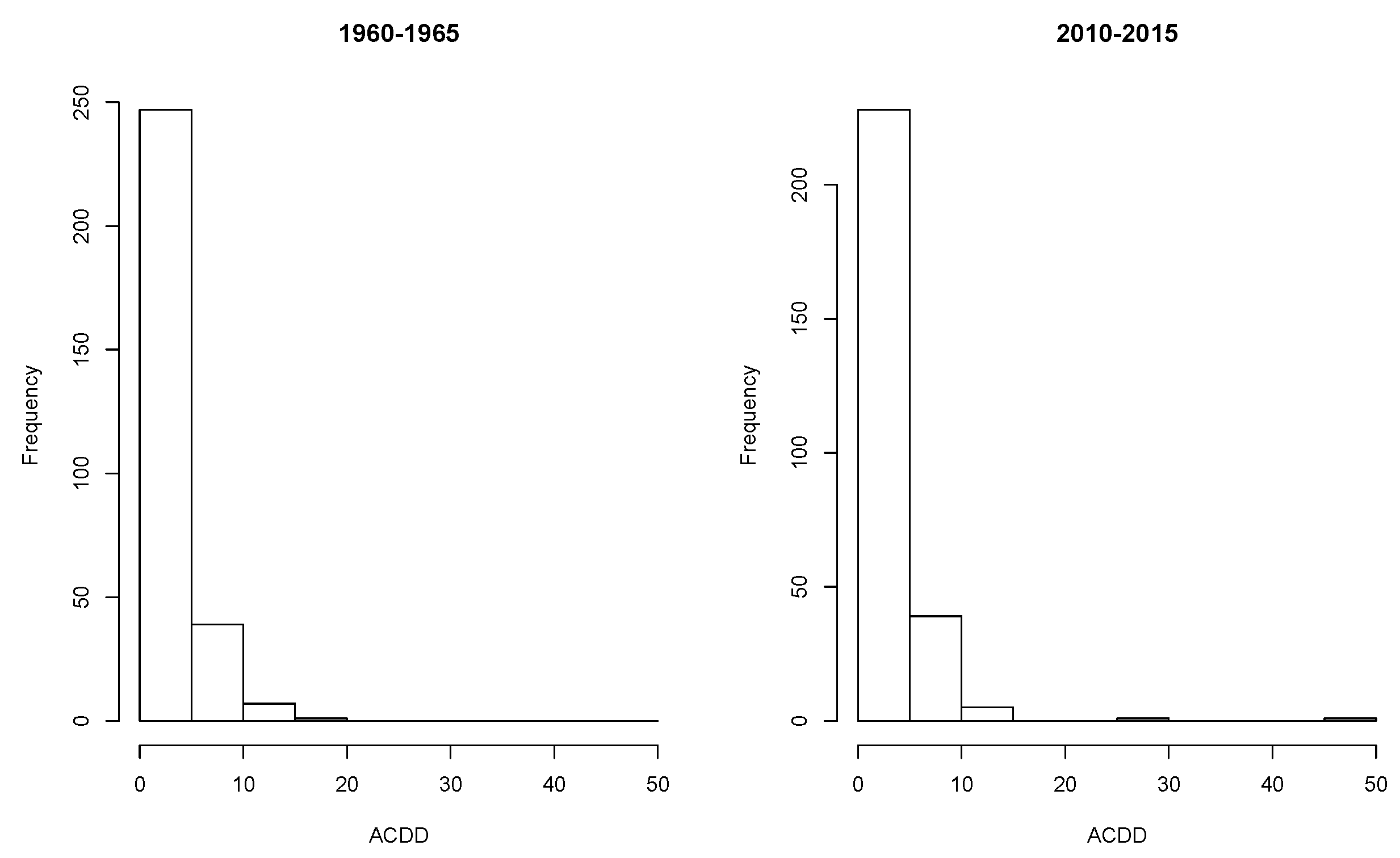
The change in ACDD over time can be translated into stochastic ordering, a probability concept to sort random variables in an increasing or decreasing order. To illustrate the concept, in Figure 4, we plot the histograms for ACDD at 50 stations in Neimenggu Province during the summer months in 1960–1965 and 2010–2015. The histograms seem to suggest that the ACDDs during 2010–2015 were “larger” than those during 1960–1965, and the ACDDs in both periods were skewed. This leads to the concept of stochastic ordering.
For two random variables and , is said to be stochastically larger than if for all , or equivalently, for all , where is the cumulative distribution function (cdf) of , . We denote the ordering by or . Hence, if , the cdf of is less than or equal to that of . For example, if has an exponential distribution with mean , then if . For our study, and may be the ACDD during the two periods of time, 2010–2015 and 1960–1965, respectively. Histograms in Figure 3 seem to suggest that was “larger” than . A formal statistical test would be needed to confirm that.
The cdfs are unknown in practice but can be estimated nonparametrically. Given a random sample from a probability distribution, the cdf can be estimated by the empirical cdf , which equals the number of ’s that are less than or equal to divided by .
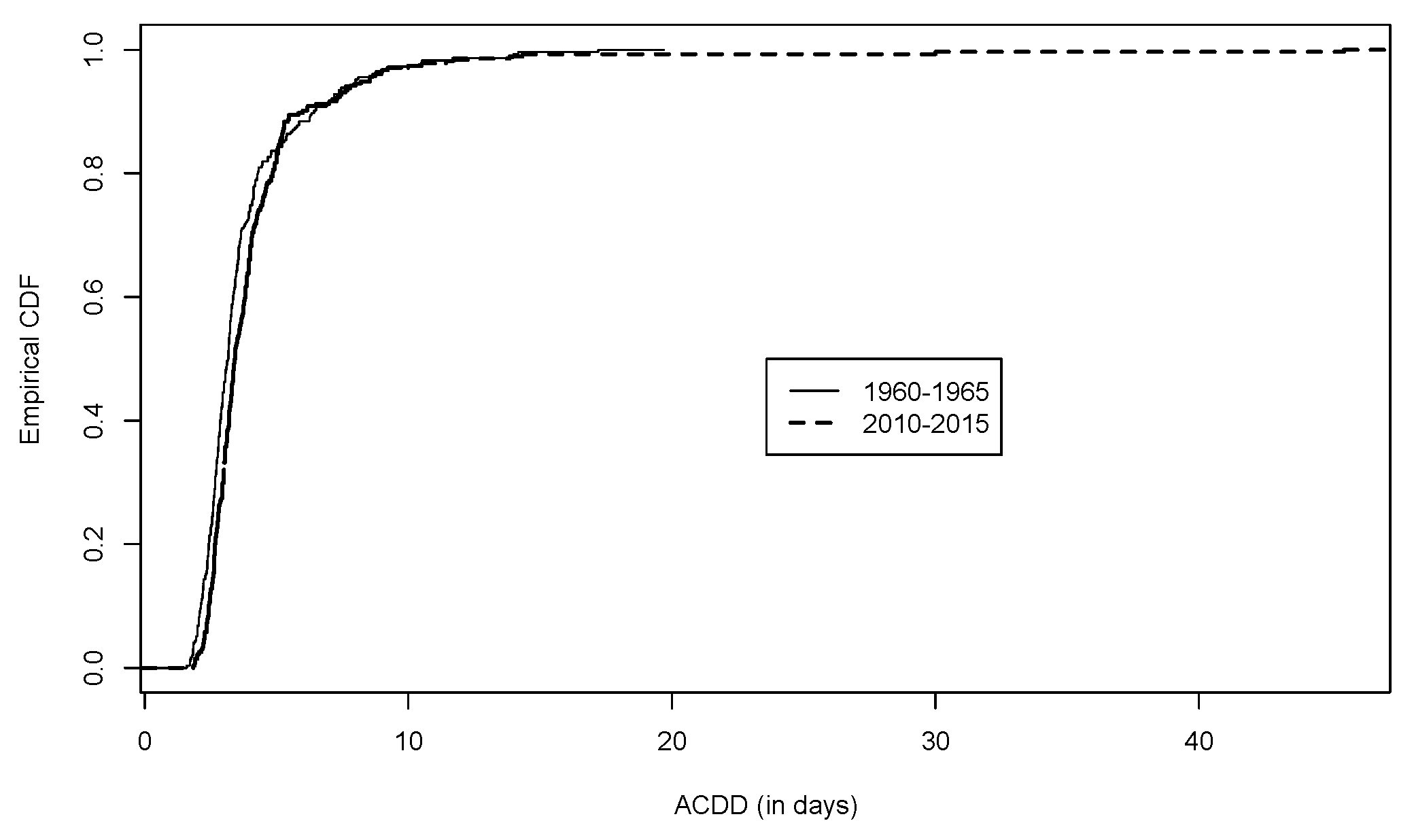
We plot the two empirical cdfs of the ACDD data in Figure 5, from which we see that the cdf for ACDD in 2010–2015 seemed to be lower than that in 1960–1965. However, this is an example where a formal statistical test is necessary to tell how significant the difference is. We will introduce such a formal statistical test for stochastic ordering in the next section.
2.3.2. Empirical Likelihood-Based Test for Stochastic Ordering
Given two random variables with cumulative, continuous distribution functions and , we would like to test the hypothesis
For example, is the cdf of ACDD in the summer months in 2010–2015 and is the cdf of ACDD in the summer months in 1960–1965.
A formal statistical test based on empirical likelihood was developed by EI Barmi and McKeague [44] and is shown to have more power than other test procedures. We employed this test to the above hypothesis. To introduce the test, it is necessary to introduce more notations. Suppose we are given a random sample of size from the cdf , and the two samples are independent. Let be the empirical cdf of the th sample. Let denote the cdf of the pooled sample, and be the weighted least squares projection of onto the set , with weights where [45]. Specifically, the projection minimizes
among all . If , the solution is . If , the weighted least squares is minimized by . Therefore, we have if , and if . Define
where any term raised to the zero power is set to 1. Then the test statistics is given by
Since is a step function, the above integral can be represented by a finite sum. Let , , be the unique values in the pooled sample and be the step jump at . More specifically,
Therefore, equals the number of sample data that equals devided by . Then the test statistics can be expressed as
where m denotes the total amount of unique values in the pooled sample.
Under the null hypothesis and assuming that the common distribution is continuous, EI Barmi and McKeague (2013) showed that has the limiting distribution (see Theorem 2 and Remark 2 in [44])
where is a standard Brownian bridge. They also provided critical values through simulations. For the significance level , the critical value was 1.821, and for , the critical value was . The null hypothesis is rejected if is greater than the critical value.
We note that this nonparametric test is particularly appropriate for skewed distributions because it does not make any assumptions on the shape of the distribution. When the data were skewed, as in Figure 3, it is generally inappropriate to apply a parametric test such as the Student’s t-test to compare the two means of ACDD because specific parametric assumptions about the probability distributions fail to hold. Some have attempted to use various parametric models to model the skewed distributions [46]. Nonparametric tests, such as the Mann-Kendall test, have been developed to test a monotone (increasing or decreasing) trend. However, our analyses indicate that the changes in ACDD over time may not follow a monotonic trend in some provinces. By comparing the ACDDs in different periods, it is possible to identify a non-monotonic trend.
2.3.3. Examples
As an example, we applied the test to the cdfs of ACDD shown in Figure 5. We will test the alternative hypothesis where and are the cdfs of ACDD in 2010–2015 and 1960–1965, respectively. was estimated by the empirical cdf that was obtained by the ACDD data during the summer months in 2010–2015 at the 50 stations and was estimated similarly. Since the pooled data from these stations were used, missing values at some stations are not a particular concern. The test statistics was 7.4181, which was greater than the critical value 3.185 at the significance level 0.01. There was significant evidence that the ACDD in 2010–2015 was stochastically larger than the ACDD in 1960–1965. This confirms what we observed in Figure 4 and Figure 5.
To see how this test compares with other statistical approaches, we applied the Mann–Kendall test to the time series of ACDD from 1960 to 2015. The test did not find any significant monotonic trend in ACDD. Therefore, in this case, the EI Barmi–McKeague test of stochastic ordering was able to reveal changes the Mann-–Kendall test does not.
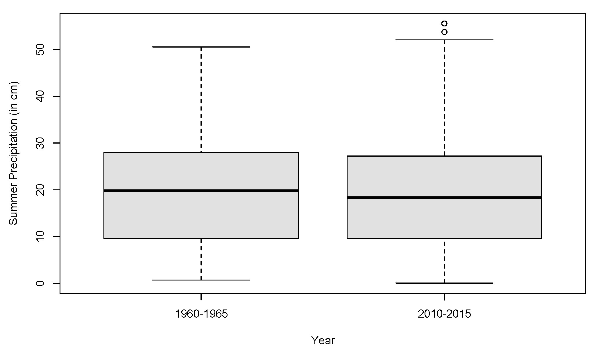
Next, we will see if there is any difference in the summer precipitations during the two periods of time in Neimenggu Province. We plot the precipitations in two box-plots in Figure 6, which shows the median, the 25th and 75th percentiles. There was no obvious difference in precipitations between the two periods of time, which was confirmed by a t-test (p-value = 0.995). The EI Barmi–McKeague test also showed no difference with a test statistic of 0.6191. These results suggest that ACDD, like CDD, is a useful measure for changes in precipitation that are otherwise not seen in the total precipitation.
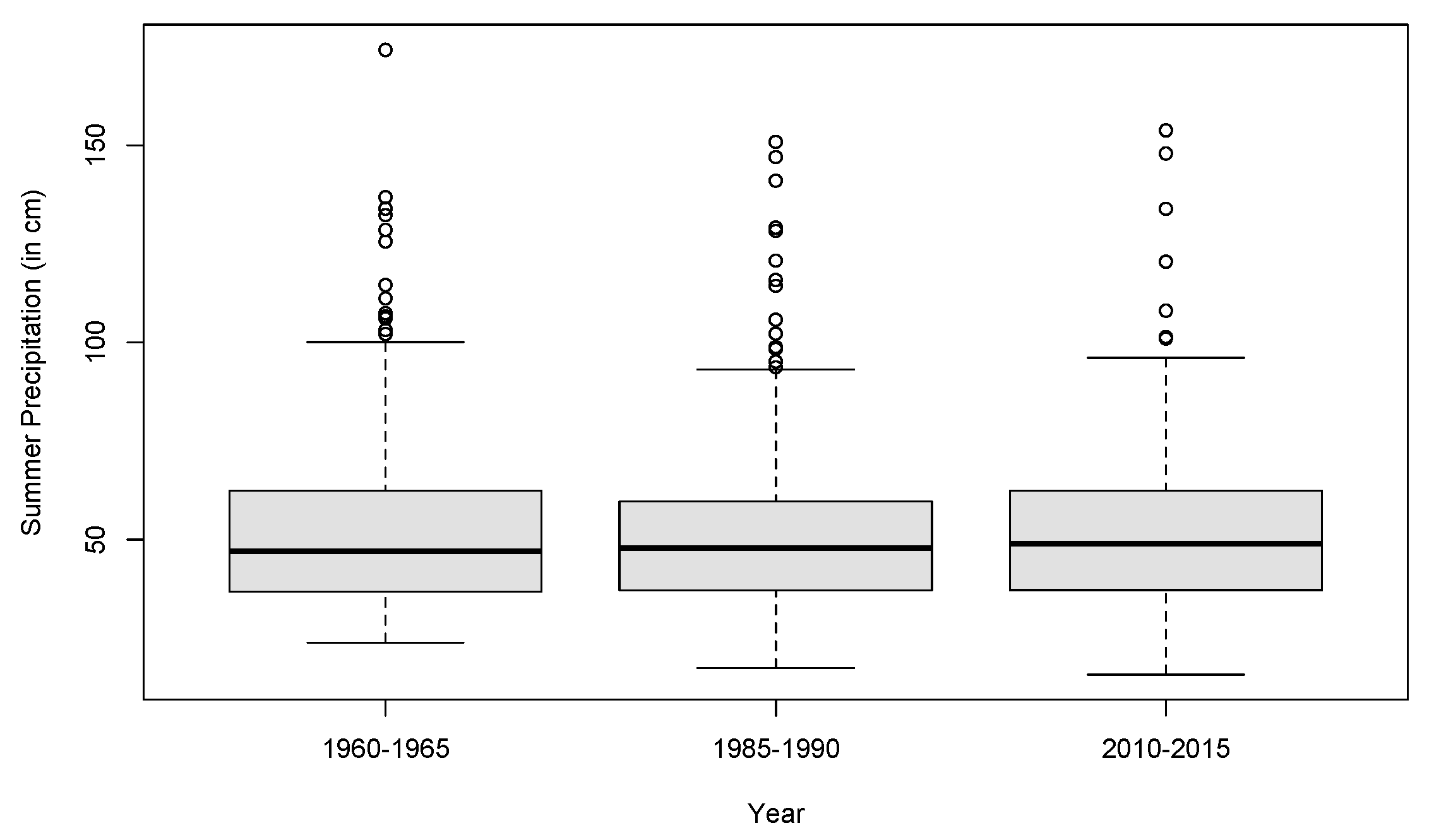
We now look at Sichuan Province in Southwestern China that has high precipitations in the summer months. The ACDD or CDD was not necessarily an index of drought for this province but provides a useful description of precipitation changes. In Figure 7, we plot the summer precipitations averaged over all stations for each of three periods of time 1960–1965, 1985–1990, and 2010–2015, which did not suggest any difference in the three periods. The ANOVA was performed, and the result reveals no significant difference. Since the data were right-skewed, we also applied the EI Barmi–McKeague test to compare summer precipitation for every pair of periods. Again, the tests suggest no significant difference in the summer precipitation.
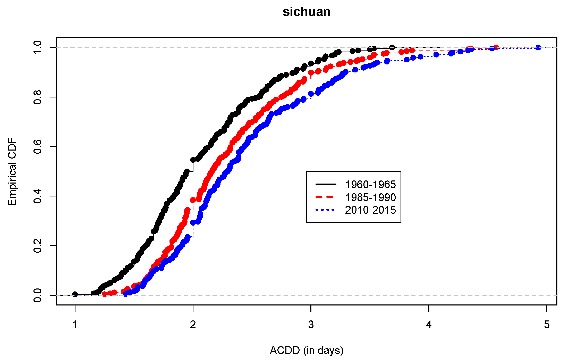
However, there was a clear difference among the ACDDs for the three periods, as seen in the empirical cdfs shown in Figure 8. The EI Barmi–McKeague test revealed a significantly increased order in ACDD from 1960–1965, to 1985–1990 and to 2010–2015. This example suggests that the ACDD and the test of stochastic ordering provide useful tools in detecting changes in precipitation.
3. Results
In this section, we applied the EI Barmi–McKeague test introduced in the previous section to compare the ACDDs during the summer months (June to August) in different periods for each province in China, similar to what we illustrated through Sichuan Province in the previous section. The data used in this work were the daily precipitation at 756 national key weather stations from 1960 to 2015, provided by the China Meteorological Administration. We choose three periods of time, 1960–1965, 1985–1990, and 2010–2015. The 20-year gap between the periods would render the ACDDs at two different periods independent, which is one assumption in the empirical likelihood-based test. The 6-year length of each period makes it a reasonable assumption that the CDDs within the period have an identical distribution. For each province, let , , and denote the cdf of the ACDD in the three periods. was continuous due to the definition of ACDD, and this continuity was a critical assumption for the asymptotic result to hold. This was the technical reason we employed the ACDD rather than other indices that take integer values. We tested three cases: , and .
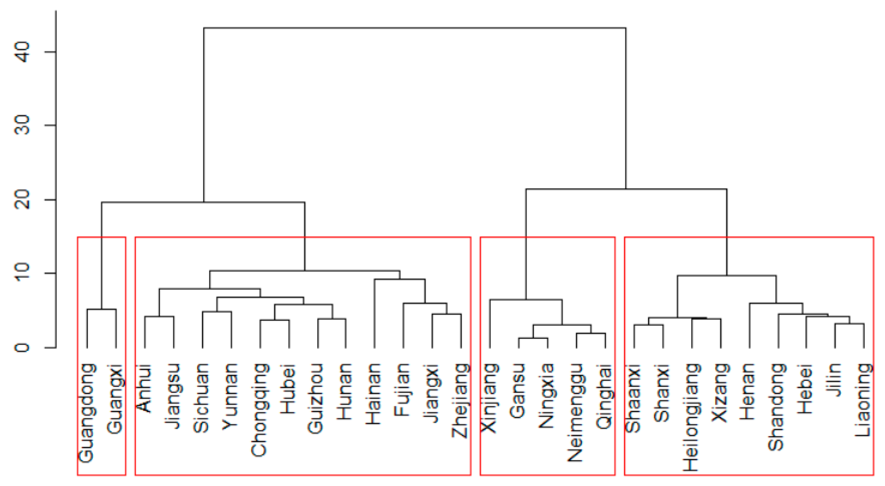
To help summarize the results for each province, we first clustered the provinces into different clusters where provinces in a cluster had similar daily precipitation. We employed hierarchical clustering [47] to divide the provinces into different clusters based on the summer precipitation. Hierarchical clustering is a method of cluster analysis that provides a hierarchy of clusters. We took the agglomerative or “bottom-up” approach, as implemented in the package hclust in R. Initially, each object was assigned to its own cluster, and then the algorithm proceeded iteratively so that at each stage, the two most similar clusters were merged. The algorithm continued until there was only one single cluster. The advantage of hierarchical clustering is that it allowed us to decide the level of hierarchy or the number of clustering that is most appropriate for application, and immediately obtain the clusters.
The data used in the hierarchical clustering were the average of summer precipitation per year over all stations in a province from 1960 to 2015. Ward’s minimum variance method was employed, and Euclidean distance was applied to measure the similarity. Here we chose the number of clusters in a way that the resulting clusters consist of contiguous provinces and were, hence, more interpretable. We then applied the tests to each province in the same way we demonstrated through Sichuan Province in the previous section. The resulting clusters are plotted in a dendogram in Figure 9, and the summary of clustering results is shown in Table 1.
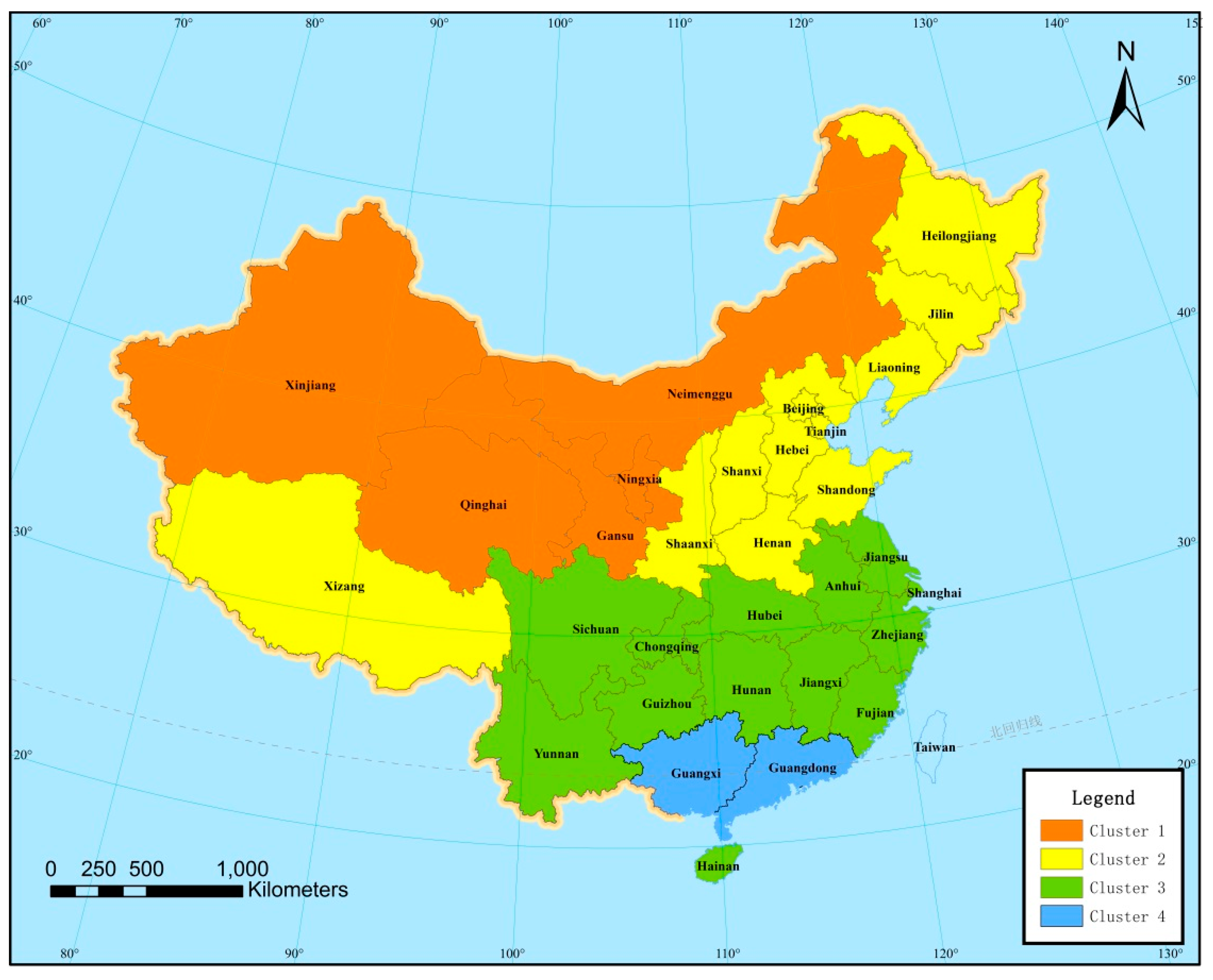
We plot spatial locations of these clusters in Figure 10. There are four clusters that contained five, nine, 12, and two provinces, respectively. Cluster 1 represents Northwest China, Cluster 2 consisted of provinces in north and northeast China, Cluster 3 consisted of provinces in Central, Southwest, and East China, and Cluster 4 contained Guangdong and Guangxi, which are located in South China. Precipitation increased from Cluster 1 to Cluster 4, and these clusters shift from north to south geographically. It agrees with the well-known fact that southern China receives more precipitation than the northern regions.
The test statistics for the EI Barmi–McKeague test are provided in Table 2, and those greater than the critical value at the 0.05 significance level are bold italic. We see that except three provinces (Xinjiang, Zhejiang, and Hunan), all provinces had ACDDs stochastically increasing from period 1 to either period 2 or period 3, or increasing from period 2 to period 3. More specifically, except five provinces (Gansu, Hubei, and the above three provinces), all other provinces experienced stochastically increased ACDD from period 1 to either period 2 or period 3. Fourteen provinces experienced stochastically increased ACDD from period 2 to period 3. Five provinces (Heilongjiang, Henan, Jilin, Sichuan, and Yunnan) had ACDD increasing from period 1 to period 2 and from period 2 to period 3. We think these results represent strong evidence that the precipitation patterns have changed over time. Namely, the average length of period between two adjacent precipitations tends to increase over time.
We also observed the spatial difference among the clusters. In Cluster 1, most provinces had stochastically larger ACDD in period 3 than that in period 2 or 1, but there was no significant difference between period 2 and 1, suggesting an increase in ACDD in more recent years. In Cluster 2, which consisted of nine provinces in northern and northeastern China, all provinces had stochastically larger ACDD in period 3 than that in period 1. ACDDs increased stochastically from period 1 to 2 in 6 of the nine provinces and also increased from period 2 to period 3 in six out of nine provinces. Three provinces had ACDDs strictly increasing from period 1 to period 2 and from period 2 to period 3. In Cluster 3, the ACDD increased stochastically from period 1 to period 2 or from period 1 to period 3 in nine out of 12 provinces and had no significant differences among the three periods in two provinces. In one province, the ACDD was stochastically larger in period 3 than in period 1, and there was no significant difference between period 1 and period 2. In Cluster 4, both provinces had ACDDs increasing stochastically from period 1 to period 2, and Guangdong also had a stochastically larger ACDD in period 3 than that in period 1. Cluster 4 had a similar change pattern of ACDD as that in Cluster 3.
4. Discussion
In this work, we introduced the stochastic ordering to the study of spatial and temporal changes in precipitation patterns and applied a formal statistical test for stochastic ordering. This test does not make any assumption on the shape of the probability distribution and is particularly appropriate for precipitation data which usually have skewed distributions. Therefore, it is a useful alternative approach to the current methods which often rely on some parametric assumptions.
The results of EI Barmi–McKeague test suggested that the average length between two adjacent precipitations in the summer months increased stochastically from 1960–1965 to either 1985–1990 or 2010–2015, or from 1985–1990 to 2010–2015 for all provinces in China except Xinjiang, Hunan, and Zhejiang. These results show a change in summer precipitation patterns in most regions. Specifically, the results imply that summer precipitation events tended to concentrate over time, prolonging the duration of dry spells between adjacent precipitations. The formal statistical test uncovered strong evidence of this change. This finding could possibly explain why China is experiencing an increasing frequency of extreme precipitation events. For example, 103 rainstorms occurred nationwide during the flood season from 2016 to 2018, according to the China Climate Bulletin, while many researchers have pointed out that average precipitation over China [48] and in many specific regions, such as Gansu Province [49], West China [50], Huashan Area [51], Hengduan Mountains region [52], had no obvious temporal trend. Overall, our study provides another point of view for looking into the change in precipitation patterns and can serve as a reference for water source management. The prolonged duration of a dry spell and the increased frequency of heavy precipitation open up interesting research problems in water runoff control and water preservation.
Our study can be generalized in a couple of ways. First, stochastic ordering combined with the EI Barmi–McKeague test can be applied to many other extreme climate indices (e.g., FD, R99p, SU, TXx, etc.) proposed by the World Meteorological Organization (WMO). Furthermore, the test can be used to compare climate indices in different spatial regions as well. It is implemented in R [53] and is available upon request. Second, the EI Barmi–McKeague test can be applied to test the ordering of multiple variables, for example, for any number of . The critical values of the test statistic are provided in [44] for up to 5. It, therefore, offers a way of comparing climate change indices in multiple time periods.
Finally, we note some limitations to our study. First, our results depend on the selections of the months and the particular time periods. We chose the summer months (June, July, and August) because the majority of provinces in China have the largest amount of precipitation during this season, and changes in precipitation patterns in this season have more significant consequences. The selection of different months or periods may result in different results. Hence, more comprehensive studies could be conducted. Second, the stochastic ordering only applies to a set of explicit time periods and does not apply to a temporal trend on a continuous time scale. On the other hand, this also provides some flexibility if the trend is non-monotonic or more complex to model.
Author Contributions
The two authors both contributed substantially to the manuscript. H.Z. proposed the methodology and is primarily responsible for writing the manuscript. N.N. performed all the statistical analysis and contributed to writing some parts of this manuscript. All authors have read and agreed to the published version of the manuscript.
Funding
This research received no external funding.
Conflicts of Interest
The authors declare no conflict of interest.
References
- Feng, P.; Wang, B.; Liu, D.L.; Xing, H.; Ji, F.; Macadam, I.; Ruan, H.; Yu, Q. Impacts of rainfall extremes on wheat yield in semi-arid cropping systems in eastern Australia. Clim. Chang. 2018, 147, 555–569. [Google Scholar] [CrossRef]
- Wang, P.; Deng, X.; Zhou, H.; Qi, W. Responses of urban ecosystem health to precipitation extreme: A case study in Beijing and Tianjin. J. Clean. Prod. 2018, 177, 124–133. [Google Scholar] [CrossRef]
- Scoccimarro, E.; Gualdi, S.; Bellucci, A.; Zampieri, M.; Navarra, A. Heavy Precipitation Events in a Warmer Climate: Results from CMIP5 Models. J. Clim. 2013, 26, 7902–7911. [Google Scholar] [CrossRef]
- Shalizi, Z. Water and urbanization. In Yusuf, S; The World Bank: Washington, DC, USA, 2008; pp. 159–184. [Google Scholar]
- Cao, L.; Pan, S.; Wang, Q.; Wang, Y.; Xu, W. Changes in extreme wet events in Southwestern China in 1960–2011. Quat. Int. 2014, 321, 116–124. [Google Scholar] [CrossRef] [Green Version]
- Wang, H.; Chen, Y.; Xun, S.; Lai, D.; Fan, Y.; Li, Z. Changes in daily climate extremes in the arid area of northwestern China. Theor. Appl. Climatol. 2013, 112, 15–28. [Google Scholar] [CrossRef]
- Wang, Y.; Xu, Y.; Lei, C.; Li, G.; Han, L.; Song, S.; Yang, L.; Deng, X. Spatio-temporal characteristics of precipitation and dryness/wetness in Yangtze River Delta, eastern China, during 1960–2012. Atmospheric Res. 2016, 172, 196–205. [Google Scholar] [CrossRef]
- Fischer, T.; Gemmer, M.; Lüliu, L.; Buda, S. Temperature and precipitation trends and dryness/wetness pattern in the Zhujiang River Basin, South China, 1961–2007. Quat. Int. 2011, 244, 138–148. [Google Scholar] [CrossRef]
- Jiang, F.; Hu, R.-J.; Wang, S.-P.; Zhang, Y.-W.; Tong, L. Trends of precipitation extremes during 1960–2008 in Xinjiang, the Northwest China. Theor. Appl. Climatol. 2013, 111, 133–148. [Google Scholar] [CrossRef]
- Li, Z.; Zheng, F.-L.; Liu, W.-Z.; Flanagan, D.C. Spatial distribution and temporal trends of extreme temperature and precipitation events on the Loess Plateau of China during 1961–2007. Quat. Int. 2010, 226, 92–100. [Google Scholar] [CrossRef]
- Qian, W.; Lin, X. Regional trends in recent precipitation indices in China. Theor. Appl. Clim. 2005, 90, 193–207. [Google Scholar] [CrossRef]
- Sun, L.-D.; Zhang, C.-J.; Zhao, H.-Y.; Lin, J.-J.; Qu, W. Features of Climate Change in Northwest China during 1961-2010. Adv. Clim. Chang. Res. 2013, 4, 12–19. [Google Scholar] [CrossRef]
- Wang, B.; Zhang, M.; Wei, J.; Wang, S.; Li, S.; Ma, Q.; Li, X.; Pan, S. Changes in extreme events of temperature and precipitation over Xinjiang, northwest China, during 1960–2009. Quat. Int. 2013, 298, 141–151. [Google Scholar] [CrossRef]
- Li, W.; Duan, L.; Luo, Y.; Liu, T.; Scharaw, B. Spatiotemporal Characteristics of Extreme Precipitation Regimes in the Eastern Inland River Basin of Inner Mongolian Plateau, China. Water 2018, 10, 35. [Google Scholar] [CrossRef] [Green Version]
- Liang, K. Spatio-Temporal Variations in Precipitation Extremes in the Endorheic Hongjian Lake Basin in the Ordos Plateau, China. Water 2019, 11, 1981. [Google Scholar] [CrossRef] [Green Version]
- Xiong, J.; Yong, Z.; Wang, Z.; Cheng, W.; Li, Y.; Zhang, H.; Ye, C.; Yang, Y. Spatial and temporal patterns of the extreme precipitation across the Tibetan Plateau (1986–2015). Water 2019, 11, 1453. [Google Scholar] [CrossRef] [Green Version]
- Trenberth, K.E.; Jones, P.D.; Ambenje, P.; Bojariu, R.; Easterling, D.; Klein Tank, A.; Parker, D.; Rahimzadeh, F.; Renwick, J.A.; Rusticucci, M.; et al. Observations. Surface and Atmospheric Climate Change; Chapter 3; Cambridge University Press: Cambridge, UK; New York, NY, USA, 2007. [Google Scholar]
- Alexander, L.V.; Zhang, X.; Peterson, T.C.; Caesar, J.; Gleason, B.; Tank, A.M.G.K.; Haylock, M.; Collins, D.; Trewin, B.; Rahimzadeh, F.; et al. Global observed changes in daily climate extremes of temperature and precipitation. J. Geophys. Res. Space Phys. 2006, 111, 111. [Google Scholar] [CrossRef] [Green Version]
- Peterson, T.C. Climate Change Indices. WMO Bull. 2005, 54, 83–86. [Google Scholar]
- Tao, Y.; Wang, W.; Song, S.; Ma, J. Spatial and Temporal Variations of Precipitation Extremes and Seasonality over China from 1961~2013. Water 2018, 10, 719. [Google Scholar] [CrossRef] [Green Version]
- Ávila, Á.; Guerrero, F.C.; Escobar, Y.C.; Justino, F. Recent Precipitation Trends and Floods in the Colombian Andes. Water 2019, 11, 379. [Google Scholar] [CrossRef] [Green Version]
- Lee, J. The consecutive dry days to trigger rainfall over West Africa. J. Hydrol. 2018, 556, 934–943. [Google Scholar] [CrossRef]
- Nastos, P.; Zerefos, C. Spatial and temporal variability of consecutive dry and wet days in Greece. Atmospheric Res. 2009, 94, 616–628. [Google Scholar] [CrossRef]
- Beniston, M.; Stephenson, D.B. Extreme climatic events and their evolution under changing climatic conditions. Glob. Planet. Chang. 2004, 44, 1–9. [Google Scholar] [CrossRef] [Green Version]
- Schmidli, J.; Frei, C. Trends of heavy precipitation and wet and dry spells in Switzerland during the 20th century. Int. J. Clim. 2005, 25, 753–771. [Google Scholar] [CrossRef]
- Zhou, B.; Liang, C.; Zhao, P.; Dai, Q. Analysis of Precipitation Extremes in the Source Region of the Yangtze River during 1960–2016. Water 2018, 10, 1691. [Google Scholar] [CrossRef] [Green Version]
- Heng, C.; Yoon, S.-K.; Kim, J.-S.; Xiong, L. Inter-Seasonal Precipitation Variability over Southern China Associated with Commingling Effect of Indian Ocean Dipole and El Niño. Water 2019, 11, 2023. [Google Scholar] [CrossRef] [Green Version]
- Suppiah, R.; Hennessy, K.J. Trends in total rainfall, heavy rain events and number of dry days in Australia, 1910–1990. Int. J. Clim. 1998, 18, 1141–1164. [Google Scholar] [CrossRef]
- Zhang, Y.; Jiang, F.; Wei, W.; Liu, M.; Wang, W.; Bai, L.; Li, X.; Wang, S. Changes in annual maximum number of consecutive dry and wet days during 1961–2008 in Xinjiang, China. Nat. Hazards Earth Syst. Sci. 2012, 12, 1353–1365. [Google Scholar] [CrossRef]
- Frich, P.; Alexander, L.; Della-Marta, P.; Gleason, B.; Haylock, M.; Tank, A.K.; Peterson, T. Observed coherent changes in climatic extremes during the second half of the twentieth century. Clim. Res. 2002, 19, 193–212. [Google Scholar] [CrossRef] [Green Version]
- Duan, Y.; Ma, Z.; Yang, Q. Characteristics of consecutive dry days variations in China. Theor. Appl. Climatol. 2017, 130, 701–709. [Google Scholar] [CrossRef] [Green Version]
- Zhang, J.; Chen, H.; Zhang, Q. Extreme drought in the recent two decades in northern China resulting from Eurasian warming. Clim. Dyn. 2019, 52, 2885–2902. [Google Scholar] [CrossRef] [Green Version]
- Shi, J.; Cui, L.; Wen, K.; Tian, Z.; Wei, P.; Zhang, B. Trends in the consecutive days of temperature and precipitation extremes in China during 1961–2015. Environ. Res. 2018, 161, 381–391. [Google Scholar] [CrossRef] [PubMed]
- Li, Y.-G.; He, D.; Hu, J.-M.; Cao, J. Variability of extreme precipitation over Yunnan Province, China 1960–2012. Int. J. Climatol. 2015, 35, 245–258. [Google Scholar] [CrossRef]
- Zhang, M.; Chen, Y.; Shen, Y.; Li, Y. Changes of precipitation extremes in arid Central Asia. Quat. Int. 2017, 436, 16–27. [Google Scholar] [CrossRef]
- Zhang, J.; Shen, X.; Wang, B. Changes in precipitation extremes in Southeastern Tibet, China. Quat. Int. 2015, 49–59. [Google Scholar] [CrossRef]
- Wang, B.; Zhang, M.; Wei, J.; Wang, S.; Li, X.; Li, S.; Zhao, A.; Li, X.; Fan, J. Changes in extreme precipitation over Northeast China, 1960–2011. Quat. Int. 2013, 298, 177–186. [Google Scholar] [CrossRef]
- Cheng, A.; Feng, Q.; Fu, G.; Zhang, J.; Li, Z.; Hu, M.; Wang, G. Recent changes in precipitation extremes in the Heihe River basin, Northwest China. Adv. Atmospheric Sci. 2015, 32, 1391–1406. [Google Scholar] [CrossRef]
- Zhang, K.; Pan, S.; Cao, L.; Wang, Y.; Zhao, Y.; Zhang, W. Spatial distribution and temporal trends in precipitation extremes over the Hengduan Mountains region, China, from 1961 to 2012. Quat. Int. 2014, 349, 346–356. [Google Scholar] [CrossRef]
- Shaked, M.; Shanthikumar, J.G. Stochastic Orders and their Applications; Associated Press: New York, NY, USA, 1994. [Google Scholar]
- Gupta, R.C.; Kirmani, S. Stochastic comparisons in frailty models. J. Stat. Plan. Inference 2006, 136, 3647–3658. [Google Scholar] [CrossRef]
- Di Crescenzo, A.; Pellerey, F. Stochastic comparisons of series and parallel systems with randomized independent components. Oper. Res. Lett. 2011, 39, 380–384. [Google Scholar] [CrossRef] [Green Version]
- Gong, D.-Y.; Shi, P.-J.; Wang, J.-A. Daily precipitation changes in the semi-arid region over northern China. J. Arid. Environ. 2004, 59, 771–784. [Google Scholar] [CrossRef]
- El Barmi, H.; McKeague, I.W. Empirical likelihood-based tests for stochastic ordering. Bernoulli 2013, 19, 295–307. [Google Scholar] [CrossRef] [PubMed] [Green Version]
- Robertson, T.; Wright, F.T.; Dykstra, R. Order Restricted Statistical Inference. In Probability and Statistics Series; Wiley: Chichester, UK, 1988; ISBN 978-0-471-91787-8. [Google Scholar]
- Li, L.; Yao, N.; Liu, D.L.; Song, S.; Lin, H.; Chen, X.; Li, Y. Historical and future projected frequency of extreme precipitation indicators using the optimized cumulative distribution functions in China. J. Hydrol. 2019, 579, 124170. [Google Scholar] [CrossRef]
- Strauss, D.J.; Hartigan, J.A. Clustering Algorithms. Biom. 1975, 31, 793. [Google Scholar] [CrossRef]
- Zuo, H.; Lyu, S.; Hu, Y. Variations trend of yearly mean air temperature and precipitation in China in the last 50 years. Plateau Meteorol. 2004, 23, 238–244. [Google Scholar]
- Wen, X.; Wu, X.; Gao, M. Spatiotemporal variability of temperature and precipitation in Gansu Province (Northwest China) during 1951–2015. Atmospheric Res. 2017, 197, 132–149. [Google Scholar] [CrossRef]
- Ye, J.-S. Trend and variability of China’s summer precipitation during 1955–2008. Int. J. Climatol. 2014, 34, 559–566. [Google Scholar] [CrossRef]
- Kai, H. Analysis of Precipitation Variation and Trend Forecast in Huashan Area of China. Sci. Discov. 2016, 4, 183. [Google Scholar] [CrossRef] [Green Version]
- Yu, H.; Wang, L.; Yang, R.; Yang, M.; Gao, R. Temporal and spatial variation of precipitation in the Hengduan Mountains region in China and its relationship with elevation and latitude. Atmospheric Res. 2018, 213, 1–16. [Google Scholar] [CrossRef]
- R Core Team. R: A Language and Environment for Statistical Computing; R Foundation for Statistical Computing: Vienna, Austria, 2018. [Google Scholar]
Figure 1.
Study area and locations of stations.

Figure 2.
Time series of the summer precipitation (in millimeters) at each station (gray circle) and their average over all stations (solid black) in Neimenggu Province from 1960 to 2015.
Figure 2.
Time series of the summer precipitation (in millimeters) at each station (gray circle) and their average over all stations (solid black) in Neimenggu Province from 1960 to 2015.

Figure 3.
The average number of consecutive dry days (ACDD) at each station (gray circle) and their average over all stations (solid black) in Neimenggu Province from 1960 to 2015.
Figure 3.
The average number of consecutive dry days (ACDD) at each station (gray circle) and their average over all stations (solid black) in Neimenggu Province from 1960 to 2015.

Figure 4.
Histograms for ACDD of summer months in 1960–1965 (left) and 2010–2015 (right) in Neimenggu Province.
Figure 4.
Histograms for ACDD of summer months in 1960–1965 (left) and 2010–2015 (right) in Neimenggu Province.

Figure 5.
The empirical cdfs of ACDD in two time periods, 1960–1965 (solid and thinner line) and 2010–2015 (dashed and thicker line) in Neimenggu Province.
Figure 5.
The empirical cdfs of ACDD in two time periods, 1960–1965 (solid and thinner line) and 2010–2015 (dashed and thicker line) in Neimenggu Province.

Figure 6.
Box-plot of summer precipitation (in cm) in Neimenggu Province during the two periods of time.
Figure 6.
Box-plot of summer precipitation (in cm) in Neimenggu Province during the two periods of time.

Figure 7.
Box-plot of summer precipitation (in cm) in Sichuan Province during the three periods of time.
Figure 7.
Box-plot of summer precipitation (in cm) in Sichuan Province during the three periods of time.

Figure 8.
Empirical cdf of ACDD (in days) in Sichuan Province in three periods. A lower cdf corresponds to a stochastically larger ACDD.
Figure 8.
Empirical cdf of ACDD (in days) in Sichuan Province in three periods. A lower cdf corresponds to a stochastically larger ACDD.

Figure 9.
Dendogram of hierarchical clustering analysis of summer precipitation in China.

Figure 10.
Spatial locations of clusters.


Table 1.
Clustering of provinces based on total precipitations in the summer months.
| Cluster | Province | Summer Precipitation |
|---|---|---|
| Cluster 1 | Gansu, Neimenggu, Ningxia, Qinghai, Xinjiang | 50–250 mm |
| Cluster 2 | Hebei, Heilongjiang, Henan, Jilin, Liaoning, Shaanxi, Shandong, Shanxi, Xizang | 200–600 mm |
| Cluster 3 | Anhui, Chongqing, Fujian, Guizhou, Hainan, Hubei, Hunan, Jiangsu, Jiangxi, Sichuan, Yunnan, Zhejiang | 300–800 mm |
| Cluster 4 | Guangdong, Guangxi | 600–1200 mm |
Table 2.
Test statistics for the stochastic ordering of ACDD in each province. Bold italic values indicate values greater than the critical value at the 0.05 significance level.
Table 2.
Test statistics for the stochastic ordering of ACDD in each province. Bold italic values indicate values greater than the critical value at the 0.05 significance level.
| Clusters | Provinces | |||
|---|---|---|---|---|
| Cluster 1 | Gansu | 0.0019 | 1.4623 | 4.5646 |
| Neimenggu | 0.587 | 7.4181 | 5.5302 | |
| Ningxia | 0.1293 | 2.814 | 9.601 | |
| Qinghai | 1.7112 | 4.3411 | 2.3174 | |
| Xinjiang | 0.6815 | 0.138 | 0.0949 | |
| Cluster 2 | Hebei | 1.3281 | 18.7565 | 15.0084 |
| Heilongjiang | 18.8994 | 44.9659 | 8.1306 | |
| Henan | 6.0975 | 29.7018 | 8.74 | |
| Jilin | 8.2339 | 26.0869 | 4.9394 | |
| Liaoning | 25.1472 | 30.7548 | 0.9905 | |
| Shaanxi | 0.7442 | 25.105 | 19.2106 | |
| Shandong | 26.7417 | 27.2558 | 1.1298 | |
| Shanxi | 0.5309 | 10.0733 | 7.4018 | |
| Xizang | 8.3363 | 8.4392 | 0.0729 | |
| Cluster 3 | Anhui | 1.821 | 3.7178 | 0.6346 |
| Chongqing | 1.7987 | 3.9871 | 1.3051 | |
| Fujian | 10.4399 | 3.0874 | 0.0494 | |
| Guizhou | 14.3116 | 17.2958 | 1.6873 | |
| Hainan | 8.1903 | 3.3558 | 0.0269 | |
| Hubei | 0.0231 | 0.7882 | 3.3235 | |
| Hunan | 0.7307 | 0.7244 | 0.2226 | |
| Jiangsu | 2.6904 | 1.7971 | 3.3392 | |
| Jiangxi | 3.615 | 0.1039 | 0.0000 | |
| Sichuan | 12.8098 | 24.027 | 3.2118 | |
| Yunnan | 5.4371 | 17.2401 | 3.5341 | |
| Zhejiang | 0.6524 | 0.538 | 0.1643 | |
| Cluster 4 | Guangdong | 4.1135 | 7.0419 | 1.0664 |
| Guangxi | 3.5708 | 0.417 | 0.0237 |
© 2020 by the authors. Licensee MDPI, Basel, Switzerland. This article is an open access article distributed under the terms and conditions of the Creative Commons Attribution (CC BY) license (http://creativecommons.org/licenses/by/4.0/).
Share and Cite
MDPI and ACS Style
Ni, N.; Zhang, H. A Study of Precipitation Patterns through Stochastic Ordering. Water 2020, 12, 351. https://doi.org/10.3390/w12020351
AMA Style
Ni N, Zhang H. A Study of Precipitation Patterns through Stochastic Ordering. Water. 2020; 12(2):351. https://doi.org/10.3390/w12020351
Chicago/Turabian StyleNi, Nan, and Hao Zhang. 2020. "A Study of Precipitation Patterns through Stochastic Ordering" Water 12, no. 2: 351. https://doi.org/10.3390/w12020351
Note that from the first issue of 2016, this journal uses article numbers instead of page numbers. See further details here.