Groundwater-Surface Water Interactions in “La Charca de Suárez” Wetlands, Spain
by
 , , ,
, , ,
Angela M. Blanco-Coronas
1,* ,
,
Manuel López-Chicano
1,
Maria L. Calvache
1,
José Benavente
1 and
Carlos Duque
2 1
Departamento de Geodinámica, Universidad de Granada, Avenida Fuente Nueva s/n., 18071 Granada, Spain
2
WATEC, Department of Geoscience, Aarhus University, Høegh-Guldbergs Gade 2, 8000 Aarhus C, Denmark
*
Author to whom correspondence should be addressed.
Water 2020, 12(2), 344; https://doi.org/10.3390/w12020344
Submission received: 6 December 2019
/
Revised: 17 January 2020
/
Accepted: 22 January 2020
/
Published: 25 January 2020
(This article belongs to the Special Issue Groundwater Resilience to Climate Change and High Pressure)
Abstract
:La Charca de Suárez (LCS) is a Protected Nature Reserve encompassing 4 lagoons located 300 m from the Mediterranean coast in southern Spain. LCS is a highly anthropized area, and its conservation is closely linked to the human use of water resources in its surroundings and within the reserve. Different methodologies were applied to determine the hydrodynamics of the lagoons and their connection to the Motril-Salobreña aquifer. Fieldwork was carried out to estimate the water balance of the lagoon complex, the groundwater flow directions, the lagoons-aquifer exchange flow and the hydrochemical characteristics of the water. The study focussed on the changes that take place during dry-wet periods that were detected in a 7-month period when measurements were collected. The lagoons were connected to the aquifer with a flow-through functioning under normal conditions. However, the predominant inlet to the system was the anthropic supply of surface water which fed one of the lagoons and produced changes in its flow pattern. Sea wave storms also altered the hydrodynamic of the lagoon complex and manifested a future threat to the conservation status of the wetland according to predicted climate change scenarios. This research presents the first study on this wetland and reveals the complex hydrological functioning of the system with high spatially and temporally variability controlled by climate conditions and human activity, setting a corner stone for future studies.
1. Introduction
Wetlands are considered some of the most productive and beneficial ecosystems in the world because of their high biological diversity [1] and the regulation of surface runoff, decreasing the risk of flooding and purifying inflowing waters [2,3]. However, many wetlands in Europe were considered low-production and unhealthy areas for humans for centuries and thus were drained [4,5]. Currently, wetlands are threatened, primarily due to the increase in economic activities and urban development.
Wetlands are particularly sensitive to changes affecting surface water (SW) or groundwater (GW) in their vicinity [6,7]. Knowledge of SW-GW interactions is essential for understanding their hydrodynamics [8,9,10] and to improve the management and protection. GW-SW fluxes have been traditionally quantified using field measurements or estimating each component of the water budget [11,12,13,14]. The connexion between a wetland system and an aquifer can change over the short term, controlled by the relative SW and GW heads [15,16]. Important variations can be produced by factors such as climate change [17] and to modifications on the water management due to regulation, channelization, upstream water abstractions [18,19]. Aquifer heterogeneities often generate irregular flow patterns, hindering the identification of groundwater inputs to wetlands (e.g., [20,21]). Additionally, groundwater exchange impacts on the water quality of wetlands [22].
La Charca de Suárez (LCS) is one of the few wetlands of south-east Spain [23] and the only coastal wetland in the region. LCS is a prime habitat for the wintering, nesting and migration of water birds that cross the Strait of Gibraltar, as well as for amphibian reproduction. In addition, LCS supports a number of endangered species in Spain, such as Fulica cristata [24]. It was classified as a Protected Nature Reserve by the regional government of Andalusia in 2009 owing to its high ecological value.
The LCS extension, like in other wetlands from Spain and Europe, has been considerably reduced since its appearance in the 14th–15th century [25]. The wetland was drained to increase the area of arable land and to eradicate diseases such as malaria. Also, from 1918 to 1985, the “Cambó” law was active in Spain, which granted the piece of land occupied by the wetland to anyone who drains it causing a loss of 60% of the wetlands in Spain since the 70s [26]. For these reasons, LCS wetland was decreased from more than 1000 ha registered in the XVIII century to 14 ha at the present. From 1980 to 2000, LCS was almost entirely disappeared due to urban development for tourism and the lack of water inlets due to infrastructure construction such as dams and irrigation channels. In 2000, a plan to recover the wetland was implemented and in 2009 it was recognized as Protected Nature Reserve [27].
One of the main characteristics of LCS is that it requires human intervention to maintain the sheet of water for the sustainability of the ecological system. The system receives inputs from surface water from irrigation channels generating highly variable conditions that can change regardless the weather conditions. Also, the management of the protected area requires a deep understanding of the water budget. So far, there is no information about the groundwater-surface water interaction of LCS or its water budget, and this is the first time that a study has focused on this area from a hydrological perspective. Because this system is affected by human management, during dry periods, the use of water is optimized to supply irrigation water reducing the inputs to the lagoons. The reaction of the system to these changes from and hydrological or chemical perspective can be considered as test anticipating predicted climate change scenarios in the long run [28].
The objective of this study is to determine the hydrological functioning of the LCS wetland and its interaction with Motril-Salobreña aquifer. As short-term changes can play an important role in the system, dry and wet periods will be analyzed and the methods for the local evaluation of the fluxes and water budget will be examined for a 7- and 5-month period of data collected, respectively.
2. Materials and Methods
2.1. Hydrological Settings
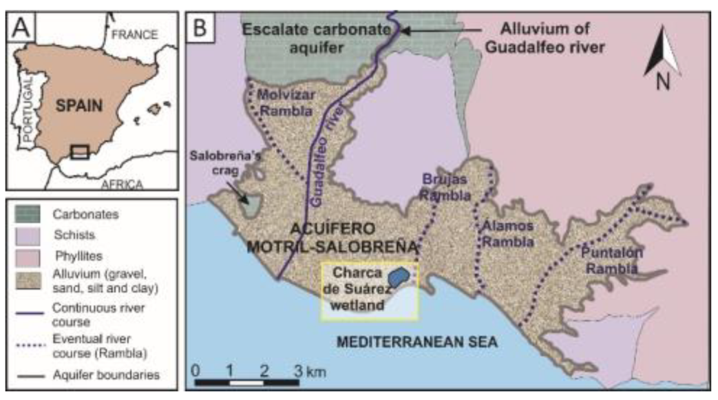
The Motril-Salobreña aquifer is located on the Mediterranean coast of south-east Spain in the province of Granada (Figure 1A). It is a detrital coastal aquifer with an extension of 42 km2 and means annual resources of 35 Mm3 [29]. It consists of poorly consolidated Quaternary detrital sediments discordantly overlying metamorphic rocks [30].
The aquifer is hydrogeologically bounded to the north by the alluvium of the Guadalfeo River and the Escalate carbonate aquifer and to the south by the Mediterranean Sea. Its lateral boundaries and the basement are composed of schists and phyllites of very low permeability (Figure 1B) [31]. The aquifer thickness ranges from 30 to 50 m in the northern sector (alluvial sedimentary environment) to more than 250 m in areas near the coastline (deltaic sedimentary environment) [31]. The lithology of the aquifer is characterized by alternating clays, silts, sand and gravel. In addition, the proportion of materials with higher hydraulic conductivity decrease north to south and east to west [32]. The direction of groundwater flow is north-south with a hydraulic gradient estimated between 1.6 × 10⁻³ and 5 × 10⁻³ [33]. The main natural recharge of the aquifer is produced by infiltration from Guadalfeo River [29,34] and by irrigation return flows [29,34], estimated at 11 Mm3/year and 16 Mm3/year, respectively. Other minor contributions are produced by lateral inlets from the Escalate aquifer (4 Mm3/year) and rainfall recharge (3–6 Mm3/year) [29] and by the alluvium from the river (1 Mm3/year) [35].
The main outlet is groundwater discharge from the aquifer to the sea, which is estimated to range from 17 to 26 Mm3/year [29,36,37,38]. Pumped outflows and, to a lesser extent, occasional river gains, in its final stretch, are also important.
The Guadalfeo River, with a drainage basin of 1290 km2, is the main watercourse that runs through the aquifer, with a mixed pluvio-nival regime. It collects a large part of the waters that drain the southern slope of the Sierra Nevada mountain massif (3482 m a.s.l. of maximum altitude). The Guadalfeo River Plain is an area with intense agricultural activity. A complex network of irrigation channels covers the entire surface of the Motril-Salobreña aquifer and transports the waters previously derived from the Guadalfeo River. In this region, the flood irrigation method is commonly applied, which uses more water than that required by plants [33]. Part of the excess water infiltrates and becomes part of irrigation return flows, and the other part flows as surface runoff and is recovered again by the irrigation channels that ultimately discharge it into the sea.
The climatic characteristics of the basin are highly variable over time and space. Its climate ranges from subtropical Mediterranean in the coast to high-mountain Mediterranean in high-altitude areas. The average precipitation is 400 mm/year in the coast and 1000 mm/year in the high-altitude areas of Sierra Nevada, primarily as snow. The wet seasons occur during the autumn and winter months, whereas summer months are extremely dry.
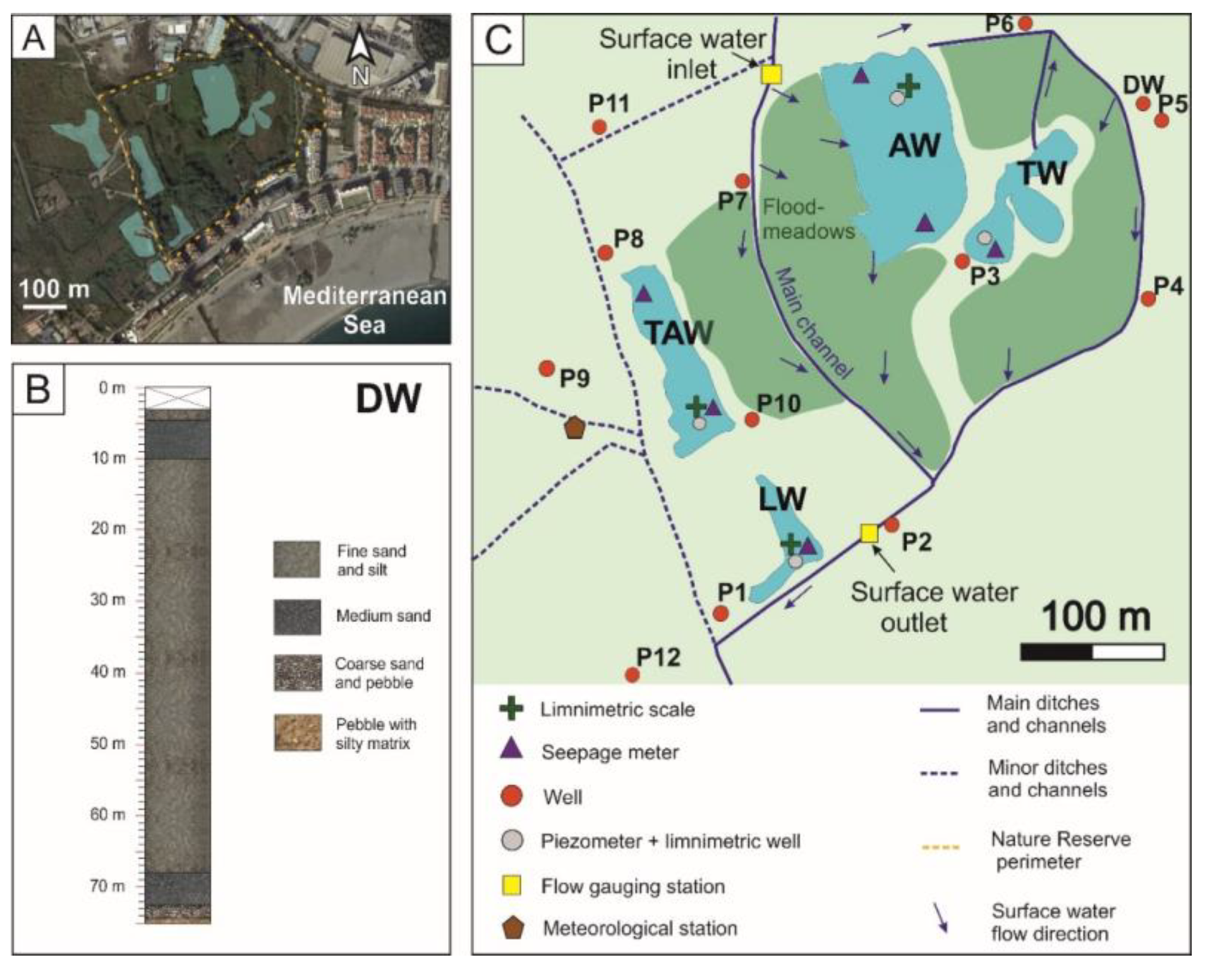
The LCS wetland is located in the southern border of the Motril-Salobreña aquifer, in its discharge zone to the sea. This specific area of the aquifer belongs to the former Guadalfeo river mouth. The local lithology of the first 75 meters of the aquifer is known based on a 75 m deep well (Well DW) (Figure 2B). It consists of alluvial sediments (fine sands and some pebbles) and prodeltaic silty sediments. Although the sediments are the same for all the study area, the proportion and spatial distribution can vary widely as it is normal in these sedimentary environments. The lagoon complex encompasses several waterbodies, but this study focuses on those within the perimeter of the protected area (Figure 2A), namely, Aneas (AW), Lirio (LW), Taraje (TAW) and Trébol (TW). The lagoons have various sizes ranging from 11,400 m2 to 1800 m2 and maximum depths ranging from 3.5 m to 1.2 m. These lagoons are surrounded by topographically low areas that sporadically flood during wet periods and that can even connect the lagoons.
Surface water inlets occur north of the reserve due to the main channel that collects surplus irrigation water from the Guadalfeo River Plain and surface runoff from the drainage basin. This channel crosses the protected area from north to south and feeds vegetation-covered areas naturally prone to flooding known as flood meadows. The water moves by surface runoff until reaching some of the lagoons, depending on the degree of flooding of the flood meadows. The main channel and others collect the water surplus of the lagoons, merging south of the reserve and flowing directly to the sea (Figure 2C). These channels are directly excavated without any impermeabilization and can contribute to the interaction with the groundwater. The channels are 0.7 m deep and they would require very high water table conditions, close to the groundwater flooding of the area to participate in this interaction. In this study, they have not been studied as it has been not observed a major impact over the system functioning but they remain as a research question to explore in the future.
2.2. Monitoring Network
A set of measuring stations was established to monitor changes in surface water, groundwater and weather conditions. This was the first time that the water inputs to LCS were quantified and required of several additional measuring points after the initial monitoring net design. One of the challenges working in protected areas with endangered species is the restriction for fieldwork activities and the limitation in the time periods that access to the lagoons is granted. This affected directly to the research activities in the lagoons to reduce the ecological disturbance (i.e., nesting periods).
Hydrometeorological data: These data were collected from a Davis Vantage Pro2 Plus wireless weather station. Precipitation, atmospheric pressure, temperature, wind speed and direction and solar radiation measurements were taken every 30 min (Figure 2C) with a resolution and accuracy of each parameter represented in Table 1.
Discharge data: Two gauging stations were built to measure the inflow and outflow discharge of the reserve. They consisted of a V-shaped weir and of a limnimetric scale. In addition, a pressure sensor was installed to measure the water surface height every hour. These data were transformed into discharge using rating curves constructed with measurements taken manually at each station. The correlation coefficients (R2) of the rating curves are 0.78 for inflow and 0.92 for outflow.
Groundwater level data: A total of 10 wells, 7 with depths of 3 m, 1 with a depth of 7 m and 2 with depths of 20 m, all 11 cm in diameter, were drilled using the rotary core drilling technique specifically for this project. In addition, 4 piezometers 11 cm in diameter were also installed at the bottom of each lagoon by nailing them to the bed at a depth of 0.5 m to estimate vertical hydraulic gradients. The wells are screened in their entire length and the lagoon piezometers have a 30 cm screen. Due to the lack of stability of the sediments, it was assumed that the screens were sealed immediately by to the collapsing during the drilling. In spite of the proximity to the groundwater discharge zone to the sea it was not observed vertical flow, likely because of the shallow depth reached in most of the wells. In wells P1, P2, P3, P4, P5, P6, P7 and P8 (Figure 2C), pressure sensors were installed to measure the groundwater level hourly. Monthly measurements were taken in P9, P10, P11 and P12 and in the lagoon piezometers.
Limnimetric data: Water level variations in each lagoon were assessed using sensors installed in limnimetric tubes slotted throughout their length. Hourly readings were taken and verified using measurements taken from the monthly limnimetric scales.
Water level data from gauging stations, lagoons, wells and piezometers were recorded by Seametrics LevelSCOUT smart pressure sensors (Resolution: 0.34 mm; Accuracy: ±5 mm). These data loggers were complemented with a BaroSCOUT barometric pressure sensor (Resolution: 0.34 mm; Accuracy: ±5 mm) and were calibrated with manual level measurements taken with an OTT HydroMet KL010 contact gauge. All measurements were referenced to the absolute zero of the mean sea level with a GPS Leica System 1200+ (Vertical resolution: 6mm; Accuracy: ±0.55–2 cm).
Direct measurements of exchange flow: 6 Lee-type seepage meters [39] were installed inside the lagoons, 4–15 m distance from the shoreline. Due to the verticality of the lagoon margins, seepage meters were 0.7–1 m below the water surface. A 3 m long tube separated each seepage meter from the collection bag to avoid footsteps near the measurement of the affection to vertical hydraulic conductivity [40]. Each bag was half-filled with tap water prior to the installation and a valve remained it closed during removal and while unattached. The weight variation was measured at the same 6 sites once per month, recording gains or losses as a function of the predominant relationships between the surface and groundwater. In each field campaign, measurements were repeated at approximately the same time of the day. In this work, the flow was considered positive or negative from the point of view of the lagoons. Positive if there was water inflow from the aquifer to the lagoons and negative if there was water outflow from the lagoons to the aquifer.
Water sampling for hydrochemical analysis: Water samples were collected at 5 points (in surface and groundwater inlets and outlets and in lagoons AW and TW), and in situ measurements of physicochemical water parameters (electrical conductivity, EC, temperature, T, pH, Eh, O2) were performed. Chemical analysis of major and some minor components was performed at the Centre of Hydrogeology of the University of Málaga using a Compact IC Pro 881 ion chromatograph and a Shimadzu TOC-VCSN + TNM − 1 carbon analyzer.
Seawaves height information: The hourly data of sea-waves height were obtained from State Harbours (Spanish Ministry of Development) from the SIMAR point close to the study area. The data was obtained from a high-resolution numerical modelling which integrates the basic transport equation: WAN wave generation model [41].
2.3. Evaporation Calculation
Penman equation (Equation (1)) [42], which estimates evaporation from free water surfaces by combining the energy balance with the mass transfer method, has been applied to accurately estimate evaporation from shallow wetlands [43]:
Where is the daily evaporation, is the slope of the daily mean saturated vapour pressure, is the daily net radiation on the evaporation surface, is the psychrometric constant, is the latent heat of vaporisation, and is the correction factor of wind action. The parameters were calculated using the climatic variables collected from the weather station. Both evaporation and precipitation were applied to the extension of the wetlands, but also to the flood meadows. The main channel feeds them in the north and collects water in the south; Therefore, gains by precipitation and losses by evaporation over the flood meadows must be considered in the calculation of the water balance.
2.4. Water Balance of the Lagoons
The water balance of the lagoons was calculated from January 2019 to May 2019, considering the principle of mass conservation:
where Qin and Qout are the surface water inflow and outflow to the lagoon complex, P is precipitation, is evaporation, ΔS is the variation in water storage in the lagoons, and GWFin and GWFout are groundwater flow into and out of the lagoons, respectively. ΔS is positive when water storage increases in the lagoons and negative when water is lost. Given that:
where GWF is the net exchange flow between the lagoons and the aquifer. GWF is positive when most groundwater flow was produced from the aquifer to the lagoons (GWFin > GWFout) and negative when most groundwater flow was produced from the lagoons to the aquifer (GWFout > GWFin). Substitution into (2) results in the following equation:
All variables of the equation were measured, except for GWF, which is commonly estimated indirectly or by residual approximation [44]. In this study, the soil water storage variation was disregarded due to the permanent state of high moisture.
2.5. Groundwater Contour Maps
Groundwater level elevation data were used to draw detailed groundwater contour maps by natural neighbour interpolation (ArcGIS 10.1). The maps were compared with specific measurements taken in the lagoons and with the estimated water balances as an additional tool to verify the results.
3. Results
3.1. Water Balance of the Lagoons
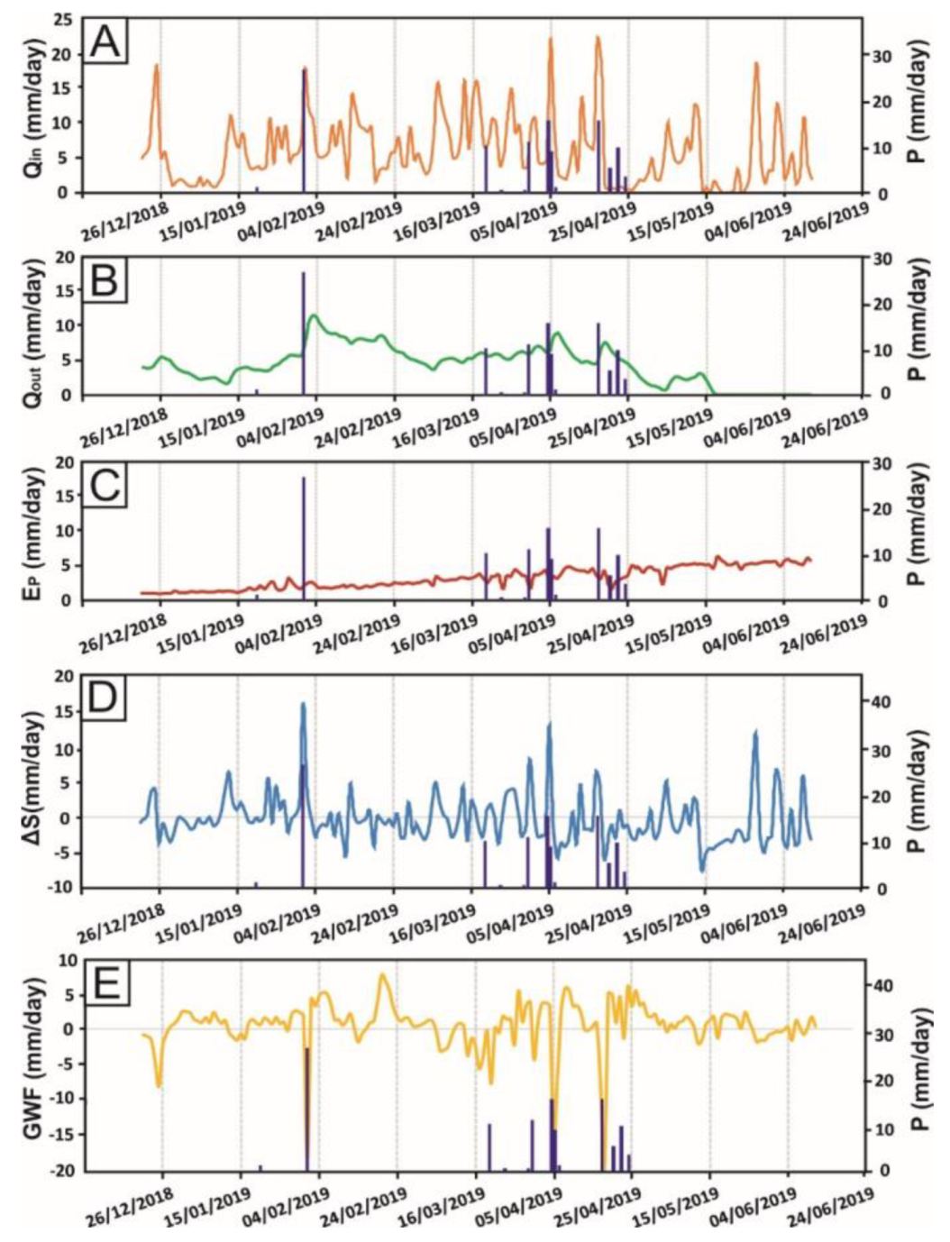
The water balance from January to May 2019 was calculated using average daily data (Figure 3). Surface water flow records (Figure 3A,B) showed differences in discharge between inlet and outlet stations. SW inflow (Qin) ranged from 0 to 50 l/s in short periods of time, and these variations were related to precipitation and to the irrigation management of the basin upstream of the reserve. SW outflow (Qout) did not experience the recorded short-term variations in Qin, and it ranged from 0 to 15 L/s. Only major and long-term increases in discharge were recorded, albeit less pronounced and with a few days lag because the wetlands temporarily retained surface water, which delayed the transfer of the water mass from the inlet to the outlet [45]. The calculated daily evaporation () (Figure 3C) ranged from 0.8 to 6.7 mm, reaching its highest values in May and the lowest values in January, marking an increasing trend. Daily data on storage variation (ΔS) (Figure 3D) were similar to those on Qin. The increase in inflow triggered a rapid response of the water level height in the lagoons and an increase in the amount of storage water. The daily findings of net exchange flow between surface water and groundwater (GWF) are mostly positive (Figure 3E); that is, the aquifer feeded the lagoons. In turn, sporadic negative peaks that coincided with periods of precipitation and/or sudden increases of Qin were recorded. These peaks were inverse to those of Qin and ΔS. When there were precipitation and a great contribution of surface water, the groundwater level was overcome by the limnimetric level and the net exchange flow was from the wetland to the aquifer.
The total monthly values of the variables of the water balance equation (Equation (4)) in the 5 study months show that Qin was the main water inlet to the system (Table 2). P accounted for 9% of the total inflow during the 5 months. April was the rainiest month, and P reached 57% of the total inflow. Except in March, the total monthly values of GWF were always positive because GWFin exceeded GWFout most days of the month. This results from the fact that GWF was only negative for short periods of time and it did not modify the sign of the monthly value of GWF. In March, the combined value of Qin and P increased, and GWF was negative. Qout was the main outlet of the system until May, when flow ceased. , however, progressively increased to become the main outlet of the system (83%). ΔS was highly variable, with positive and negative oscillations throughout the study period.
Errors in measuring and estimating hydrologic components were analyzed in the estimation of water balance because the results could vary widely [46]. The mean absolute errors calculated were: 41 mm for Qin, 0.2 mm for P, 10 mm for Qout, 13 mm for and 2 mm for ΔS. The water balances calculated with extreme errors (minimum inputs and maximum outputs or maximum inputs and minimum outputs) differed from the results of the Table 2 and the range in the water-balance uncertainty is shown in the Table 3.
3.2. Characterisation of the Lagoon Functioning
3.2.1. Lagoon Levels
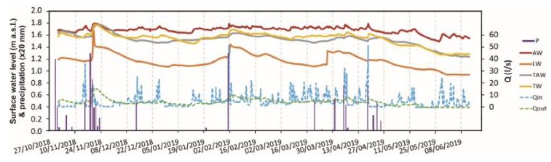
The records of limnimetric levels (Figure 4) showed that the absolute levels of the lagoons were not equal, decreasing from north to south. The lagoon with the highest level was AW, followed by TW and TAW, with LW having the lowest level. LW and TAW had very gentle curves, excluding the sporadic peaks of LW (see the explanation of Figure 5). The AW level was more varied, with sporadic peaks identified in Qin records. TW showed an intermediate behaviour between AW and TAW-LW.
Lagoon levels increased with the Qin, but the reaction rate was not the same in all lagoons. The AW level instantaneously increased on the same day when inflow peaks. TW reacted more slowly, and its level peaks approximately two days later than AW. Finally, the LW and TAW levels showed no response to the increase in Qin most times, and when it did, it took more days to react than the other lagoons.
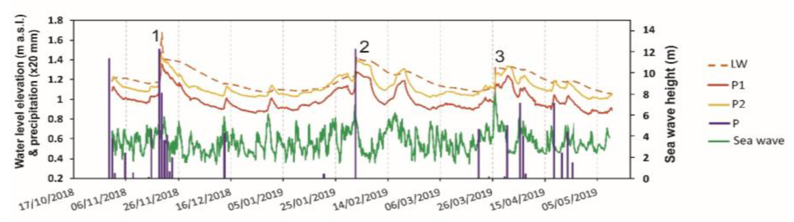
However, three instantaneous and sudden jumps in the water level were recorded in the LW lagoon (the lagoon located closest to the coastal edge), which were not recorded in the other lagoons. In addition, these jumps were even more clearly identified in wells P1 and P2 (Figure 5). Field observations showed increases in water levels on days when flooding occurred in the coastal strip. Coastal floods are usually related to precipitation and/or wind and wave storms [47,48,49]. Comparisons between limnimetric records in LW and water table records in P1 and P2, as well as precipitation and wave records in the sector (Figure 5), show that these sudden increases in the lagoon LW were clearly related to episodes of strong waves that cause floods near the coast and a local sea-level rise that was also transmitted to the water table, as recorded by wells located closer to the sea. Peaks 1 and 2 also coincided with intense rainfall; however, no precipitation was recorded in peak 3; therefore, the lagoon water level rise resulted exclusively from wave action. This action must have occurred locally because it was not recorded in other lagoons or wells.
3.2.2. Groundwater Levels
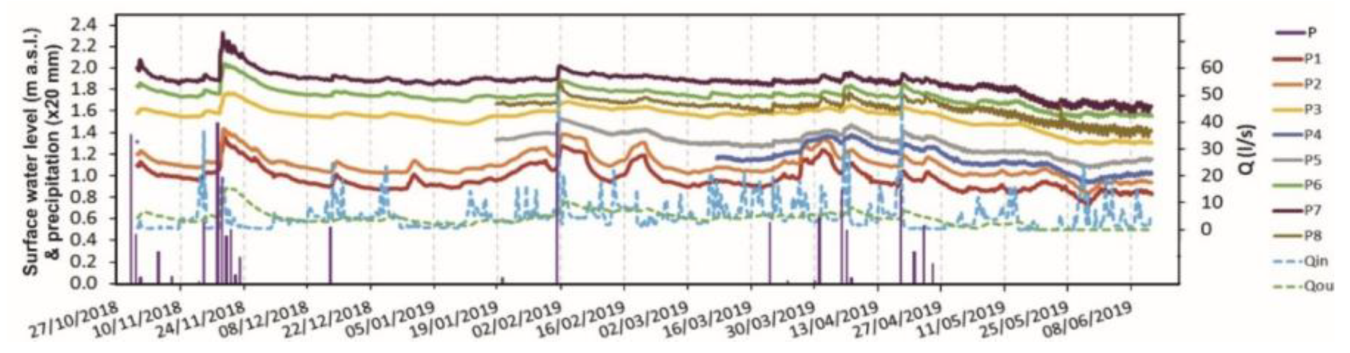
The water table elevation recorded in the wells (Figure 6) decreased from north to south, similarly to the limnimetric levels (Figure 4). In general, surface and groundwater levels varied similarly throughout the study period. They showed a constant trend until early May 2019, when they clearly began to decline.
Normally, short-term abrupt increases were preceded by an increase in Qin, which in turn depended on P and irrigation return flows. The response in the groundwater level was faster in northern wells than in southern wells. The groundwater level responded a few hours slower than the AW water level, albeit from 1 to 4 days faster than the other lagoons.
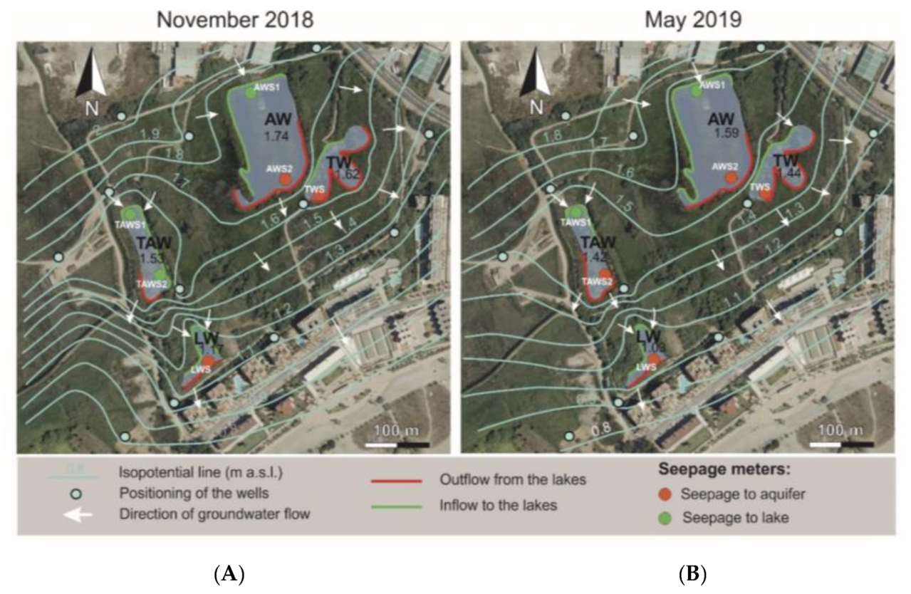
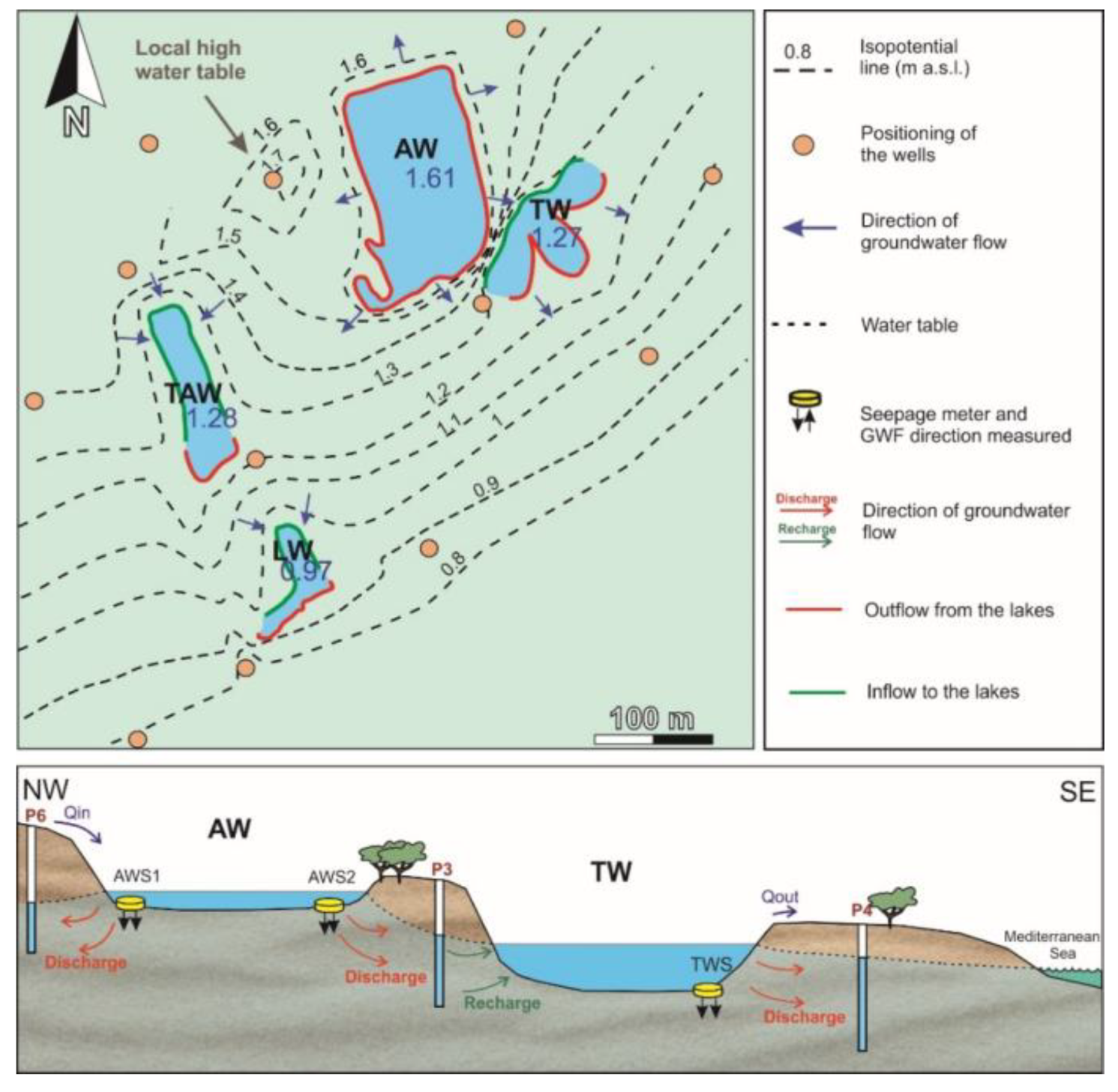
The groundwater contour map shows the flow when both surface and groundwater levels were high (November 2018) and low (May 2019) (Figure 7). The general flow patterns were similar in both cases. According to the maps, the lagoons were connected to the aquifer, despite spatial variations in the interaction between the two bodies of water. Discharge to the lakes occurred in the northern boundary of the lagoons and recharge to the aquifer in the southern boundary; therefore, they are flow-through lagoons. The differences between high and low water levels resulted from variations in the hydraulic gradient because the gradient was higher in November than in May.
3.2.3. Direct Measurements of Exchange Flow
The 6 seepage meters installed in the LCS wetland showed differences in GWF depending on their positioning (Figure 7). The AWS1 and TAWS1 seepage meters highlighted that the aquifer fed the lagoons in the northern section of the lagoons. Conversely, the AWS2, TWS and LWS seepage meters indicated negative flow; that is, recharge from the lagoons to the aquifer occurred in the southern section of the lagoons. In addition, temporal variations were observed, as shown in TAWS2, which measured a positive flow in November 2018 (inflow to the lakes) and a negative flow in May 2019 (outflow from the lakes). Therefore, the field data supported the groundwater contour maps and the groundwater flow patterns of the isopotential maps.
3.3. Hydrochemistry
The concentration of elements in water samples was similar in all sampling points (Figure 8), which indicated a close correlation between surface and groundwater throughout the aquifer. The salinity of lagoon AW was similar to that of surface water inlets (SW Inlet) and outlets (SW outlet), which confirms the fast connection between surface water and said lagoon that had already been revealed by the water level and Qin measurements. Groundwater (GW) had a lower concentration of elements than the other sampling points. Last, the TAW lagoon was the sampling point with the highest salinity. This may seem contradictory since their feeding depended exclusively on groundwater; therefore, they should have had more similar concentration values. The higher concentration of the lagoons fed by the aquifer may be due to the fact that they underwent less water renewal (longer residence time) and that evaporation produced an enrichment in salts in those lagoons (e.g., [50]). These variations in water composition indicated that in detail, there were notable differences in hydrological functioning between the different lagoons of the study area.
4. Discussion
The water balance of the wetland shows that surface water flow was the main inlet to the system, accounting for 82% of the total feeding of the lagoons during the five-month study period. Net groundwater exchange was calculated in every study month and accounted for 9% of the inlet to the lagoons. Precipitation accounted for 9% of the total inlet, although no precipitation occurred in some months. Evaporation and surface water outflow were the outlets of the system with similar total percentages of 60% and 40% respectively. Significant changes in the values of water balance components occurred in March that was especially wet during 2019. The main inlet to the system was Qin which increased up to 93%, and GWF became an outlet of the system (19%). Therefore, it could be deduced that recharge to the aquifer dominated in the especially wet months when surface-water levels were high, as it has been shown in other wetlands [51,52]. The results of the water balance are based on the mean values of each balance component. The analysis of the errors indicates a high degree of uncertainty under the most extreme consideration of error. Despite this, the best-estimated balance is near to the mean.
This water balance is only considering 5 months so it might not be totally representative of a full hydrological year. However, during the period studied, wet and dry short periods have been identified and the quantitative and qualitative differences between both indicate the need for longer-term studies in these areas due to the high climatic seasonality. This region is characterized by periods of several years with alternation of climatic conditions, for example droughts can be extended for several years while wet periods can exceed or be shorter than a hydrological year. This has been shown by calculating Standardized Precipitation Indexes (SPI) [38] or by the analysis of water table elevations trends [38] that usually do not return to the starting level after a hydrological year. Considering this, the time period presented here was sufficient to cover dry and wet short periods and represented a starting point for understanding seasonality over LCS. Longer-term studies are required to evaluate the effect of droughts and longer wet periods and to compare water budgets in LCS for different hydrological years.
Although flow patterns with vertical upward components have been studied in other parts of the Motril-Salobreña aquifer [33,53], but in this study we did not identify these patterns. The explanation could be due to the shallow depth of the wells and the lagoons and therefore, the regional discharge of the aquifer to the coast did not impact the water level measurements neither the groundwater-surface water interactions. The low-permeability sediments deposited on the lagoon-aquifer interface could have greatly influenced seepage rates [40], as well as the presence of organic sediments observed in other locations [54,55]. These could be the causes of the low percentage of the net groundwater exchange obtained in the water balance. The measurements of groundwater level and limnimetric levels (Figure 4 and Figure 6) reveal that the four lagoons were connected to the Motril-Salobreña aquifer, although they depended on groundwater differently. The LW, TAW and TW lagoons responded more strongly to changes in groundwater levels; therefore, it can be argued that their feeding mainly depended on groundwater. Lagoon AW, located in a more northern position and closer to the surface water inlet channel, must have had a considerable surface water feeding because variations in limnimetric levels were correlated with the inlet channel and with precipitation. Water from the channel flowed along the flood meadow as surface runoff and reaches AW. The small differences in the hydrochemical characteristics between TW lagoon and SW inlet also supported the existence of a fast connection between the AW lagoon and the surface water. However, the lagoons exclusively fed by groundwater, like TAW, were characterized by higher salinities, even higher than groundwater, showing the slow water renewal.
Daily data on water balance components of the lagoons (Figure 3) highlight that net groundwater flow to the wetland reacted inversely to SW inflow, precipitation and water storage. Precipitation and the surface discharge peaks produced limnimetric level increases in the AW lagoon. The net groundwater flow value calculated for the entire reserve, which was usually positive and low values (0–7 mm/d), decreased. Because AW is the largest lagoon in the reserve, in those cases when the water level at AW increased largely and the hydraulic gradient inverted sharply, the net groundwater flow drastically decreased and became negative (with values up to −20 mm/d). Discharge of great magnitude occurred from the lagoons complex to the aquifer for a few days. Inversions ended when the infiltration to the aquifer stabilized the groundwater and limnimetric levels at the same height. This was the reason why there was a sequence of rises in the limnimetric levels of the wetlands: the water level increased instantaneously in AW when the SW inflow increased, followed by the increased in the groundwater level due to the flow from AW to the aquifer and, ultimately, to the lagoons that depended on groundwater feeding (Figure 4 and Figure 6). The water level at TW increased faster than those at LW and TAW due to the proximity of TW to AW.
An anomalous phenomenon occurred on the coast and altered the hydrodynamic of the lagoon complex. The functioning of LW changed when there were flooding episodes in the coastal strip, caused by precipitation and/or sea wave storms. Sea level rises produced jumps in the water level that was also transmitted to the limnimetric level of the LW lagoon (Figure 5). However, this signal was barely recorded in the limnimetric level data of the remaining lagoons, probably because they are few more meters inland from the coast. On the other hand, all the lagoons may be affected in the near future according to the sea level rise forecasts due to climate change [28].
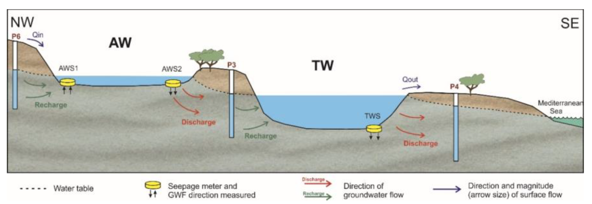
The groundwater contour maps and the seepage measurements (Figure 7) indicate that the lagoons received groundwater in the northern section of their basins and lost surface water to the aquifer in the southern section. Therefore, they were flow-through lagoons under normal conditions (Figure 9).
Starting at the end of April, the groundwater and limnimetric levels decreased continuously, reaching their minima since the beginning of the study period (Figure 4 and Figure 6). Under these conditions of very low water levels, the flow pattern in the AW lagoon changed from flow-through lagoon to influent lagoon. Similar changes in the interactions between wetlands and groundwater have been observed in other studies [56,57]. When Qin increased, surface water feeding of the AW lagoon increased, reflected in a sudden rise in water level, even exceeding the groundwater level in all sectors of the lagoon. The main channel behaved like an influent stream and produced a local high water table in the western sector of AW (Figure 10). Thereby inverting the hydraulic gradient in the northern sector of the lagoon, which became an aquifer feeding point. Drastic changes of groundwater flow direction were studied by other authors indicating temporal variations in the hydrodynamic functioning of lagoons [58].
Thus, the climate variability impacted on the interactions between GW-SW directly, mostly through changes in precipitation and evaporation. Indirectly, through changes in the inlets surface water. The SW availability was also strongly linked with the management of the basin water resources. Human activity controls the Guadalfeo river flow and the crop water, on which the two main recharge sources of the aquifer depends (infiltration from the river and the irrigation return flow). Successively, GW was an important inlet to the wetland, along with the surplus irrigation water. Then, LCS-Motril-Salobreña aquifer system is very sensitive to temporal variation caused by climate conditions and anthropic influence.
5. Conclusions
The groundwater-surface water interaction in LCS wetlands presented a variety in the distribution of both spatially and temporally. The LW, TAW and TW lagoons (groundwater-fed only) always showed a flow-through functioning with groundwater inflows in the northern section and the aquifer recharged in the southern section. The AW lagoon (mixed water inlets) showed different flow patterns depending on the hydrological conditions. Under normal conditions, it behaved as a flow-through lagoon; however, during wet periods, the rise in the limnimetric level changed AW to an influent lagoon.
During the study period, the net exchange flow, which is the total water that remains in the system, indicated that surface water was the predominant inlet to the system (82%) compared with the groundwater (9%). This proportion remained even during the driest periods. Nevertheless, the seepage meters and the hydrochemical analysis suggested that groundwater was dominant for most of the lagoons (LW, TAW and TW) while only AW lagoon had a mixed input of groundwater and surface water. This means that surface water inflow in AW lagoon played a highly relevant role in the water budget of the system. AW lagoon recharged the aquifer and might have even been partially the origin of the groundwater that later would recharge the other lagoons.
The anthropic water supply conducted through the main channel produced changes in the flow pattern of AW lagoon, which would have been flow-through type under natural conditions. The extra supply of water associated with human activity increased the water storage of the wetland, recharged the subjacent aquifer and prevented saltwater intrusion due to the proximity to the coastline.
LCS is an example of how the anthropic influence may affect a wetland in different manners. While human actions were responsible for almost the disappearance of the wetland by draining it and changing the land uses reducing its extension, the current management is maintaining the required hydrological conditions for sustaining the ecological equilibrium and also protects Motril-Salobreña aquifer from saltwater intrusion.
Author Contributions
Conceptualization: A.M.B.-C., M.L.C, M.L.-C. and C.D.; Methodology: A.M.B.-C., M.L.C., M.L.-C., J.B. and C.D.; Formal Analysis: A.M.B.-C., M.L.C., M.L.-C. and C.D.; Investigation: A.M.B.-C., M.L.C., M.L.-C., J.B. and C.D.; Resources: M.L.C., M.L.-C., J.B. and C.D.; Writing—original draft preparation: A.M.B.-C.; Writing—review and editing: A.M.B.-C., M.L.C., M.L.-C., J.B. and C.D.; Visualization: A.M.B.-C.; Supervision: M.L.C., M.L.-C. and C.D.; Project Administration: M.L.C. and M.L.-C.; Funding Acquisition: M.L.C. and M.L.-C. All authors have read and agreed to the published version of the manuscript.
Funding
This study was supported by grant CGL2016-77503-R from the Ministry of Economy and Competitiveness (MINECO), cofounded by the European Regional Development Fund (ERDF) of the European Union (EU), and the RNM-369 research group of the regional government of Andalusia.
Acknowledgments
The authors thank the staff of LCS, from the municipality of Motril, for their help in installing and surveilling the monitoring network and Ángel Perandrés, technician in the Department of Geodynamics of the University of Granada, for his availability when building seepage meters and installing weirs. The authors also thank the State Harbours (Ministry of Public Services, Government of Spain) for providing the sea wave height dataset.
Conflicts of Interest
The authors declare no conflict of interest.
References
- Misch, W.J.; Gosselink, J.G. Wetlands, 2nd ed.; Van Nostrand Reinhold: New York, NY, USA, 1993. [Google Scholar] [CrossRef]
- Richardson, C.J. Wetlands ecology. In Encyclopedia of Environmental Biology; Nierenberg, W.A., Ed.; Academic Press: New York, NY, USA, 1995; Volume 3, pp. 535–550. [Google Scholar]
- Misch, W.J.; Gosselink, J.G. Wetlands, 3rd ed.; John Wiley & Sons: Hoboken, NJ, USA, 2000. [Google Scholar] [CrossRef]
- Jones, T.A.; Hughes, J.M.R. Wetland inventories and wetland loss studies: A European perspective. In Waterfowl and Wetland Conservation in the 1990s; Moser, M., Prentice, R.C., van Vessem, J., Eds.; IWRB Special Publication No. 26; IWRB: Slimbridge, UK, 1993; pp. 164–170. [Google Scholar]
- McCovie, M.R.; Christopher, L.L. Drainage District Formation and the Loss of Midwestern Wetlands, 1850–1930. Agric. Hist. 1993, 67, 13–39. [Google Scholar]
- Suso, J.; Llamas, M.R. Influence of groundwater development on the Doñana National Park ecosystems. Hydrol. J. 1993, 141, 239–269. [Google Scholar] [CrossRef]
- Syphard, A.D.; Garcia, M.W. Human- and beaver- induced wetland changes in the Chickahominy River watershed from 1953 to 1993. Wetlands 2001, 21, 342–353. [Google Scholar] [CrossRef]
- Richter, B.D.; Baumgartner, J.V.; Powell, J.; Braun, D.P. A method for assessing hydrologic alteration within ecosystems. Conserv. Biol. 1996, 10, 1163–1174. [Google Scholar] [CrossRef] [Green Version]
- Shaffer, P.W.; Kentula, M.E.; Gwin, S.E. Characterization of wetland hydrology using hydrogeomorphic classification. Wetlands 1999, 19, 490–504. [Google Scholar] [CrossRef]
- Zedler, J.B. Progress in wetland restoration ecology. Trend Ecol. Evol. 2000, 15, 402–407. [Google Scholar] [CrossRef]
- Doss, P.K. The nature of a dynamic water table in a system of non-tidal, freshwater coastal wetlands. J. Hydrol. 1993, 141, 107–126. [Google Scholar] [CrossRef]
- Mills, J.G.; Zwarich, M.A. Transient groundwater flow surrounding a recharge slough in a till plain. Can. J. Soil Sci. 1986, 66, 121–134. [Google Scholar] [CrossRef] [Green Version]
- Ramberg, L.; Wolski, P.; Krah, M. Water balance and infiltration in seasonal floodplain in the Okavango delta, Bostwana. Wetlands 2006, 26, 677–690. [Google Scholar] [CrossRef]
- Mendoza-Sanchez, I.; Phanikumar, M.S.; Niu, J.; Masoner, J.R.; Cozzarelli, I.M.; McGuire, J.T. Quantifying wetland-aquifer interactions in a humid subtropical climate region: An integrated approach. J. Hydrol. 2013, 498, 237–253. [Google Scholar] [CrossRef]
- Rosenberry, D.O.; Winter, T.C. Dynamics of water-table fluctuation in an upland between two praire potholes wetlands in North Dakota. J. Hydrol. 1997, 191, 266–289. [Google Scholar] [CrossRef]
- Amoros, C.; Bornette, G. Connectivity and bioicomplexity in waterbodies of riverine floodplains. Freshw. Biol. 2002, 47, 761–776. [Google Scholar] [CrossRef]
- Wurster, F.C.; Cooper, D.J.; Sanford, W.E. Stream/aquifer interactions at Great Sand Dunes National Monument, Colorado: Influences on interdunal wetland disappearance. J. Hydrol. 2003, 271, 77–100. [Google Scholar] [CrossRef]
- Walker, K.F.; Thoms, M.C.; Sheldon, F. Effects of weirs on the littoral environment of the River Murray, South Australia. In River Conservation and Management; Boon, P.J., Calow, P., Petts, G.E., Eds.; John Wiley and Sons: New York, NY, USA, 1992; pp. 271–292. [Google Scholar]
- Jolly, I.D. The effect of river management on the hydrology and hydroecology of arid and semi-arid floodplains. In Floodplain Processes; Anderson, M.G., Walling, D.E., Bates, P.D., Eds.; John Wiley and Sons: New York, NY, USA, 1996; pp. 577–609. [Google Scholar]
- Freeze, R.A.; Witherspoon, P.A. Theoretical analysis of regional groundwater flow 3: Quantitative interpretations. Water Resour. Res. 1967, 4, 581–590. [Google Scholar] [CrossRef]
- Krabbenhoft, D.P.; Anderson, M.P. Use of a numerical ground-water flow model for hypothesis testing. Groundwater 1986, 24, 49–55. [Google Scholar] [CrossRef]
- Lewandowski, J.; Meinikmann, K.; Nützmann, G.; Rosenberry, D. Groundwater- the disregarded component in lake water and nutrient budgets. Part 2: Effects of groundwater on nutrients. Hydrol. Proc. 2015, 29, 2922–2955. [Google Scholar] [CrossRef]
- de Andalucía, J. Memoria De Actuaciones En Materia De Humedales. 2017. Available online: http://www.juntadeandalucia.es/medioambiente/portal_web/servicios_generales/doc_tecnicos/publicaciones_renpa/memoria_humedales_2017/memoria_humedales_2017.pdf (accessed on 25 January 2020).
- del Hoyo, J.; Collar, N.J.; Christie, D.A.; Elliott, A.; Fishpool, L.D.C. HBW and BirdLife International Illustrated Checklist of the Birds of the World; Lynx Edicions BirdLife International: Barcelona, Spain; Cambridge, UK, 2014. [Google Scholar]
- Menotti, F.; O’Sullivan, A. The Oxford Handbook of Wetland Archaeology; Oxford University Press: Oxford, UK, 2013. [Google Scholar] [CrossRef]
- European Community. LIFE and Europe’s Wetlands. Available online: https://ec.europa.eu/environment/archives/life/publications/lifepublications/lifefocus/documents/wetlands.pdf (accessed on 25 January 2020).
- de Medio Ambiente, C. Inventario de Humedales de Andalucía Charca de Suárez. Available online: http://www.juntadeandalucia.es/medioambiente/portal_web/servicios_generales/doc_tecnicos/publicaciones_renpa/memoria_humedales_2015/03_inventario_humedales.pdf (accessed on 25 January 2020).
- IPCC. Climate Change 2014: The Scientific Basis; Cambridge University Press: Cambridge, UK, 2014. [Google Scholar]
- Calvache, M.L.; Ibáñez, S.; Duque, C.; Martín-Rosales, W.; López-Chicano, M.; Rubio, J.; Gónzález, A.; Viseras, C. Numerical modelling of the potential effects of a dam on a coastal aquifer in s. Spain. Hydrol. Proc. 2009, 23, 1268–1281. [Google Scholar] [CrossRef]
- Aldaya, F. Mapa Geológico Y Memoria Explicative De La Hoja 1056 (Albuñol) Del Mapa Geológico De España Escala 1:50000; IGME: Madrid, Spain, 1981. [Google Scholar]
- Duque, C.; Calvache, M.L.; Pedrera, A.; Martín-Rosales, W.; López-Chicano, M. Combined time domain electromagnetic soundings and gravimetry to determine marine intrusion in a detrital coastal aquifer (Southern Spain). J. Hydrol. 2008, 349, 536–547. [Google Scholar] [CrossRef]
- Duque, C.; Calvache, M.L.; Rubio, J.C.; López-Chicano, M.; González-Ramón, A.; Martín-Rosales, W.; Cerón, J.C. Influencia de las litologías en los procesos de recarga del río Guadalfeo al acuífero de Motril-Salobreña. In Proceedings of the VI SIAGA, Sevilla, Spain, 1 June 2005; pp. 343–547. [Google Scholar]
- Duque, C.; Calvache, M.L.; Engesgaard, P. Investigating river-aquifer relations using water temperature in an anthropized environment (Motril-Salobreña aquifer. J. Hydrol. 2010, 381, 121–133. [Google Scholar] [CrossRef]
- Duque, C.; López-Chicano, M.; Calvache, M.L.; Martín-Rosales, W.; Gómez-Fontalva, J.; Crespo, F. Recharge sources and hydrogeological effects of irrigation and an influent river identified by stable isotopes in the Motril-Salobreña aquifer (southern Spain). Hydrol. Proc. 2011, 25, 2261–2274. [Google Scholar] [CrossRef]
- Reolid, J.; López-Chicano, M.; Calvache, M.L.; Duque, C.; Sánchez-Úbeda, J.P. Estimación de las aportaciones del aluvial del río Guadalfeo al acuífero Motril-Salobreña. Geogaceta 2012, 52, 141–144. [Google Scholar]
- Heredia, J.; Murillo, J.; García-Aróstegui, J.; Rubio, J.; López-Geta, J. Construcción de presas e impacto sobre el régimen hidrológico de los acuíferos situados aguas abajo. In Presa De Rules Y Acuífero Costero De Motril-Salobreña Granada, Sur De España. Boletín Geológico y Minero 2002, 113, 165–184. [Google Scholar]
- Ibañez, S. Comparación De La Aplicación De Distintos Modelos Matemáticos Sobre Acuíferos Costeros Detríticos. Ph.D. Thesis, University of Granada, Granada, Spain, 2005. [Google Scholar]
- Duque, C. Influencia Antrópica Sobre La Hidrogeología Del Acuífero Motril-Salobreña. Ph.D. Thesis, University of Granada, Granada, Spain, 2009. [Google Scholar]
- Lee, D.R. A device for measuring seepage flux in lakes and estuaries. Limnol. Oceanogr. 1977, 22, 140–147. [Google Scholar] [CrossRef]
- Rosenberry, D.O.; Toran, L.; Nyquist, J.E. Effect of surficial disturbance on exchange between groundwater and surface water in nearshore margins. Water Resour. Res. 2010, 46. [Google Scholar] [CrossRef]
- The WADMI Group. The WAM Model- A Third Generation Ocean Wave Prediction Model. J. Phys. Oceanogr. 1988, 18, 1775–1810. [Google Scholar] [CrossRef] [Green Version]
- Penman, H.L. Evaporation: An introductory survey. Neth. J. Agric. Sci. 1956, 4, 9–29. [Google Scholar]
- McMahon, T.A.; Peel, M.C.; Lowe, L.; Srikanthan, R.; McVicar, T.R. Estimating actual, potential, reference crop and pan evaporation using standard meteorological data: A pragmatic synthesis. Hydrol. Earth Syst. Sci. 2013, 17, 1331–1363. [Google Scholar] [CrossRef] [Green Version]
- Scanlon, B.R.; Healy, R.W.; Cook, P.G. Choosing appropriate techniques for quantifying groundwater recharge. Hydrogeol. J. 2002, 10, 18–39. [Google Scholar] [CrossRef]
- Carleton, J.N. Damköler number distritutions and constituent removal in treatment wetlands. Ecol. Eng. 2002, 19, 233–248. [Google Scholar] [CrossRef]
- Winter, T.C. Uncertainties in estimating the water balance of lakes. J. Am. Water Resour. Assoc. 1981, 17, 82–115. [Google Scholar] [CrossRef]
- Nicholls, R.J.; Hoozemans, F.M.J.; Marchand, M. Increasing flood risk and wetland losses due to global sea-level rise: Regional and global analyses. Glob. Environ. Chang. 1999, 9, S69–S87. [Google Scholar] [CrossRef]
- Ferrarin, C.; Tomain, A.; Bajo, M.; Petrizzo, A. Tidal changes in a heavily modified coastal wetland. Cont. Shelf Res. 2015, 101, 22–33. [Google Scholar] [CrossRef]
- Karim, F.; Mimura, N. Impacts of climate change and sea-level rise on cyclonic storm surge floods in Bangladesh. Glob. Environ. Change 2008, 18, 490–500. [Google Scholar] [CrossRef]
- Skrzypek, G.; Dogramaci, S.; Grierson, P.F. Geochemical and hydrological processes controlling groundwater salinity of a large inland wetland of northwest Australia. Chem. Geol. 2013, 357, 164–177. [Google Scholar] [CrossRef] [Green Version]
- Michot, B.; Meselhe, E.A.; Rivera-Monroy, V.H.; Coronado-Molina, C.; Twilley, R.R. A tidal creek water Budget: Estimation of groundwater discharge and overland flow using hydrologic modeling in the southern Everglades. Estuar. Coast. Shelf Sci. 2011, 93, 438–448. [Google Scholar] [CrossRef]
- Sutula, M.; Day, J.W.; Cable, J.; Rudnick, D. Hydrological and nutrient budgets of freshwater and estuarine wetlands of Taylor Slough in southern Everglades, Florida (USA). Biogeochemistry 2001, 56, 287–310. [Google Scholar] [CrossRef]
- Calvache, M.L.; Sánchez-Úbeda, J.P.; Duque, C.; López-Chicano, M.; De la Torre, B. Evaluation of analytical methods to study aquifer properties with pumping test in coastal aquifers with numerical modelling (Motril-Salobreña aquifer). Water Resor. Manag. 2016, 30, 559–575. [Google Scholar] [CrossRef] [Green Version]
- Kidmose, J.; Engesgaard, P.; Ommen, D.A.O.; Nilsson, B.; Flindt, M.R.; Andersen, F.Ø. The Role of Groundwater for Lake-Water Quality and Quantification of N Seepage. Groundwater 2015, 53, 709–721. [Google Scholar] [CrossRef]
- Duque, C.; Haider, K.; Sebok, E.; Sonnenborg, T.O.; Engesgaard, P. A conceptual model for groundwater discharge to a coastal brackish lagoon based on seepage measurements (Ringkøbing Fjord, Denmark). Hydrol. Process. 2018, 32, 3352–3364. [Google Scholar] [CrossRef]
- Sacks, L.A.; Herman, J.S.; Konikow, L.F.; Vela, A.L. Seasonal dynamics of groundwater-lake interactions at Doñana National Park, Spain. J. Hydrol. 1992, 136, 123–154. [Google Scholar] [CrossRef]
- Winter, T.C. Relation of streams, lakes, and wetlands to groundwater flow systems. J. Hydrol. 1999, 7, 28–45. [Google Scholar] [CrossRef]
- Hayashi, M.; Van der Kamp, G.; Rudolph, D.L. Water and solute transfer between a praire wetland and adjacent upland, 1. Water balance. J. Hydrol. 1998, 207, 42–55. [Google Scholar] [CrossRef]
Figure 1.
(A) Location of the study area; (B) Hydrogeological location of the Motril-Salobreña aquifer and the La Charca de Suárez (LCS) wetland.
Figure 1.
(A) Location of the study area; (B) Hydrogeological location of the Motril-Salobreña aquifer and the La Charca de Suárez (LCS) wetland.

Figure 2.
(A) Location of the lagoon complex of LCS; (B) Lithological core of DW well; (C) Points of the new monitoring network.
Figure 2.
(A) Location of the lagoon complex of LCS; (B) Lithological core of DW well; (C) Points of the new monitoring network.

Figure 3.
Daily values (mm) of water balance components of the lagoon complex. (A) Inflow discharge and precipitation. (B) Outflow discharge and precipitation. (C) Evaporation and precipitation. (D) Variation of the four lagoons water storage and precipitation. (E) Net exchange flow between lagoons and aquifer, and precipitation.

Figure 4.
Hourly data of water level height (meters above sea level (m.a.s.l.)) of each lagoon, inflow and outflow discharge (Qin and Qout in L/s) and precipitation (P in mm/d).
Figure 4.
Hourly data of water level height (meters above sea level (m.a.s.l.)) of each lagoon, inflow and outflow discharge (Qin and Qout in L/s) and precipitation (P in mm/d).

Figure 5.
Hourly data of water level height in the LW lagoon and in wells P1 and P2 (meters above sea level (m a.s.l), wave height (m) and precipitation (mm/d).
Figure 5.
Hourly data of water level height in the LW lagoon and in wells P1 and P2 (meters above sea level (m a.s.l), wave height (m) and precipitation (mm/d).

Figure 6.
Hourly data of groundwater level height (m. a. s. l.), inflow discharge (Qin in L/s) and precipitacion (P in mm/d).
Figure 6.
Hourly data of groundwater level height (m. a. s. l.), inflow discharge (Qin in L/s) and precipitacion (P in mm/d).

Figure 7.
Groundwater contour maps, location of the seepage meters and type of exchange flow between the aquifer and the lagoons in (A): November 2018 and (B): May 2019.
Figure 7.
Groundwater contour maps, location of the seepage meters and type of exchange flow between the aquifer and the lagoons in (A): November 2018 and (B): May 2019.

Figure 8.
Schöeller diagram representing the concentrations of elements in the surface water inlet (SW Inlet), groundwater (GW), surface water outlet (SW Outlet) and TAW and AW lagoons. Water-samples collected on 14 February 2019.
Figure 8.
Schöeller diagram representing the concentrations of elements in the surface water inlet (SW Inlet), groundwater (GW), surface water outlet (SW Outlet) and TAW and AW lagoons. Water-samples collected on 14 February 2019.

Figure 9.
Hydrodynamic functioning of lagoons Aneas (AW) and Trébol (TW): flow-through lagoons under normal conditions.
Figure 9.
Hydrodynamic functioning of lagoons Aneas (AW) and Trébol (TW): flow-through lagoons under normal conditions.

Figure 10.
Groundwater contour map of the LCS lagoon complex and hydrodynamic functioning of lagoons AW and TW at inversion, 29 May 2019.
Figure 10.
Groundwater contour map of the LCS lagoon complex and hydrodynamic functioning of lagoons AW and TW at inversion, 29 May 2019.


Table 1.
Resolution and accuracy of each integrated sensors of the meteorological station.
| Sensor | Resolution | Accuracy | Units |
| Barometric Pressure | 0.1 | ±1 | hPa |
| Rainfall | 0.2 | ±0.2 | mm |
| Solar Radiation | 1 | ±90 | W/m2 |
| Temperature | 0.1 | ±0.3 | °C |
| Wind Speed | 0.4 | ±0.9 | m/s |
| Humidity | 100 | ±2 | % |
Table 2.
Total monthly values (mm) of inflow and outflow discharge (Qin and Qout) precipitation (P), evaporation (), storage variation (ΔS) and exchange flow between surface and groundwater (GWF).
Table 2.
Total monthly values (mm) of inflow and outflow discharge (Qin and Qout) precipitation (P), evaporation (), storage variation (ΔS) and exchange flow between surface and groundwater (GWF).
| Date (month-year) | Qin (mm) | P (mm) | Qout (mm) | ΔS (mm) | GWF (mm) | |
|---|---|---|---|---|---|---|
| January-19 | 142 | 1 | 109 | 46 | 19 | 30 |
| February-19 | 207 | 26 | 222 | 57 | -4 | 47 |
| March-19 | 262 | 21 | 162 | 93 | 9 | -19 |
| April-19 | 164 | 57 | 165 | 112 | -32 | 25 |
| May-19 | 132 | 0 | 31 | 156 | -40 | 13 |
Table 3.
Total mean absolute error of each hydrologic component (%).
| Component | ||||||
| Qin | P | Qout | ΔS | GWF | ||
| Mean absolute percent error | 24 | 8 | 12 | 17 | 6 | 154 |
© 2020 by the authors. Licensee MDPI, Basel, Switzerland. This article is an open access article distributed under the terms and conditions of the Creative Commons Attribution (CC BY) license (http://creativecommons.org/licenses/by/4.0/).
Share and Cite
MDPI and ACS Style
Blanco-Coronas, A.M.; López-Chicano, M.; Calvache, M.L.; Benavente, J.; Duque, C. Groundwater-Surface Water Interactions in “La Charca de Suárez” Wetlands, Spain. Water 2020, 12, 344. https://doi.org/10.3390/w12020344
AMA Style
Blanco-Coronas AM, López-Chicano M, Calvache ML, Benavente J, Duque C. Groundwater-Surface Water Interactions in “La Charca de Suárez” Wetlands, Spain. Water. 2020; 12(2):344. https://doi.org/10.3390/w12020344
Chicago/Turabian StyleBlanco-Coronas, Angela M., Manuel López-Chicano, Maria L. Calvache, José Benavente, and Carlos Duque. 2020. "Groundwater-Surface Water Interactions in “La Charca de Suárez” Wetlands, Spain" Water 12, no. 2: 344. https://doi.org/10.3390/w12020344
Note that from the first issue of 2016, this journal uses article numbers instead of page numbers. See further details here.