Particle Dynamics in Ushuaia Bay (Tierra del Fuego)-Potential Effect on Dissolved Oxygen Depletion

 ,
, 
Abstract
:1. Introduction
1.1. Hypoxia in the Coastal Zone
1.2. Study Area
2. Materials and Methods
2.1. Sampling Strategy
2.2. Hydrological Data
2.3. In Situ Particle Size and Shape
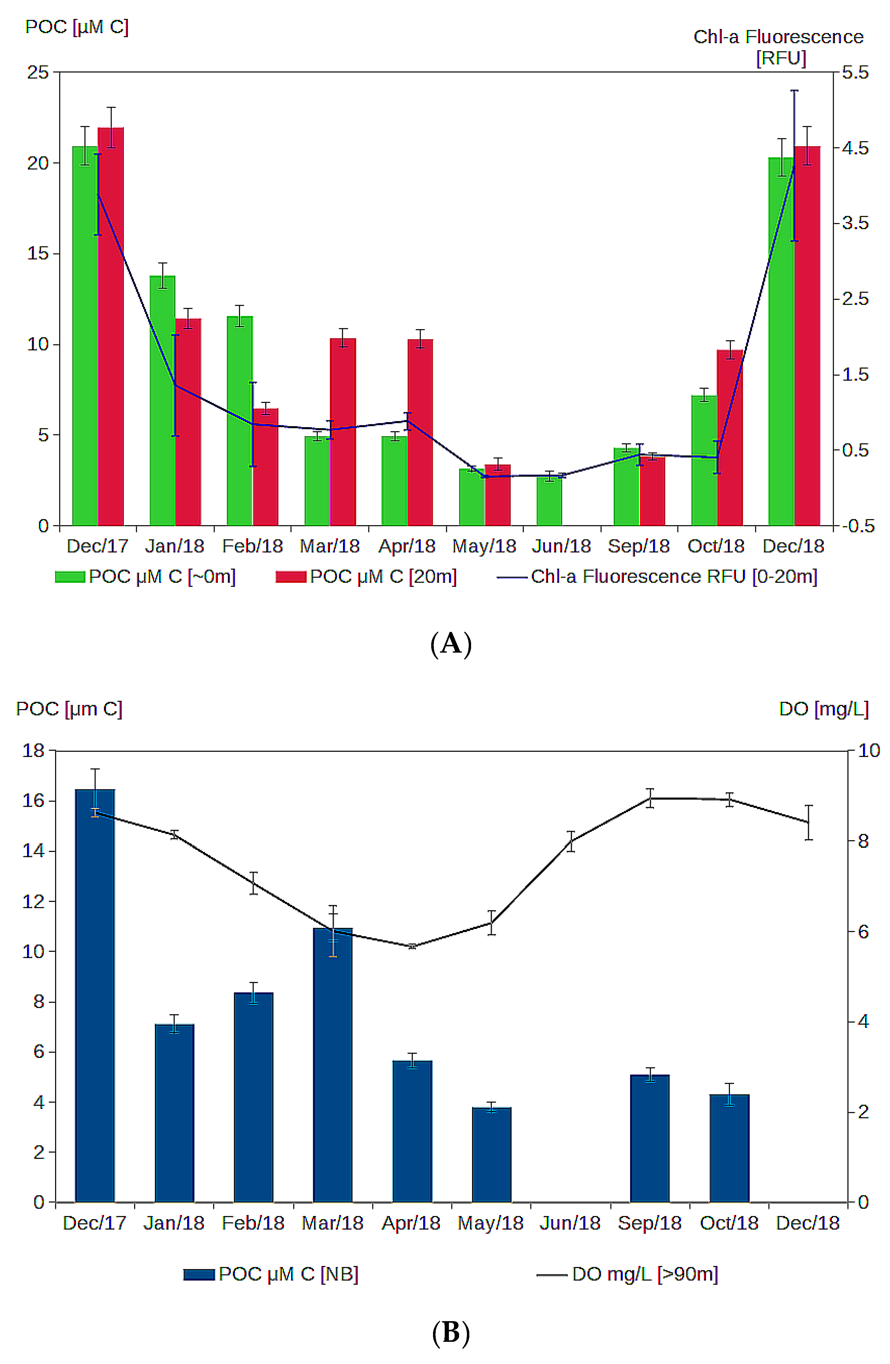
2.4. Particulate Organic Carbon Concentrations
2.5. Hydrodynamical Data
3. Results
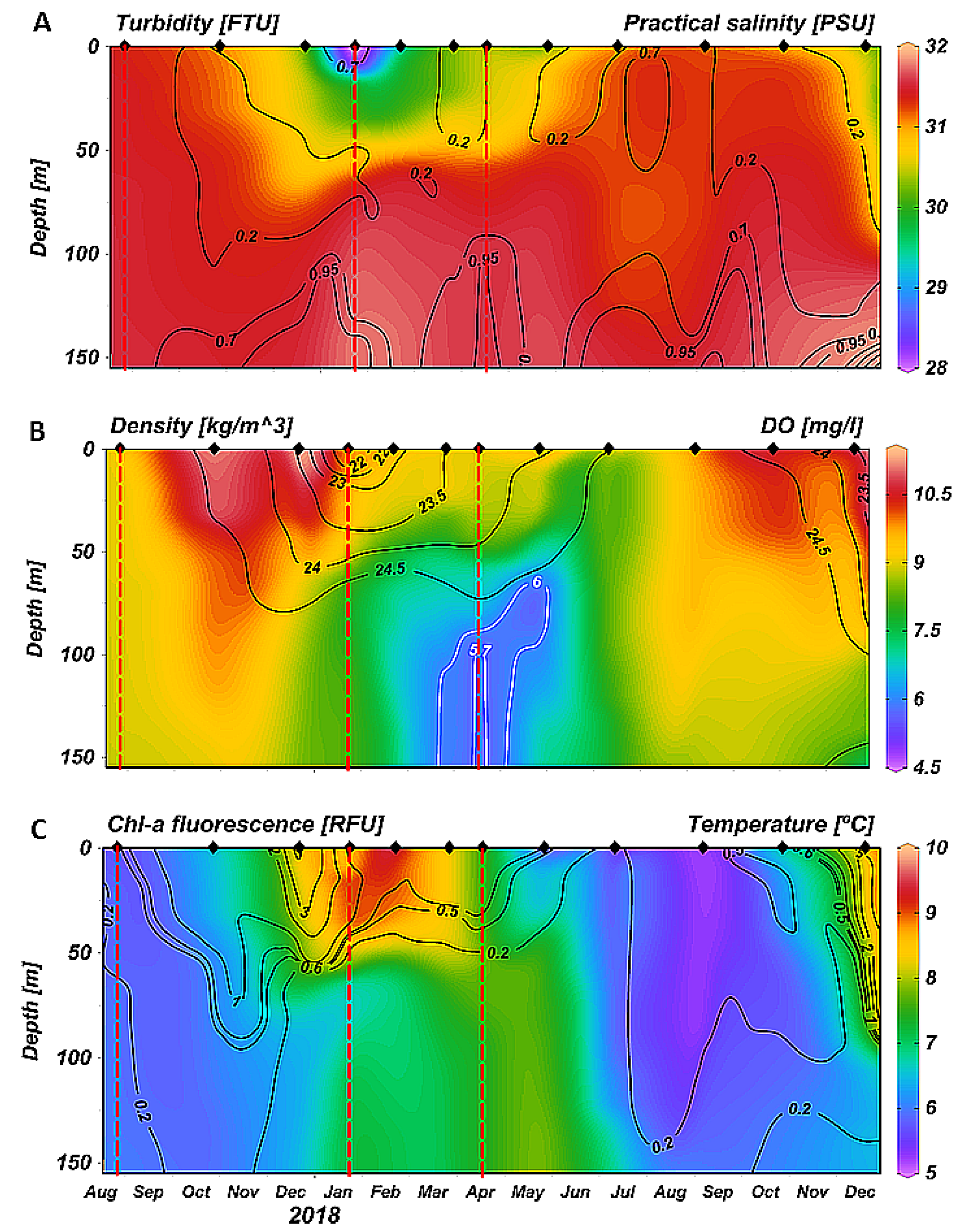
3.1. Temporal Variability of Hydrology: 2014–2018 Time Series at the Fixed Station
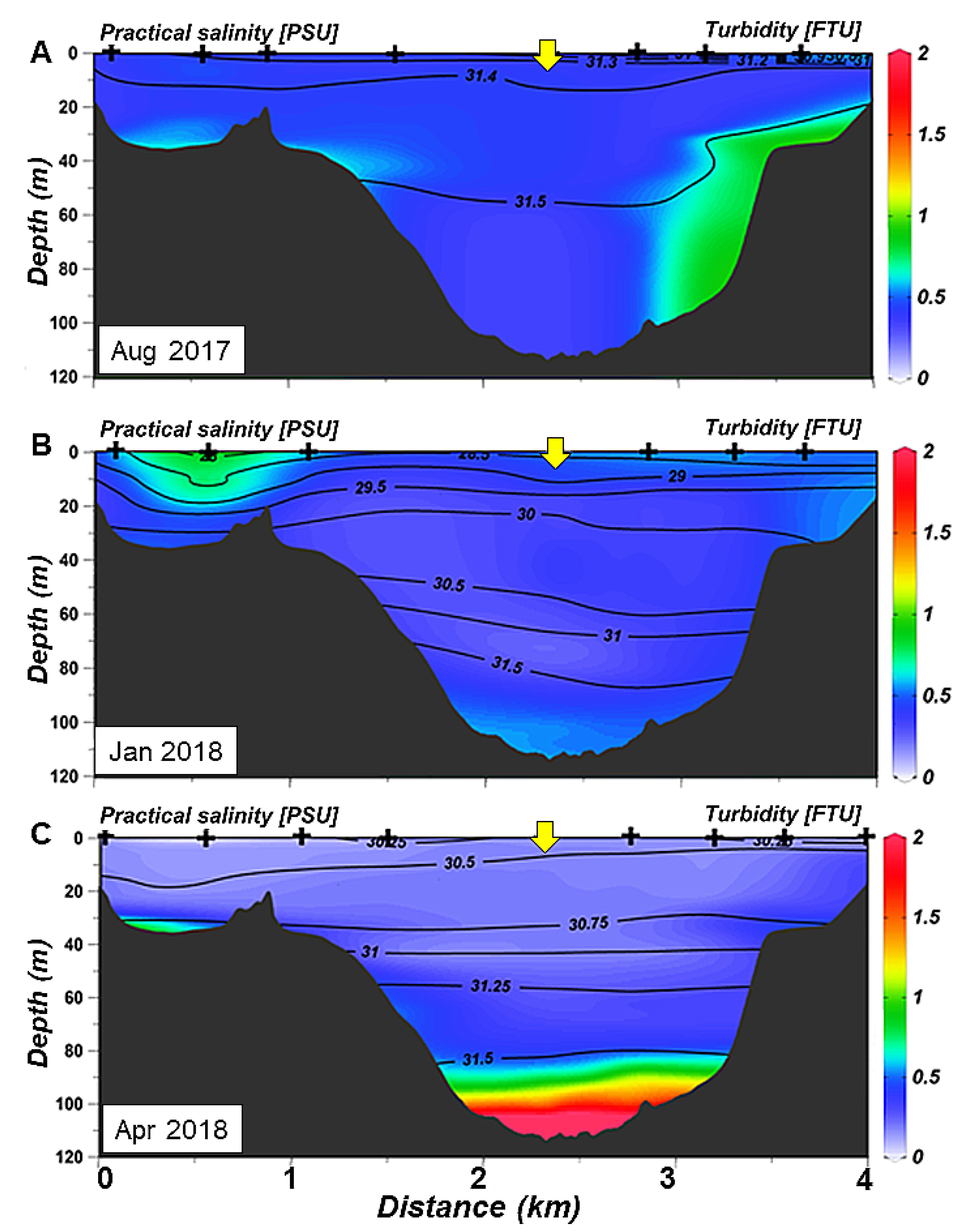
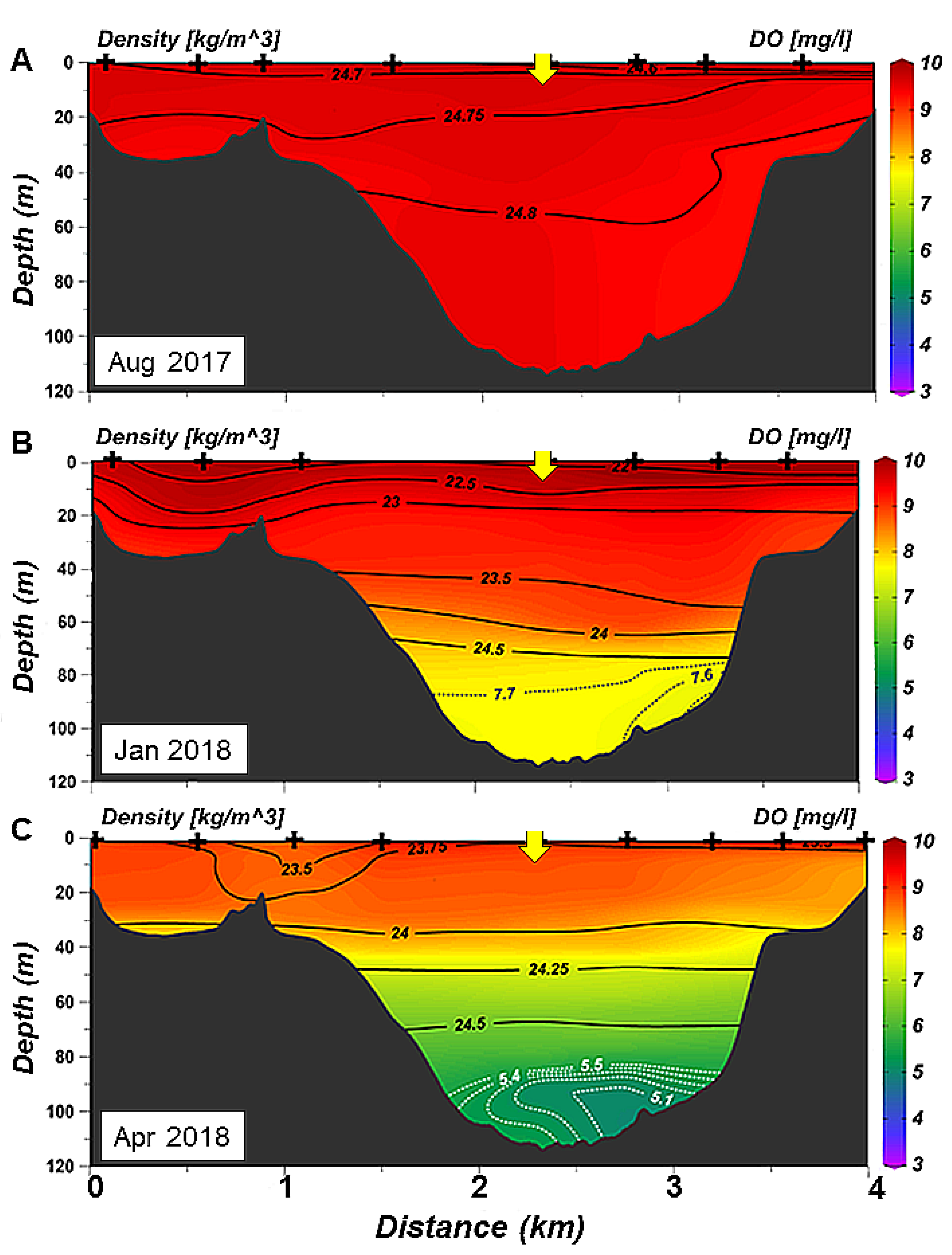
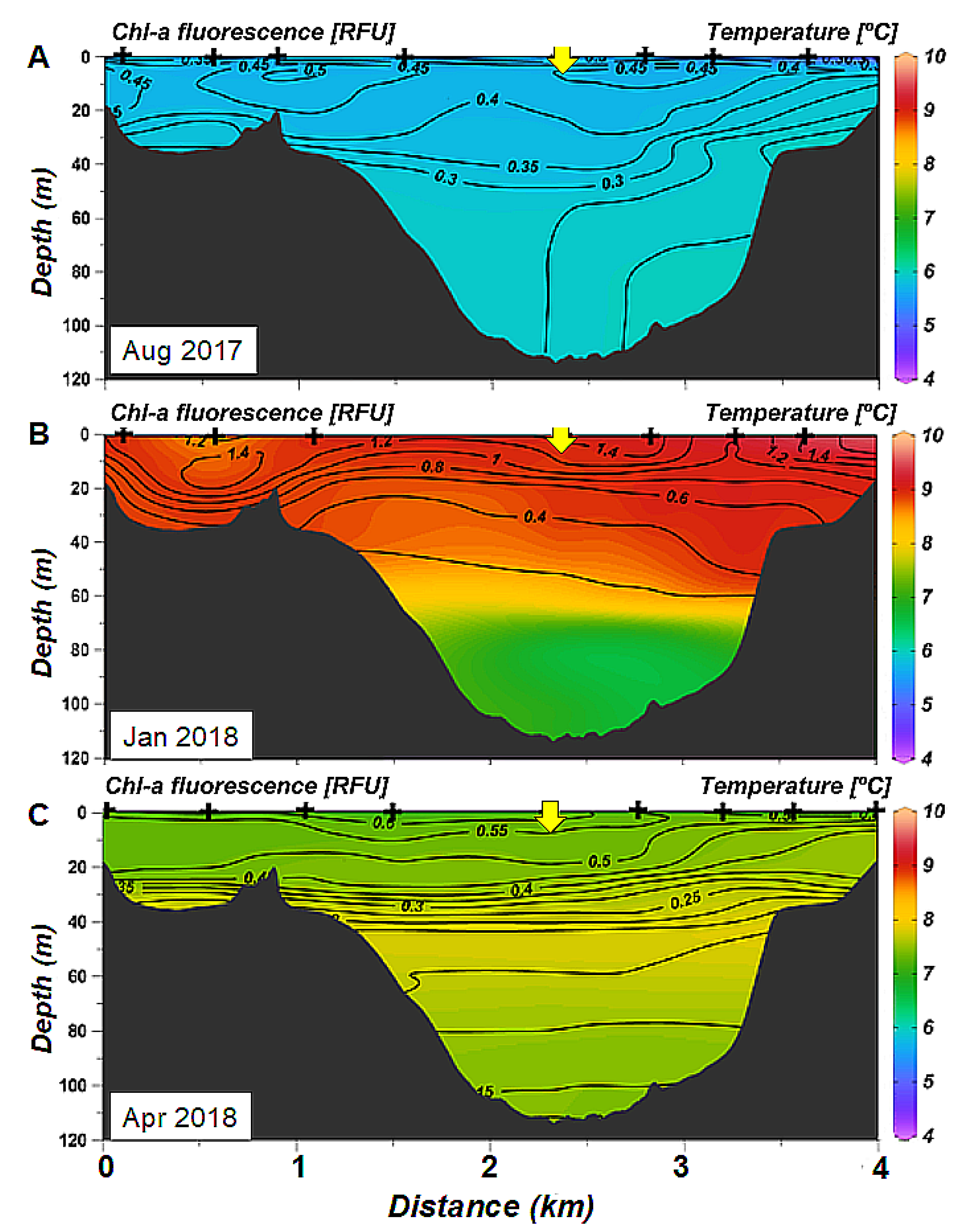
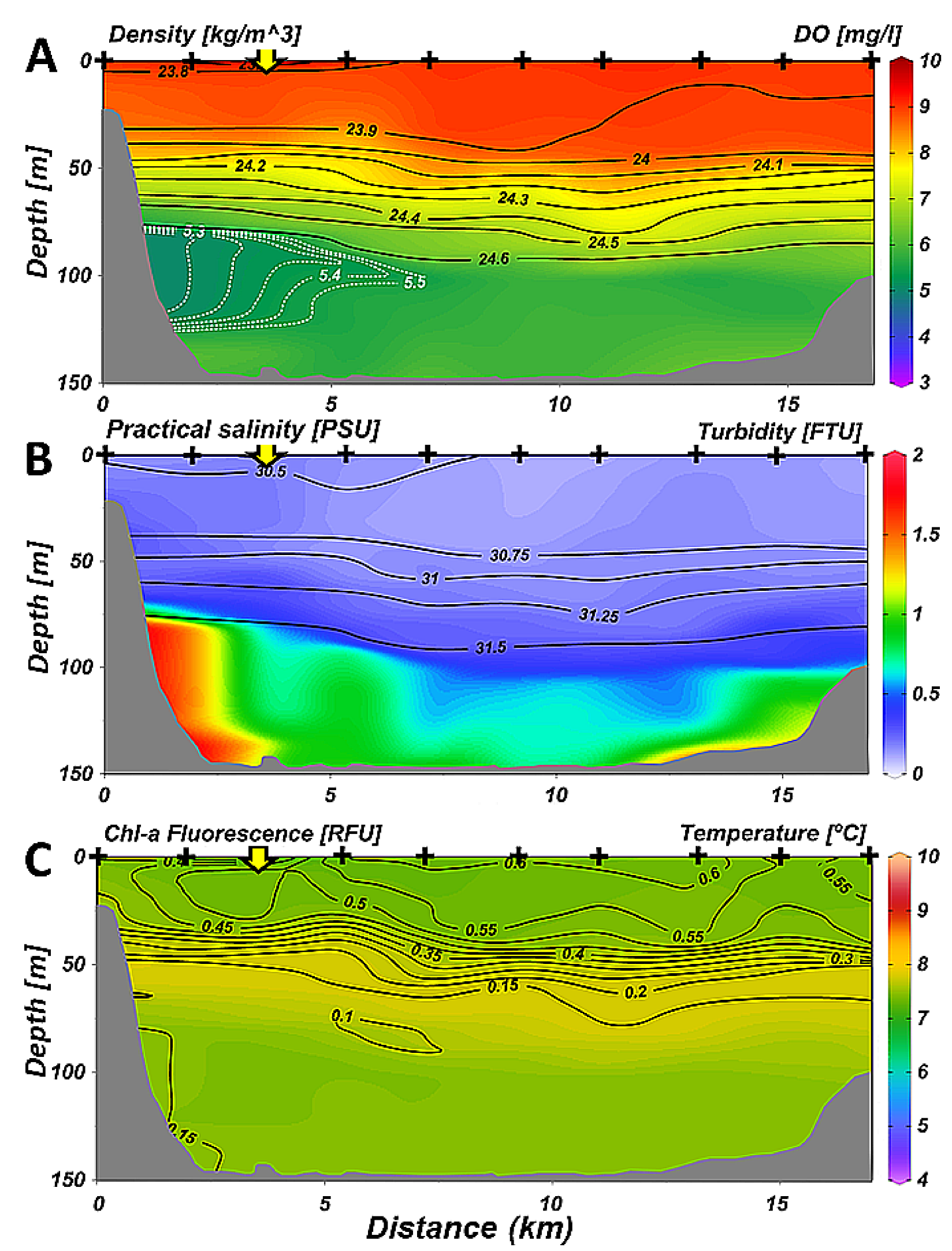
3.2. Spatial Variability of Hydrology: Seasonal Sections Across and Along the Ushuaia Bay and Valley
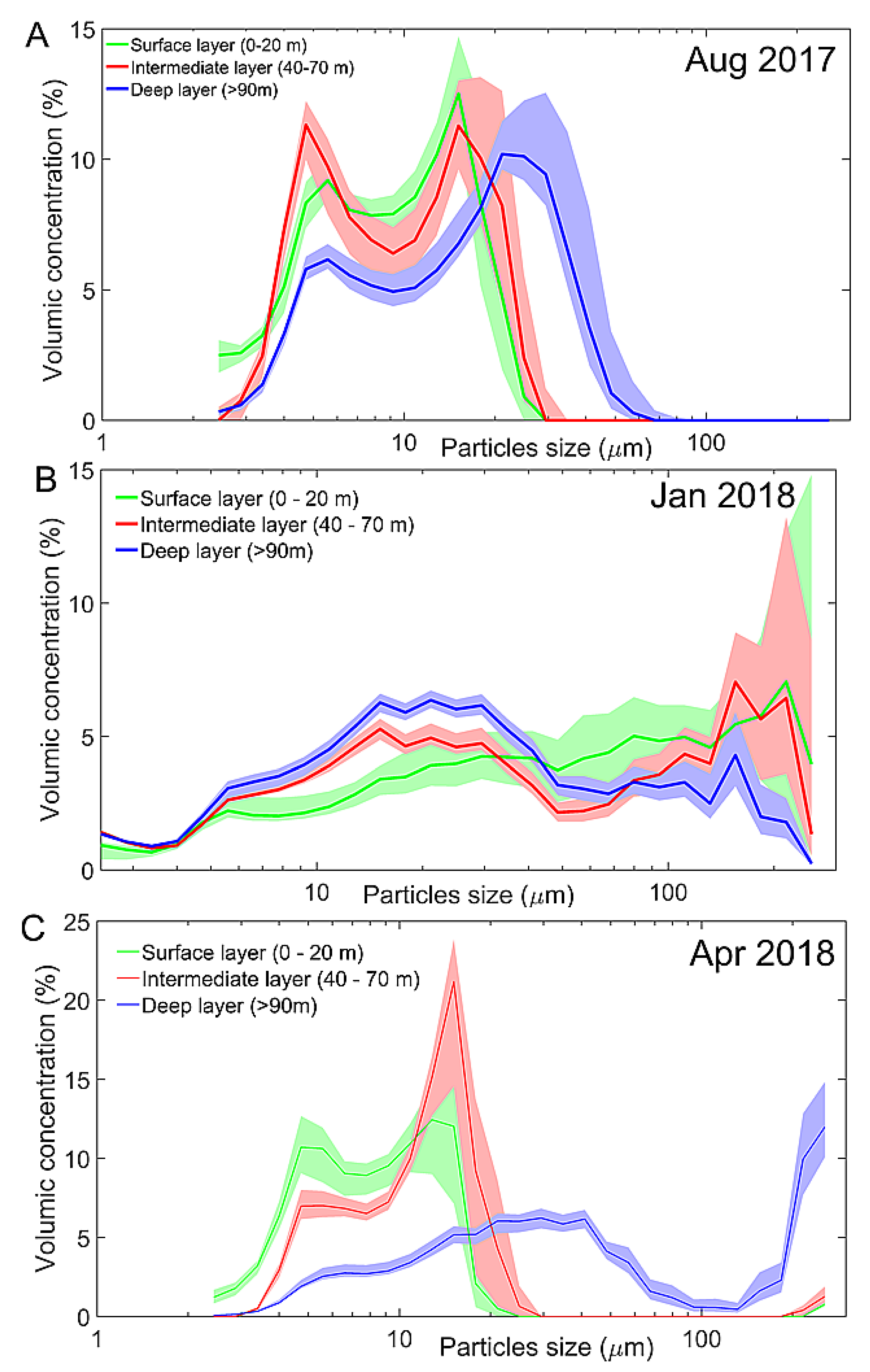
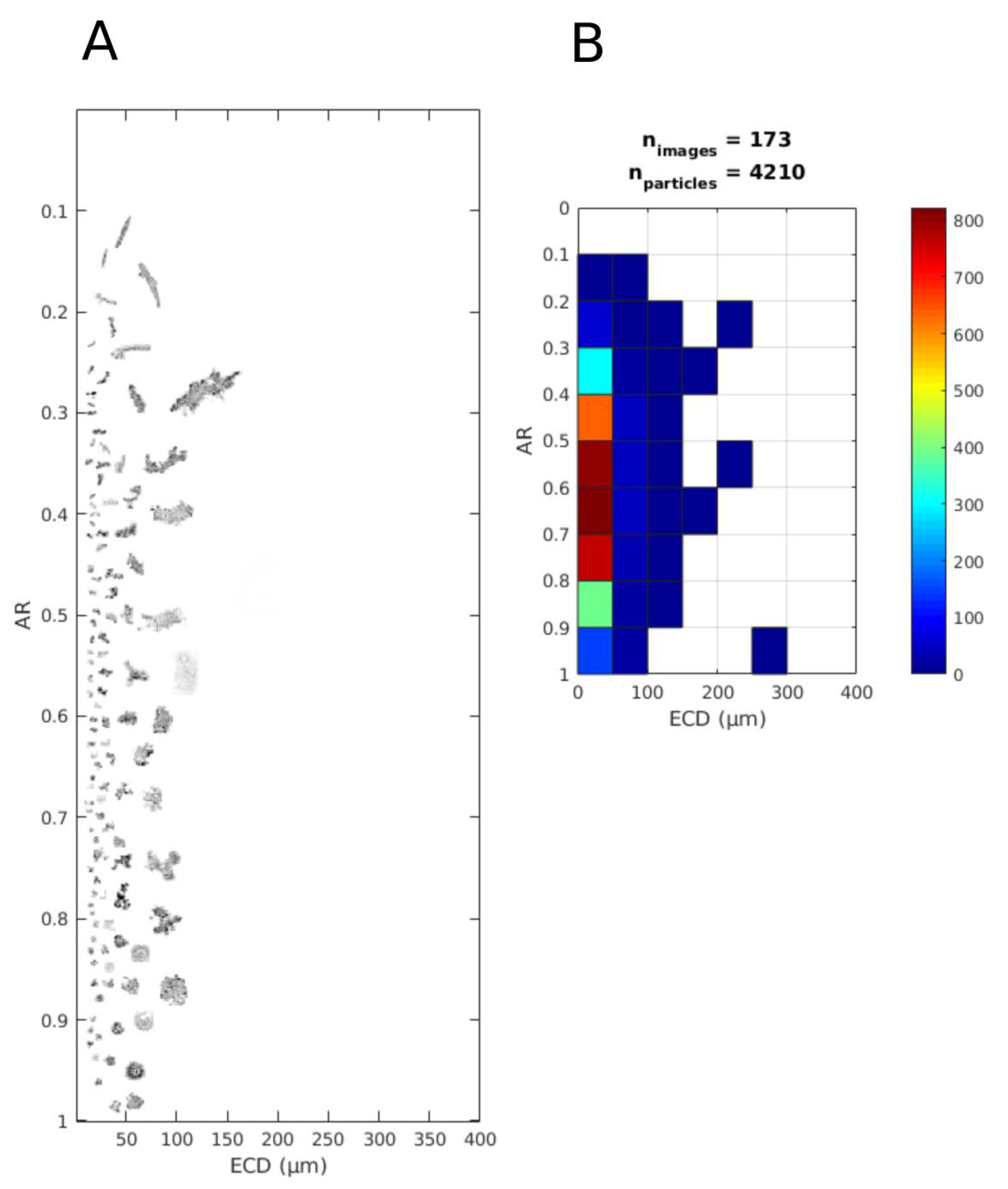
3.3. Particulate Matter Characteristics
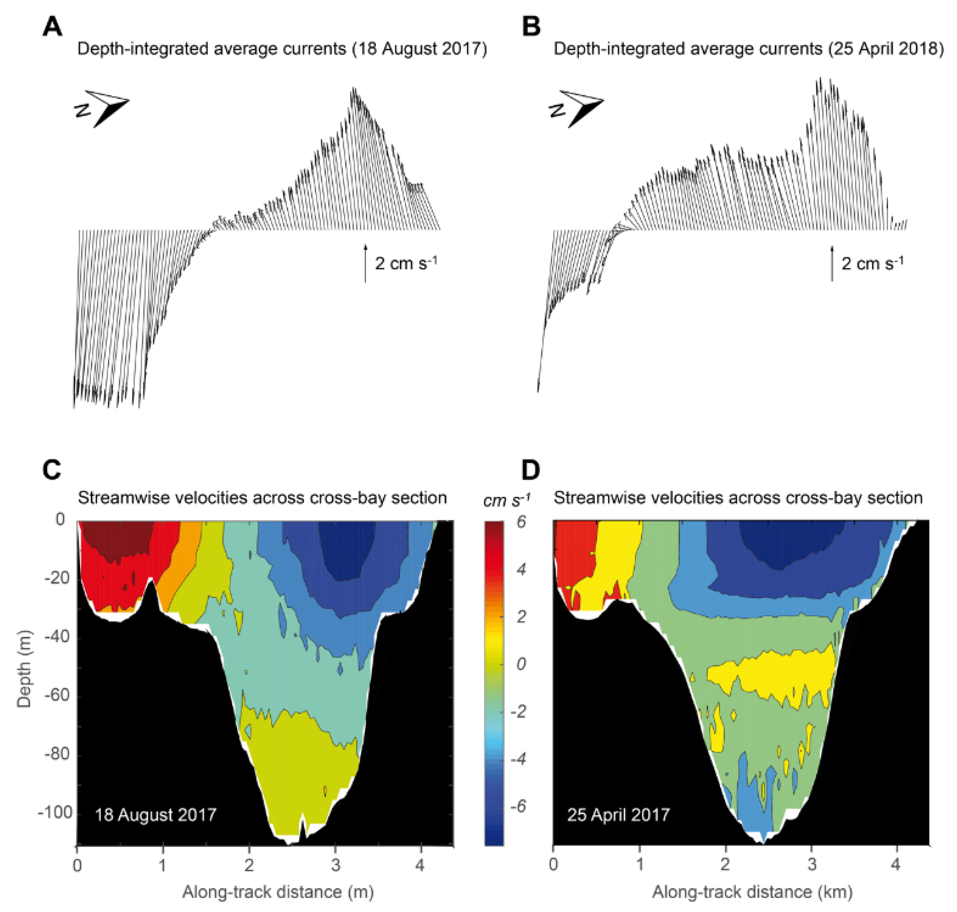
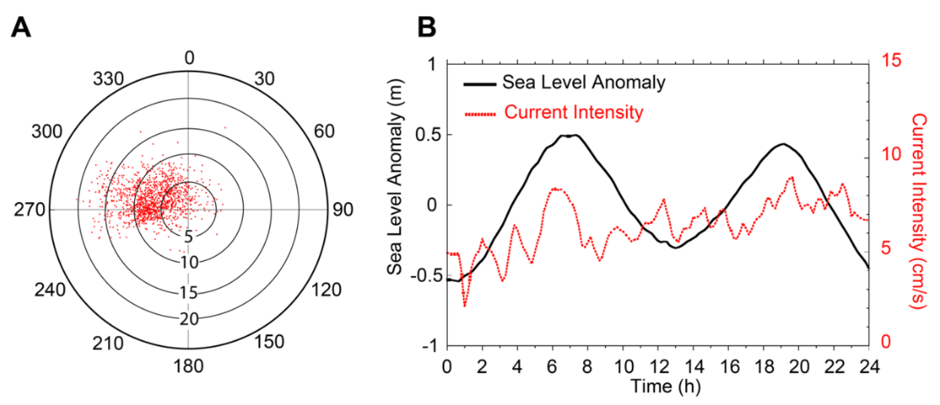
3.4. Currents Intensity and Variability
4. Discussion
5. Conclusions
- The seasonal stratification, observed during summer and autumn (December 2017–March2018), is induced mainly by freshwater inputs at the surface during snowmelt and is concomitance with planktonic production in the surface layer.
- Despite the inputs of organic matter of natural and urban origin by runoff, outside the most coastal part, the rest of Ushuaia Bay does not seem to be affected by these inputs because the rapid renewal of the bay’s waters maintains a high level of oxygenation.
- The decrease in oxygen in the deep layer in the proximal part of the valley during summer and autumn is likely due to the settling and degradation of planktonic organic matter produced in the surface layer, that is found in the form of aggregates in the deep layer and low water turnover.
- It is likely that a seasonal decrease in dissolved oxygen also occurs in the multiple deep sub-basins that are present along the Beagle Channel, due to deep layer stagnation and surface organic production in stratified periods.
- The DO depletion might extend in time and space in line with global warming, glacier retreat and the subsequent increase of vertical stratification, and thus yield to significant alterations of this sub-Antarctic ecosystem.
Author Contributions
Funding
Acknowledgments
Conflicts of Interest
References
- Wakeham, S.G.; Lee, C. Organic geochemistry of particulate matter in the ocean: The role of particles in oceanic sedimentary cycles. Org. Geochem. 1989, 14, 83–96. [Google Scholar] [CrossRef]
- Syvitski, J.P.M.; Burrell, D.C.; Skei, J.M. Fjords: Processes and Products; Springer Science & Business Media: New York, NY, USA, 1987; p. 379. [Google Scholar] [CrossRef]
- Zhang, J.; Gilbert, D.; Gooday, A.J.; Levin, L.; Naqvi, S.W.A.; Middelburg, J.J.; Van Der Plas, A.K. Natural and human-induced hypoxia and consequences for coastal areas: Synthesis and future development. Biogeosciences 2010, 7, 1443–1467. [Google Scholar] [CrossRef] [Green Version]
- Diaz, R.J.; Rosenberg, R. Marine benthic hypoxia: A review of its ecological effects and the behavioural responses of benthic macrofauna. Oceanogr. Mar. Biol. Annu. Rev. 1995, 33, 245–303. [Google Scholar]
- Vaquer-Sunyer, R.; Duarte, C.M. Thresholds of hypoxia for marine biodiversity. Proc. Natl. Acad. Sci. USA 2008, 105, 15452–15457. [Google Scholar] [CrossRef] [Green Version]
- Paschke, K.; Cumillaf, J.P.; Loyola, S.; Gebauer, P.; Urbina, M.; Chimal, M.E.; Rosas, C. Effect of dissolved oxygen level on respiratory metabolism, nutritional physiology, and immune condition of southern king crab Lithodes santolla (Molina, 1782) (Decapoda, Lithodidae). Mar. Biol. 2010, 157, 7–18. [Google Scholar] [CrossRef]
- Freeland, H.J.; Farmer, D.M.; Levings, C.D. Fjord Oceanography. In Proceedings of the NATO Conference on Fjord Oceanography, Victoria, BC, Canada, 4–8 June 1979; Plenum Press: New York, NY, USA; London, UK, 1980; p. 715. [Google Scholar]
- Isla, F.; Bujalesky, G.; Coronato, A. Procesos estuarinos en el canal Beagle, Tierra del Fuego Estuarine. Rev. Asoc. Geol. Argent. 1999, 54, 307–318. [Google Scholar]
- Bujalesky, G.; Aliotta, S.; Isla, F. Facies del subfondo del canal Beagle, Tierra del Fuego. Rev. Asoc. Geológica Argent. 2004, 59, 29–37. [Google Scholar]
- Iturraspe, R.J.; Sottini, R.; Schroeder, C.; Escobar, J. Hidrología y variables climáticas del Territorio de Tierra del Fuego. Información básica. Contrib. Científica CADIC 1989, 7, 196. [Google Scholar]
- Balestrini, C.; Manzella, G.; Lovrich, G.A. Simulación de corrientes en el Canal Beagle y Bahía Ushuaia, mediante un modelo bidimensional. Serv. Hidrogr. Nav. 1998, 98, 1–58. [Google Scholar]
- Bujalesky, G.G. The flood of the Beagle Valley (11,000 YR B.P.), Tierra del Fuego. An. Inst. Patagon. 2011, 39, 5–21. [Google Scholar] [CrossRef] [Green Version]
- Amin, O.; Comoglio, L.; Spetter, C.; Duarte, C.; Asteasuain, R.; Freije, R.H.; Marcovecchio, J. Assessment of land influence on a high-latitude marine coastal system: Tierra del Fuego, southernmost Argentina. Environ. Monit. Assess. 2011, 175, 63–73. [Google Scholar] [CrossRef]
- Torres, A.I.; Gil, M.N.; Amín, O.A.; Esteves, J.L. Environmental characterization of a eutrophicated semi-enclosed system: Nutrient budget (Encerrada Bay, Tierra del Fuego Island, Patagonia, Argentina). Water Air Soil Pollut. 2009, 204, 259–270. [Google Scholar] [CrossRef]
- Martín, J.; Colloca, C.; Diodato, S.; Malits, A. Variabilidad espacio-temporal de las concentraciones de oxígeno disuelto en Bahía Ushuaia y Canal Beagle (Tierra del Fuego). Nat. Patagónica 2016, 8, 193. [Google Scholar]
- Schlitzer, R. Ocean Data View. 2019. Available online: https://odv.awi.de (accessed on 28 October 2019).
- Agrawal, Y.C.; Pottsmith, H.C. Instruments for particle size and settling velocity ob-servations in sediment transport. Mar. Geol. 2000, 168, 89–114. [Google Scholar] [CrossRef]
- Agrawal, Y.C.; Whitmire, A.; Mikkelsen, O.A.; Pottsmith, H.C. Light scattering by random shaped particles and consequences on measuring suspended sediments by laser diffraction. J. Geophys. Res. 2008, 113. [Google Scholar] [CrossRef] [Green Version]
- Traykovski, P.; Latter, R.J.; Irish, J.D. A laboratory evaluation of the laser in situ scat-tering and transmissometery instrument using natural sediments. Mar. Geol. 1999, 159, 355–367. [Google Scholar] [CrossRef]
- Mikkelsen, O.A.; Hill, P.S.; Milligan, T.G.; Chant, R.J. In situ particle size distributions and volume concentrations from a LISST-100 laser particle sizer and a digital floc camera. Cont. Shelf Res. 2005, 25, 1959–1978. [Google Scholar] [CrossRef]
- Graham, G.W.; Smith, W.A.M. The application of holography to the analysis of size and settling velocity of suspended cohesive sediments. Limnol. Oceanogr. Methods 2010, 8, 1–15. [Google Scholar] [CrossRef]
- Aminot, A.; Kérouel, R. Hydrologie des Écosystèmes Marins: Paramètres et Analyses; Editions Quae; INRA: Versailles, France, 2004; p. 336. [Google Scholar]
- Balestrini, C.F.; Vinuesa, J.; Speroni, J.; Lovrich, G.; Mattenet, C.; Cantu, C.; Medina, P. Estudio de las Corrientes Marinas en los alrededores de la Península Ushuaia. Comun. Científica CADIC 1990, 10, 1–33. [Google Scholar]
- Schneider, W.; Pérez-Santos, I.; Ross, L.; Bravo, L.; Seguel, R.; Hernández, F. On the hydrography of Puyuhuapi Channel, Chilean Patagonia. Prog. Oceanogr. 2014, 129, 8–18. [Google Scholar] [CrossRef]
- Gil, M.N.; Torres, A.I.; Amin, O.; Esteves, J.L. Assessment of recent sediment influence in an urban polluted subantarctic coastal ecosystem. Beagle Channel (Southern Argentina). Mar. Pollut. Bull. 2011, 62, 201–207. [Google Scholar] [CrossRef] [PubMed]
- Björk, G.; Nordberg, K.; Arneborg, L.; Bornmalm, L.; Harland, R.; Robijn, A.; Ödalen, M. Seasonal oxygen depletion in a shallow sill fjord on the Swedish west coast. J. Mar. Syst. 2017, 175, 1–14. [Google Scholar] [CrossRef]
- Caballero-Alfonso, A.M.; Carstensen, J.; Conley, D.J. Biogeochemical and environmental drivers of coastal hypoxia. J. Mar. Syst. 2015, 141, 190–199. [Google Scholar] [CrossRef] [Green Version]
- Breitburg, D.; Levin, L.A.; Oschlies, A.; Grégoire, M.; Chavez, F.P.; Conley, D.J.; Zhang, J. Declining oxygen in the global ocean and coastal waters. Science 2018, 359. [Google Scholar] [CrossRef] [Green Version]
- Thomas, Y.; Flye-Sainte-Marie, J.; Chabot, D.; Aguirre-Velarde, A.; Marques, G.M.; Pecquerie, L. Effects of hypoxia on metabolic functions in marine organisms: Observed patterns and modeling assumptions within the context of Dynamic Energy Budget (DEB) theory. J. Sea Res. 2019, 143, 231–242. [Google Scholar] [CrossRef] [Green Version]
- Lovrich, G.A.; Tapella, F.; Di Salvatore, P.; Gowland-Sainz, M.F.; Diez, M.J.; Fernández, A.L.; Sotelano, M.P.; Romero, M.C.; Negri, M.F.; Chiesa, I.; et al. Estado poblacional de la centolla Lithodes santolla en el Canal Beagle—2016—Cluster de Pesca Artesanal de Tierra del Fuego. In Cluster de Pesca Artesanal de Tierra del Fuego Convenio Específico de Asistencia Técnica CONICET-UNTDF (Res 361/15); Researchgate: Ushuaia, Argentina, 2017; p. 85. [Google Scholar] [CrossRef]
- Tapella, F.; Lovrich, G.A. Asentamiento de estadios tempranos de las centollas Lithodes santolla y Paralomis granulosa (Decapoda: Lithodidae) en colectores artificiales pasivos en el Canal Beagle, Argentina. Investig. Mar. 2006, 34, 47–55. [Google Scholar] [CrossRef] [Green Version]
- Urbina, M.A.; Paschke, K.; Gebauer, P.; Cumillaf, J.P.; Rosas, C. Physiological responses of the southern king crab, Lithodes santolla (Decapoda: Lithodidae), to aerial exposure. Comp. Biochem. Physiol. Part A Mol. Integr. Physiol. 2013, 166, 538–545. [Google Scholar] [CrossRef]


| Parameter | Instrument | Period | |||
|---|---|---|---|---|---|
| August 2017 December 2018 | August 2017 | January 2018 | April 2018 | ||
| Temperature, Salinity, Density, Oxygen, Turbidity, Fluorescence | CTD | Fixed station | Cross Bay (B1–B8) | Cross Bay (B1–B8) | Cross Bay (B1–B9) Along Bay (A1–A10) |
| Particle size spectra | LISST-100X | - | Cross Bay (B1–B8) | Cross Bay (B1–B8) | Cross Bay (B1–B9) |
| Particle images | LISST-Holo | - | Cross Bay (B1–B8) | - | - |
| Currents | ADCP | - | Cross Bay (B1–B8) | - | Cross Bay (B1–B9) |
| POC | Niskin bottle | Fixed station (*) | - | - | - |
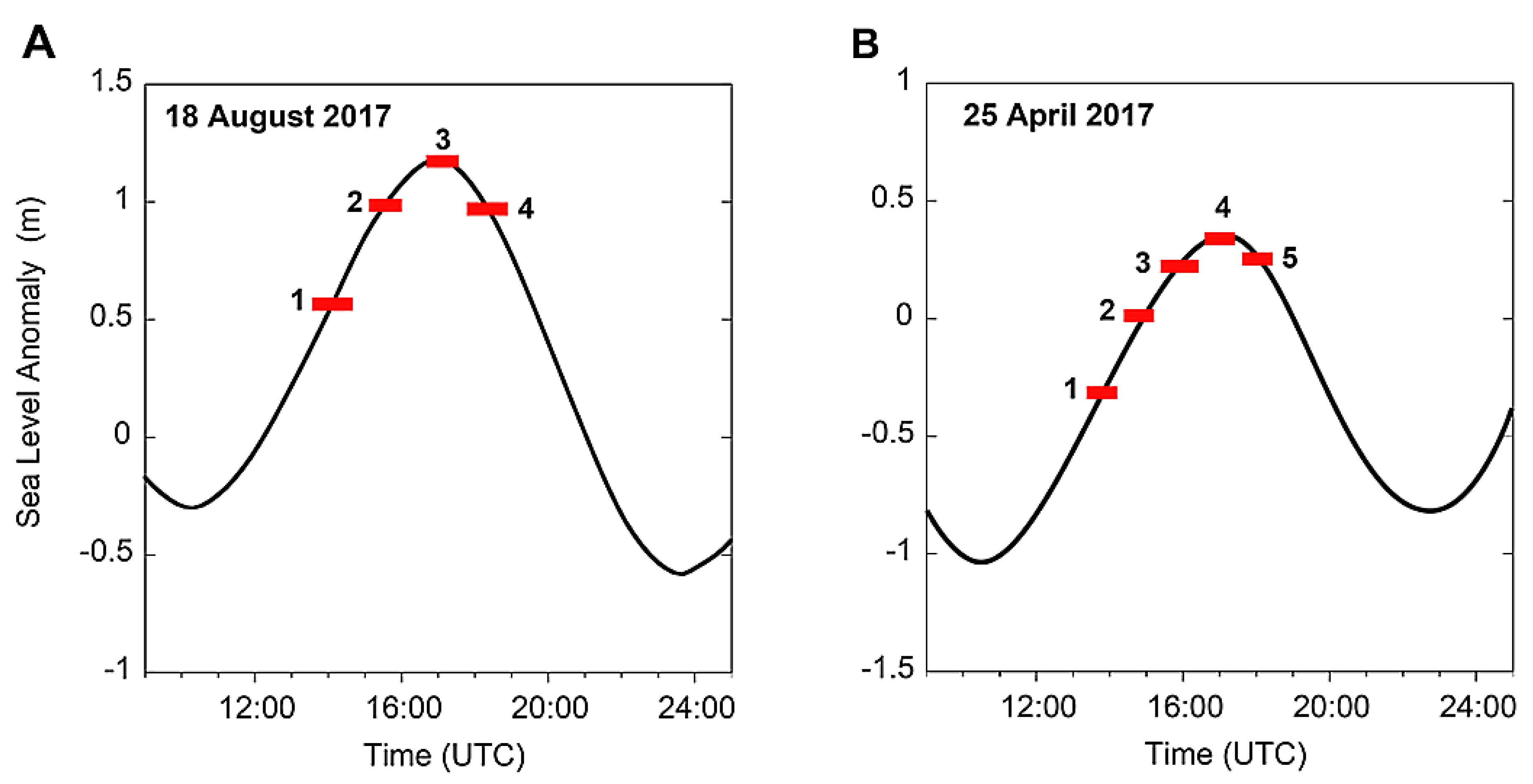
| 18 August 2017 | 25 April 2018 |
|---|---|
| 13:19–14:10 UTC | |
| Flood: High Tide − 3 h 00 | |
| Inflow: 4.5 × 10³ m3/s | |
| 14:10–14:40 UTC | 14:33–15:13 UTC |
| Flood: High Tide − 2 h 00 | Flood: High Tide − 2 h 00 |
| Inflow: 3.3 × 10³ m3/s | Inflow: 4.7 × 10³ m3/s |
| 15:11–15:59 UTC | 15:33–16:18 UTC |
| Flood: High Tide − 1 h 00 | Flood: High Tide − 1 h 00 |
| Inflow: 4.1 × 10³ m3/s | Inflow: 5.2 × 10³ m3/s |
| 16:44–17:30 UTC | 16:43–17:19 UTC |
| Slack water: High Tide | Slack water: High Tide |
| Inflow: 3.2 × 10³ m3/s | Inflow: 3.50 × 10³ m3/s |
| 17:58–18:46 UTC | 17:41–18:21 UTC |
| Ebb: High Tide + 1 h 00 | Ebb: High Tide + 1 h 00 |
| Inflow: 3.1 × 10³ m3/s | Inflow: 2.6 × 10³ m3/s |
© 2020 by the authors. Licensee MDPI, Basel, Switzerland. This article is an open access article distributed under the terms and conditions of the Creative Commons Attribution (CC BY) license (http://creativecommons.org/licenses/by/4.0/).
Share and Cite
Flores Melo, X.; Martín, J.; Kerdel, L.; Bourrin, F.; Colloca, C.B.; Menniti, C.; de Madron, X.D. Particle Dynamics in Ushuaia Bay (Tierra del Fuego)-Potential Effect on Dissolved Oxygen Depletion. Water 2020, 12, 324. https://doi.org/10.3390/w12020324
Flores Melo X, Martín J, Kerdel L, Bourrin F, Colloca CB, Menniti C, de Madron XD. Particle Dynamics in Ushuaia Bay (Tierra del Fuego)-Potential Effect on Dissolved Oxygen Depletion. Water. 2020; 12(2):324. https://doi.org/10.3390/w12020324
Chicago/Turabian StyleFlores Melo, Ximena, Jacobo Martín, Lounes Kerdel, François Bourrin, Cristina Beatriz Colloca, Christophe Menniti, and Xavier Durrieu de Madron. 2020. "Particle Dynamics in Ushuaia Bay (Tierra del Fuego)-Potential Effect on Dissolved Oxygen Depletion" Water 12, no. 2: 324. https://doi.org/10.3390/w12020324