Characterization of Diffuse Groundwater Inflows into Streamwater (Part I: Spatial and Temporal Mapping Framework Based on Fiber Optic Distributed Temperature Sensing)

Abstract

Although fiber optic distributed temperature sensing (FO-DTS) has been used in hydrology for the past 10 years to characterize groundwater–streamwater exchanges, it has not been widely applied since the entire annual hydrological cycle has rarely been considered. Properly distinguishing between diffuse and intermittent groundwater inflows requires longer periods (e.g., a few months, 1 year) since punctual changes can be lost over shorter periods. In this study, we collected a large amount of data over a one-year period using a 614 m long cable placed in a stream. We used a framework based on a set of hypotheses approach using thermal contrast between stream temperature and the atmosphere. For each subreach, thermal contrast was normalized using reference points assumed to lie outside of groundwater influence. The concepts and relations developed in this study provide a useful and simple methodology to analyze a large database of stream temperature at high spatial and temporal resolution over a one-year period using FO-DTS. Thus, the study highlighted the importance of streambed topography, since riffles and perched reaches had many fewer inflows than pools. Additionally, the spatial extent of groundwater inflows increased at some locations during high flow. The results were compared to the usual standard deviation of stream temperature calculated over an entire year. The two methods located the same inflows but differed in the mapping of their spatial extent. The temperatures obtained from FO-DTS open perspectives to understand spatial and temporal changes in interactions between groundwater and surface water.

1. Introduction

Groundwater inflows into streams play an important role in the ecological balance of streams, contributing chemicals that drive water quality [1,2,3,4,5], supporting baseflow [6,7,8,9,10,11] and providing refuge for fauna [12,13,14,15,16,17,18,19,20,21]. Locating and mapping inflows is thus of great interest for river management and ecological restoration [22,23,24,25,26]. However, groundwater inflows are usually driven by multiple factors, including hydraulic head gradients between streamwater and groundwater, stream geomorphology, and subsurface geology [27,28,29]. Multiscale processes involved in groundwater and streamwater exchange can be categorized as large- or small-scale [30]. Large-scale hydrological exchange is driven mainly by the spatial and temporal hydraulic head gradients between the stream and the surrounding groundwater. By contrast, at a small-scale, water is pushed into the streambed due to interaction between the flow and morphological features of the streambed such as riffle–pool sequences. Variability in hydraulic conductivity influences both large- and small-scale processes [31,32,33]. The spatial distribution of geological heterogeneities influences stream–groundwater exchange [34,35]. Using a two-dimensional groundwater flow model to investigate the interface between the stream and groundwater hyporheic (below stream) zone, Wroblicky et al. [36] identified hydraulic conductivity of alluvial and streambed sediments as a major factor controlling stream–groundwater exchange. Mojarrad et al. [37] quantified effects of catchment-scale upwelling groundwater on hyporheic fluxes and tested a wide range of spatial scales. Their results identified streambed topographic structures as the predominant factor controlling the magnitude of hyporheic exchange fluxes. Predicting groundwater flow paths from groundwater–surface water analysis of easily available data, such as temperature, helps to identify catchment behaviors. Because groundwater inflows are heterogeneous in space and variable in time, locating and mapping them is challenging.

Many methods can be used to map groundwater inflow zones in rivers [38]. Some methods use a direct approach, such as measuring discharge in successive cross sections (i.e., differential gauging) to determine gains and losses along a reach. Others use natural markers of inflow such as specific biological communities [39,40,41]. Most, however, usually use tracers. For instance, many studies monitored radon concentrations or stable-isotope ratios to detect groundwater inflows to rivers [42,43,44,45,46]. Among other possible tracers (e.g., ions, contaminants), heat has been recognized as reliable for identifying exchanges between groundwater and surface water [47,48,49]. Most methods using heat as a tracer are based on punctual temperature measurements [50]. Such standard measurement techniques are usually based on placing temperature sensors directly into the water column [51], in a streambed piezometer or along thermal lances into shallow sediments [52]. However, all have a limited spatial range that does not allow the heterogeneity of groundwater–stream interactions, nor their possible temporal intermittency, to be mapped at sufficient resolution. Only the recent development of airborne thermal infrared imagery (TIR) [30,53] and fiber optic distributed temperature sensing (FO-DTS) has provided good spatial coverage of stream thermal heterogeneities. TIR is an indirect technique that measures the temperature of the stream surface only [54,55]. It has a larger spatial range than FO-DTS, but lower accuracy and temporal resolution [56].

FO-DTS sensors send a laser impulse down a fiber optic cable to infer temperature along the cable. The measured ratio of the temperature-dependent Raman backscattered signal (anti-Stokes) to the temperature-independent Raman signal (Stokes) provides the temperature, while the time required for the backscattered signal to return provides the temperature’s location. This technique provides direct measurements every 0.25 m along a cable a few km long, with an accuracy as high as 0.05 °C depending on the brand, setup, and chosen configuration [57,58]. The spatial resolution and accuracy of FO-DTS can be used to map groundwater inflows, which are more thermally stable over time than streamwater. Indeed, stream temperature is usually influenced more by air temperature [59,60,61]; however where groundwater inflows, however, the stream temperature varies less over time. Calculating a simple standard deviation (SD) of temperature for a given period (from hours to years) and location is usually sufficient to identify stream points influenced by groundwater inflows (low SD) from points that are not (higher SD) [62]. However, this method can be problematic for intermittent inflows such as those during short high-water episodes, droughts, and floods. The time period over which thermal variability is calculated can obviously be adapted to address these episodes, but the approach still requires a long period of observations to properly distinguish groundwater from hyporheic recirculation [63]. Thus, potential changes in groundwater inflow dynamics could be hidden by transitional periods (e.g., beginning of high flows).

The present study applied a simple framework to a new study site to identify and interpret groundwater–surface water interactions. The framework maps groundwater inflows at individual timesteps using the thermal contrast between FO-DTS measurements in the hyporheic zone and the atmosphere. This framework thus attempts to characterize the spatiotemporal heterogeneity of groundwater inflows. After describing the testing of our framework in a second-order stream, we discuss its potentials and limits.

2. Materials and Methods

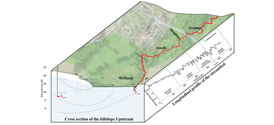
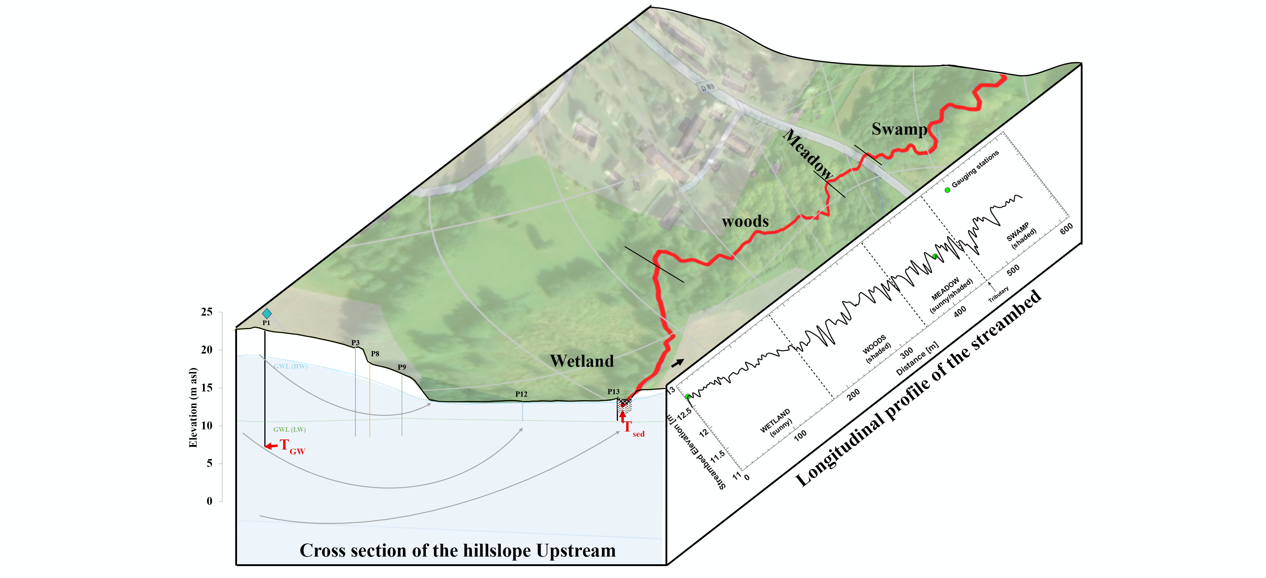
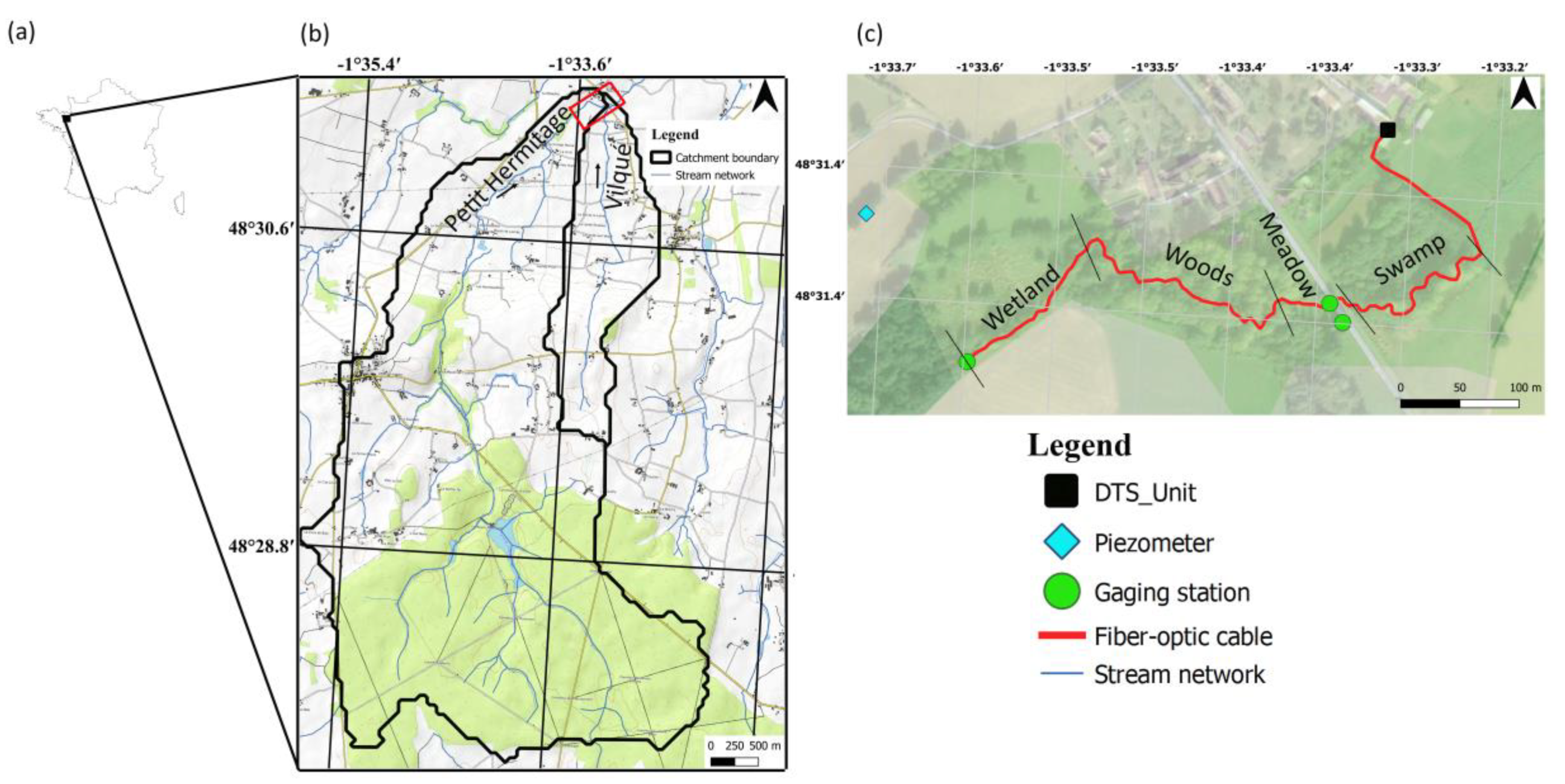
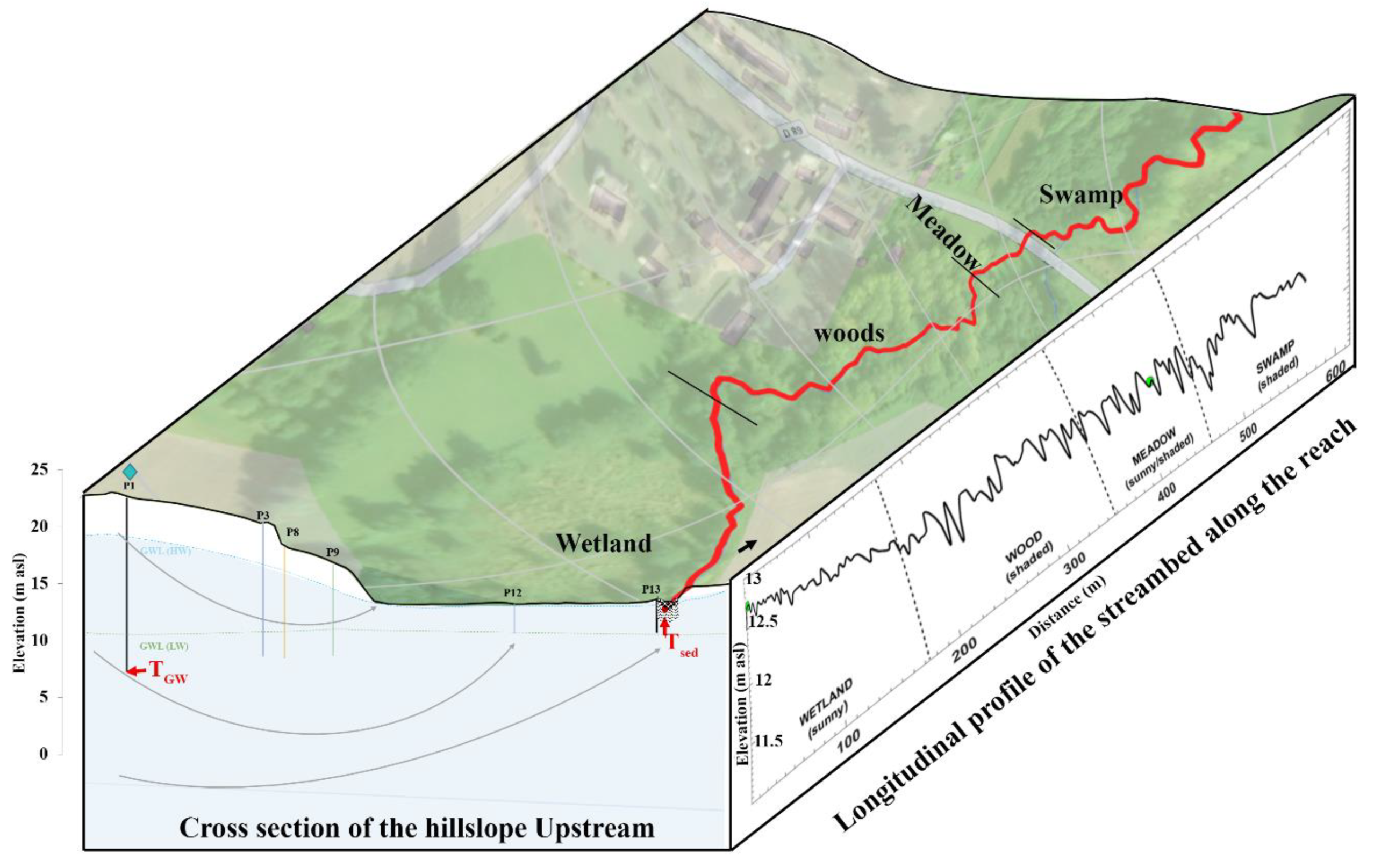
2.1. Study Site

We performed our study in an area in northeastern Brittany, France, called the Zone Atelier Armorique (ZAAr). The ZAAr is part of the International Long-Term Socio-Ecological Research Network LTSER (www.lter-europe.net). We collected a large amount of temperature data at high spatial and temporal resolutions. Measurements were made along a 614 m long reach of the Petit Hermitage, a second-order stream [64] that drains a 16 km² subwatershed and flows from south to north. The monitored reach represents the last several hundred meters of the Petit Hermitage were monitored until its confluence with its last tributary, the Vilqué (Figure 1c), which is a first-order stream draining an adjacent 2.34 km² watershed with a similar flow direction. The northern part of the ZAAr, where the monitoring occurred, lies on schist bedrock and loess. The southern part of the ZAAr, where the Petit Hermitage has its source, lies on granodiorite and altered hornfels. The bedrock of the entire area is overlain by a weathered zone considered to be the main unconfined aquifer of the area [65,66]. Soil and land-use characteristics reflect this north–south dichotomy: upstream soils (south) are characterized by a mix of silica sand and altered schist with forests. Downstream soils (north, monitored reach) are mainly aeolian and alluvial silts with wetlands, agricultural fields, and meadows. The streambed is thus a mix of silt and deposited organic matter, with sand coming from upstream. The climate in the region is oceanic, with mean annual precipitation of 965 mm and air temperatures generally ranging from 0 to 25 °C, with some exceptional events below 0 °C or above 30 °C. Rainfall and temperature data for the site were obtained from a weather station 1 km north (downstream) of the reach.

Previous studies offered good insight into the area [67,68] since results of long-term measurements were already available (e.g., soil moisture, piezometers, weather station, water quality, stream discharge, thermal dataloggers). In addition, the site was susceptible to dispersed groundwater inflows [69] and highly stratified reactivity [70], likely related to the high geological heterogeneities. The upstream monitored reach consists of a heavily monitored hillslope including a large wetland (Figure 1). The middle area is dominated by small woods followed by a meadow. The confluence is located in a woody wetland (hereafter, “swamp”). From this land-use typology, four subreaches were defined: wetland, woods, meadow, and swamp. Previous studies found the Vilqué tributary strongly influenced by groundwater throughout the year, although it was not accessible for direct measurements.

The longitudinal elevation of the Petit Hermitage streambed was measured with a theodolite (Leica) ca. every 4 m. The wetland, the most upstream subreach of the main stream, varies little in elevation, with small pools a few cm deep (Figure 2). However, the wetland has a steeper overall slope (ca. 2.4‰) than the rest of the stream (0.08‰) because a former deviation of the stream during the 19th century and the 1950s created a perched streambed in this reach (Figure 2). Despite high banks (ca. 50–80 cm above the streambed) and many bulrushes, it is sunnier than the following subreaches. The woods, with willows and bushes, are much more forested. It is also a wetland, but with more pronounced meandering and a clear succession of riffles and deep pools (every 40–50 cm). The following meadow subreach is straighter, with its left bank occupied by sheep. It is partly shaded because of bushes on the right bank, a narrower streambed and trees in its last third, but sunlight can still hit the stream surface at noon or in summer in some locations. A road bridge crosses over the stream in its last third. The swamp is the last subreach of the stream, which begins immediately after the confluence with the Vilqué tributary. It is similar to the woods but has smaller woody vegetation, more pronounced meanders and larger (although fewer) pools. Its banks (40 cm above the streambed) are also slightly lower than those of upstream subreaches (50–80 cm), so groundwater outcrops during high-water periods, and the soil remains wet most of the year. The most downstream part of this subreach was not accessible during the topography campaign due to fallen trees; thus, elevation data covered a shorter distance than the 614 m long thermal data from the FO-DTS cable.

2.2. Piezometry and Differential Gauging

Large-scale groundwater movements and periods of potential stream loss and/or gain [71] were determined using the pre-existing network of piezometers and gauging stations (Figure 1). The depth of these piezometers varies from 15 m on the hillslope to 4.5 m near the stream in the wetland. Groundwater level was monitored by a minidiver submersible pressure transducer (HOBO Pro v2), with an accuracy of ±0.2 cm and a 5 min timestep. Only the 15 m deep piezometer, located on the crest of the hillslope, was used in this study (Figure 1 and Figure 2a) to simplify interpretation by providing only the general hydraulic gradient with the stream. Streamwater stages were monitored using OTT Opheus sensors, with identical accuracy (±0.5 cm) and timestep (5 min), at two gauging stations (Figure 1 and Figure 2). Discharge was measured at each gauging station ca. every two months using the salt dilution method [72]. The resulting discharges were used to refine pre-existing rating curves and thus infer stream discharge time series based on water level measurements at each gauging station. These discharges (L s⁻¹) were converted into specific flow rates Qs (L s⁻¹ km⁻²) by dividing them by their respective drained areas. These specific discharges were used to compare the relative groundwater contribution over time at these points. Groundwater and streamwater levels were expressed in m above sea level (m asl) for comparison purposes.

2.3. Temperature Measurements

Locations of groundwater inflows in the stream were collected using a distributed temperature sensor (Ultima XT-DTS, Silixa Ltd, London, UK) with a dual-ended duplexed configuration [73], 40 min time integration and 0.25 m spatial sampling. The fiber optic cable was a 4 mm wide Brussens cable (Brugg, Switzerland) protected by stainless steel armoring and polyamide. Short segments of the cable (20–30 m) were coiled in two water baths for calibration [57]. A cold bath inside a refrigerator and a heated and insulated warm bath were kept thermally homogeneous with bubblers and monitored with RBRsolo temperature loggers with an accuracy of 0.002 °C. The FO-DTS system was calibrated following van de Giesen et al. [73] using the reference temperatures in the baths. Due to a lack of electricity at the end of the cable, no validation bath could be set up. Temperature measurement of the FO-DTS system and a thermal lance (Umwelt-und Ingenieurtechnik GmbH, Germany) were compared to assess measurement accuracy broadly. The FO-DTS cable near the lance was found uncovered by sediment most of the year, so the instruments were compared with the lance set in the streamwater (z = +5 cm). Lance accuracy was estimated as 0.1 °C (manufacturer values). Measurement accuracy criteria indicated low values (0.016, 0.017, and 0.022 °C) for cold and warm baths compared to streamwater (0.015 and 0.018 °C) (

Table 1. Mean bias and root-mean-squared error (RMSE) of fiber optic temperature measurements following van de Giesen et al. [73]. Since no validation bath could be set up, three segments were used: cold calibration bath, warm calibration bath, and the farthest segment of the cable with a nearby independent temperature probe (UIT lance: depth = +5 cm; uncertainty = ±0.1 °C).

Location	Mean Bias (°C)	RMSE (°C)
Cold bath	0.016	0.022
Warm bath	0.016	0.017
Streamwater	0.150	0.180

). Le Lay et al. [74] highlight, in more detail, the concerns associated with DTS calibration and uncertainty analysis.

Although the cable was 1000 m long, only 614 m of it were placed in the stream. We placed it in the thalweg and, when possible, in the middle of the stream, where hydraulic conductivity is likely to be highest [32]. The cable was buried in the streambed sediment, ca. 3 cm below the streambed surface, to prevent potential diffuse and intermittent groundwater inflows from being displaced by streamwater and thus going undetected [75,76]; this also kept the cable in place. Nonetheless, during the year-long monitoring, the cable was sometimes found uncovered by sediment in a few locations. Also, the streambed sometimes diverted from its original location, pushing the cable into sandbanks. Temperature data from the FO-DTS was considered to be that of the shallow sediment (T_sed) since the cable was, strictly speaking, set within the sediment. Air temperature (T_air) was obtained by averaging the temperature found along a 100 m long segment of fiber optic cable near the stream (straight section downstream of the swamp, Figure 1). Protected from direct solar radiation by trees and its northern orientation, the cable was also suspended on a fence to prevent contact with the ground.

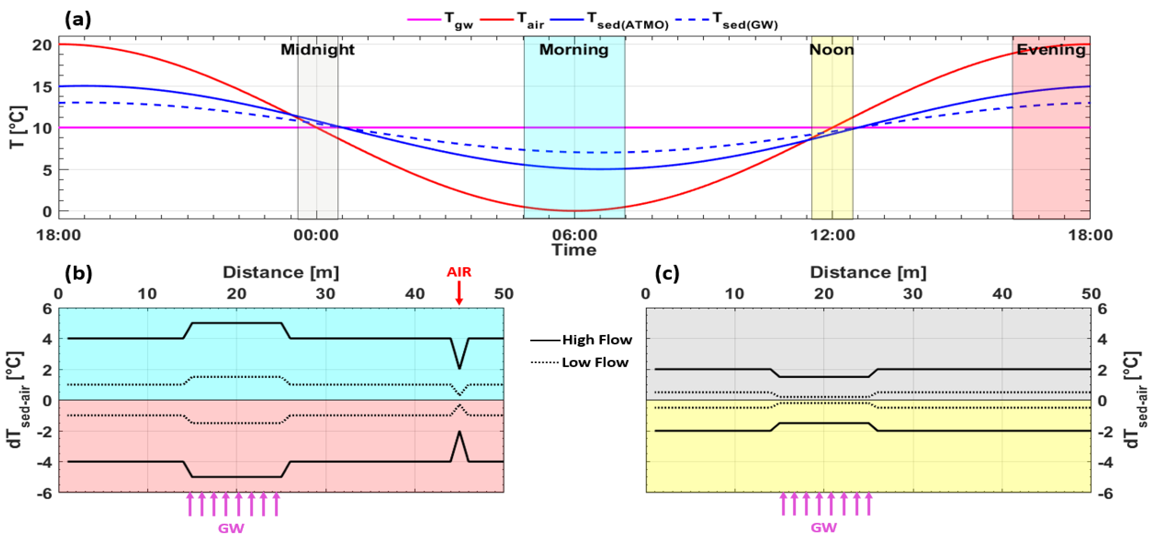
2.4. Data Post-Processing: Framework for Spatiotemporal Mapping of Groundwater Inflows

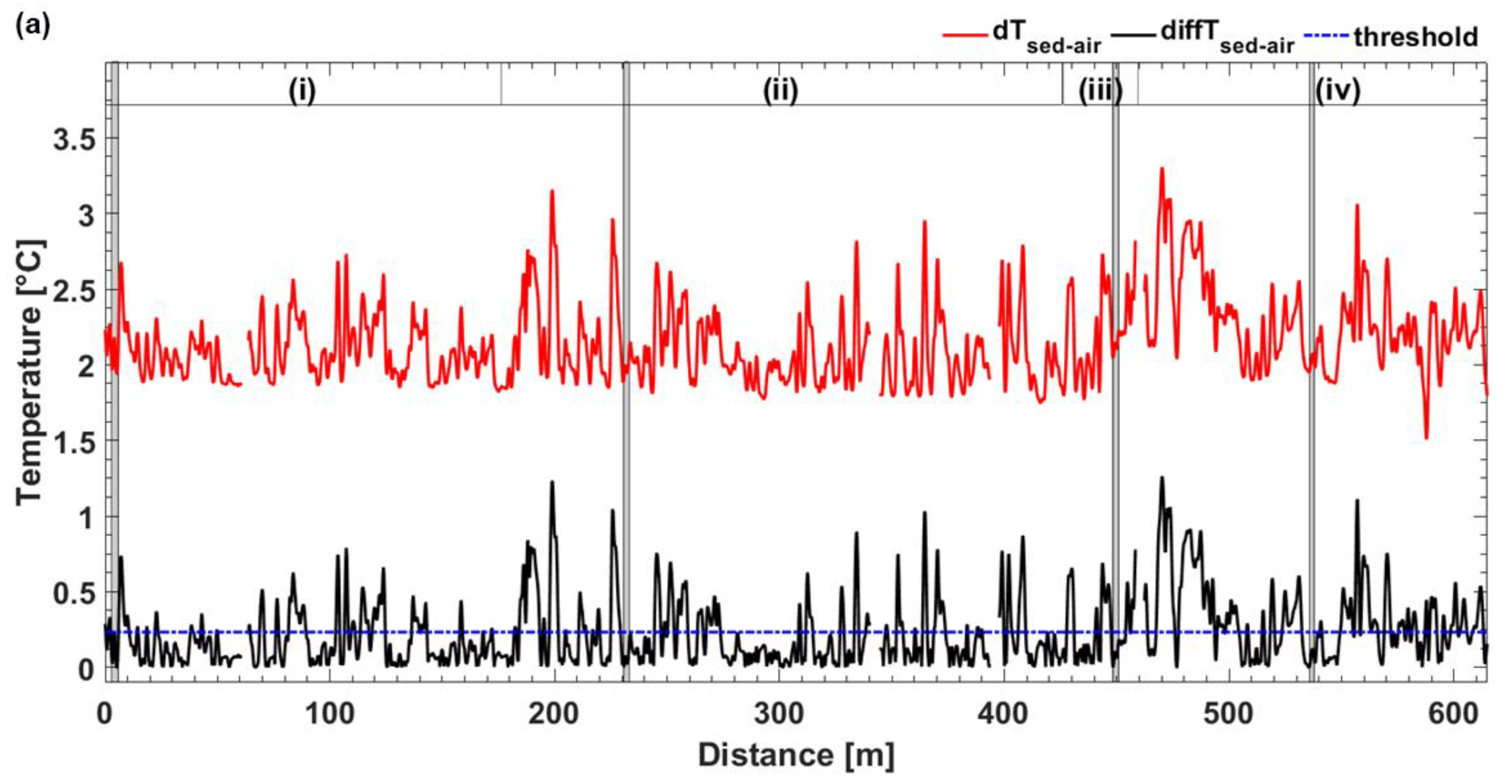
The framework depends upon a series of three hypotheses.

The first, which is widely accepted, is that streamwater temperature (T_sw) varies in a range between T_air and groundwater temperature (T_gw) (Figure 3a). Evans et al. [61] stated that more than 80% of total thermal exchanges in streams occur at the air–water interface. By contrast, Caissie [60] demonstrated that groundwater, with approximately 15% of total thermal exchanges, tends to buffer the atmosphere’s influence on stream temperature. Thus, T_sw should be closer to T_air than T_gw, regardless of the season or the hour, but it will be closer to T_gw when groundwater inflows are strong.

The second hypothesis, which is the first one in our framework, is to consider T_sed (obtained with FO-DTS) as similar to T_sw in order to have continuous information along the stream. Therefore, combining the two hypotheses, the first step to detect groundwater inflows is to calculate the thermal difference between T_sed and T_air at each point (i) and each timestep (t):

$${\mathrm{dT}}_{\mathrm{sed}-\mathrm{air}\left(t,i\right)}={\mathrm{T}}_{\mathrm{sed}\left(t,i\right)}-{\mathrm{T}}_{\mathrm{air}\left(t\right)}.$$

(1)

This simple thermal contrast summarizes a conceptual presentation of temperature effects of the two main compartments (i.e., atmosphere (T_air) and groundwater (T_gw)) on those of shallow sediment (T_sed) (Figure 3a).

The conceptual diagram of the theory underlying the study’s framework is presented Figure 3. Based on data analysis, it is assumed that the sediment temperature of a stream point influenced by groundwater varies less diurnally and is closer to T_gw than that of a point influenced only by the atmosphere. T_sed lags slightly behind T_air because T_sed requires time to react to T_air. Depending on latitude, climate, geomorphology, and season, T_air differs most from T_gw in the morning (coldest) and evening (warmest) (Figure 3b), and differs least from T_gw around midnight and midday (transitional periods) (Figure 3c). When T_air and T_gw differ the most (morning and evening), the amplitude of dT_sed-air always increases under groundwater influence (Figure 3b). When T_air and T_gw differ the least (midnight and midday), the relation between dT_sed-air and groundwater inflow is inverted: the amplitude of dT_sed-air always decreases under groundwater influence because T_sed requires time to react to T_air (Figure 3c). Regardless of the difference between T_air and T_gw, periods of high flow have much higher amplitude than those of low flow because the additional water volume of high water has more thermal inertia, which requires much more energy to increase in temperature (Figure 3b,c). Consequently, the atmosphere has less influence on stream temperature.

The third hypothesis, formulated from the previous concept (Figure 3), consists of normalizing thermal contrast using a reference point assumed to lie outside of groundwater influence. Additionally, since the information sought (groundwater influence) is related to the thermal contrast’s amplitude and not its sign, the absolute value is calculated for clarity:

$${\mathrm{diffT}}_{\mathrm{sed}-\mathrm{air}\left(t,i\right)}=\left|{\mathrm{dT}}_{\mathrm{sed}-\mathrm{air}\left(t,i\right)}-\min \left({\mathrm{dT}}_{\mathrm{sed}-\mathrm{air}\left(t,\mathrm{ref}\right)}\right)\right|$$

(2)

where dT_{sed-air(t,ref)} is the difference between T_air and T_sed at timestep t in a reference segment ref with no groundwater inflow. In Equation (2), the minimum value of dT_{sed-air(t,ref)} (i.e., that closest to T_air) in the reference segment is used to normalize data.

Like sunlight exposure, water stage and overall flow rate (no tributaries) can greatly change the influence of T_air [59,60,77,78]. These factors also vary along the stream, and special care should be taken for streams with clear and/or shallow water, such as those in our study area, since direct sunlight can influence FO-DTS measurements [79]. Ultimately, there were three requirements to for successful use of this method: (1) identify subreaches with similar geomorphology, (2) identify reference points for each reach, and (3) determine a threshold beyond which a diffT_sed-air can be attributed to groundwater inflow. To this end, thermal contrast was normalized using a reference segment (Equation (2)) for each stream subreach.

The subreaches were determined empirically based on the overall sunlight exposure (shading and orientation) and whether a tributary was present or not. Thus, four geomorphological subreaches were defined, similar to those previously described (Figure 1 and Figure 2):

(i)

The wetland, with a relatively straight channel, shallow flow and almost no high riparian vegetation;

(ii)

The woods and upstream part of the meadow, with more pronounced meandering, alternating riffles and pools, and high trees or banks;

(iii)

The downstream part of the meadow (including the bridge and the section after it), shaded with low trees and with a large streambed;

(iv)

The swamp beyond the confluence with the Vilqué, always shaded with taller trees, larger meanders, and deeper flow, with alternating riffles and pools.

The reference points were determined based on diffT_sed-air dynamics. According to our hypotheses, points influenced only by the atmosphere should have the lowest values, except for points outside of the stream or when dT_sed-air ≈ 0 °C. First, for each subreach, short cable segments with low dT_sed-air—suggesting a strong atmospheric influence—were selected. These reference segments were preferentially chosen upstream of each subreach. Then, each potential reference segment was visually analyzed over time to exclude points accidentally exposed to the atmosphere. Finally, for each subreach and each timestep t, the minimum value of dT_sed-air was selected and used to normalize data (Equation (2)).

Once normalized to their respective reference, the data from each subreach became more easily comparable. Small fluctuations in diffT_sed-air remained, but they could be explained by a buffering effect due to different water stages (riffle, pool) or different depths of burial in the sediment. To automatically select locations most likely due to groundwater inflows and not only the buffering effect, a simple threshold was applied. The mean value of diffT_sed-air along the entire monitored reach was calculated for each timestep: any points with values over it were considered potential anomalies due to groundwater inflows, while values below it were considered to be influenced by the atmosphere.

3. Results and Discussion

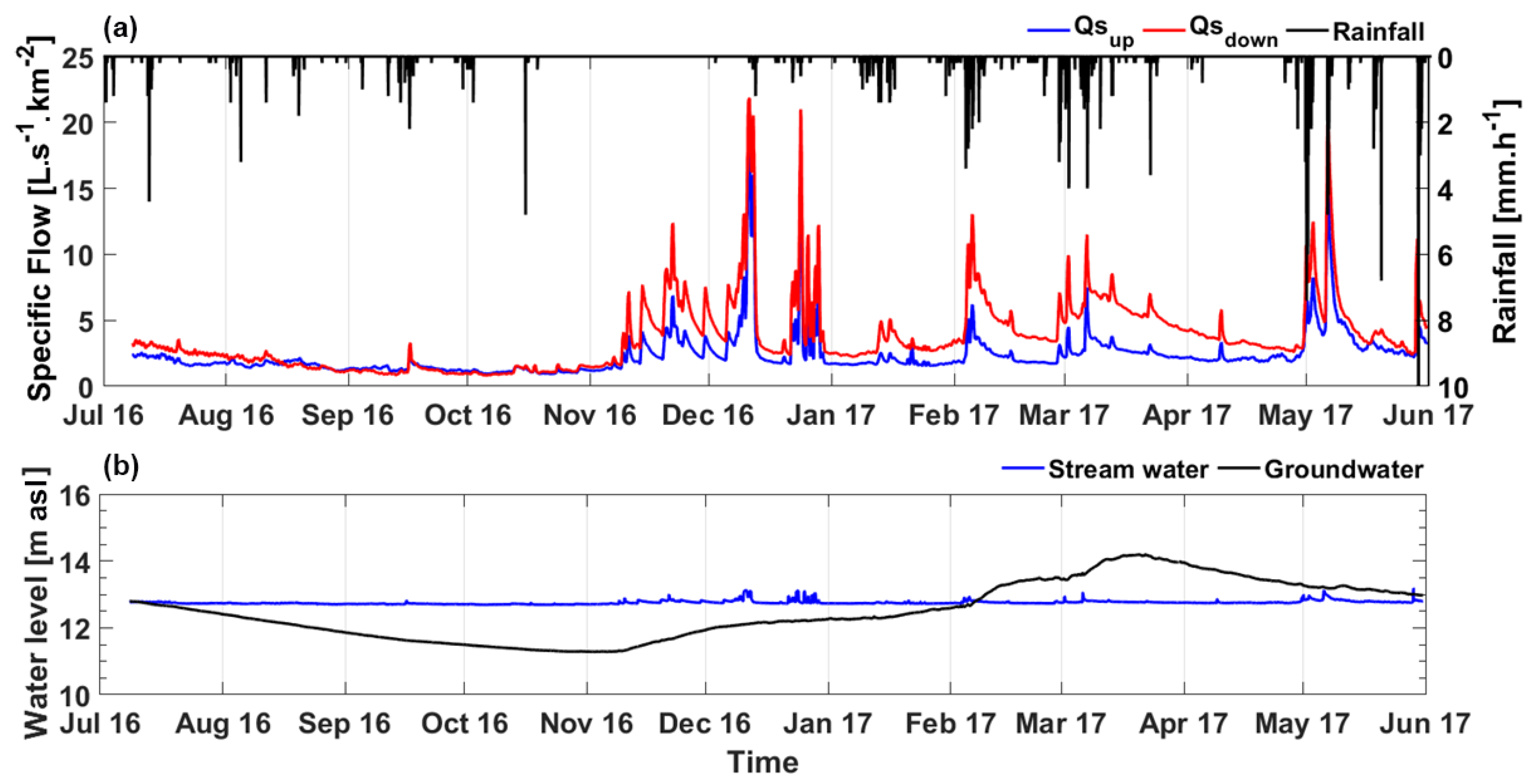
3.1. Flow Variability and Hydrological Behavior

From July to mid-November 2016, the stream had low specific discharge (1.2–2.8 L s⁻¹ km⁻²), both upstream of the site (Q_sup) and more downstream, in the site’s meadow (Qs_down) (Figure 4a). Despite a few storm events from 16 July to 16 November, almost no floods were recorded in the stream, and both upstream and downstream discharges remained similar. A few episodes in which Qs_down decreased to Q_sup were observed in August and September 2016, indicating possible losses along the reach. However, the reality of losses is difficult to assess because of uncertainty in the gauging measurements. This period from July to mid-November 2016 was qualified as low flow.

By contrast, from late November 2016 to June 2017, the site had much larger specific discharge (up to 20 L s⁻¹ km⁻² in December), which would have been due to longer rainfall periods (Figure 4a). Unfortunately, no rainfall was recorded in autumn due to a malfunction in the weather station. During this period, Qs_down began to exceed Q_sup during storm events and even during periods with no rain, after the recession limb (Figure 4a). For instance, the difference increased from ca. 0.8 to 1.6 L s⁻¹ km⁻² during January, to 3.0 L s⁻¹ km⁻² in early March, although successive storm events increased uncertainty in baseflow estimates. Afterwards, the difference decreased until late May, when the locations had similar specific discharge (2.6 L s⁻¹ km⁻²). These observations of Qs_down higher than Q_sup when no runoff was recorded tended to indicate a gaining reach from at least December to March. Thus, the period from late November 2016 to May 2017, with successive floods and an overall increase in baseflow, was qualified as high flow. Flow variability provides a comprehensive means of assessing hydrological behavior [80]. Groundwater discharge seemed to be synchronized with the low-flow period (July to mid-November 2016), with the groundwater level in the upstream wetland subreach decreasing from ca. 13.0 to 11.3 m asl by mid-November (Figure 4b). During this period, the streamwater level remained at ca. 12.7 m asl. Recharge also began when high flow began in late November; however, groundwater remained lower than the stream (negative hydraulic gradient) until February (12.8 m asl). This behavior appeared unusual for the site, where the hydraulic gradient usually becomes positive as early as December. This extended recharge period was attributed to an exceptionally dry year for the area and perhaps the fact that the streambed had been raised (Figure 2). Ultimately, this upstream subreach had positive hydraulic gradient only from February to May 2017.

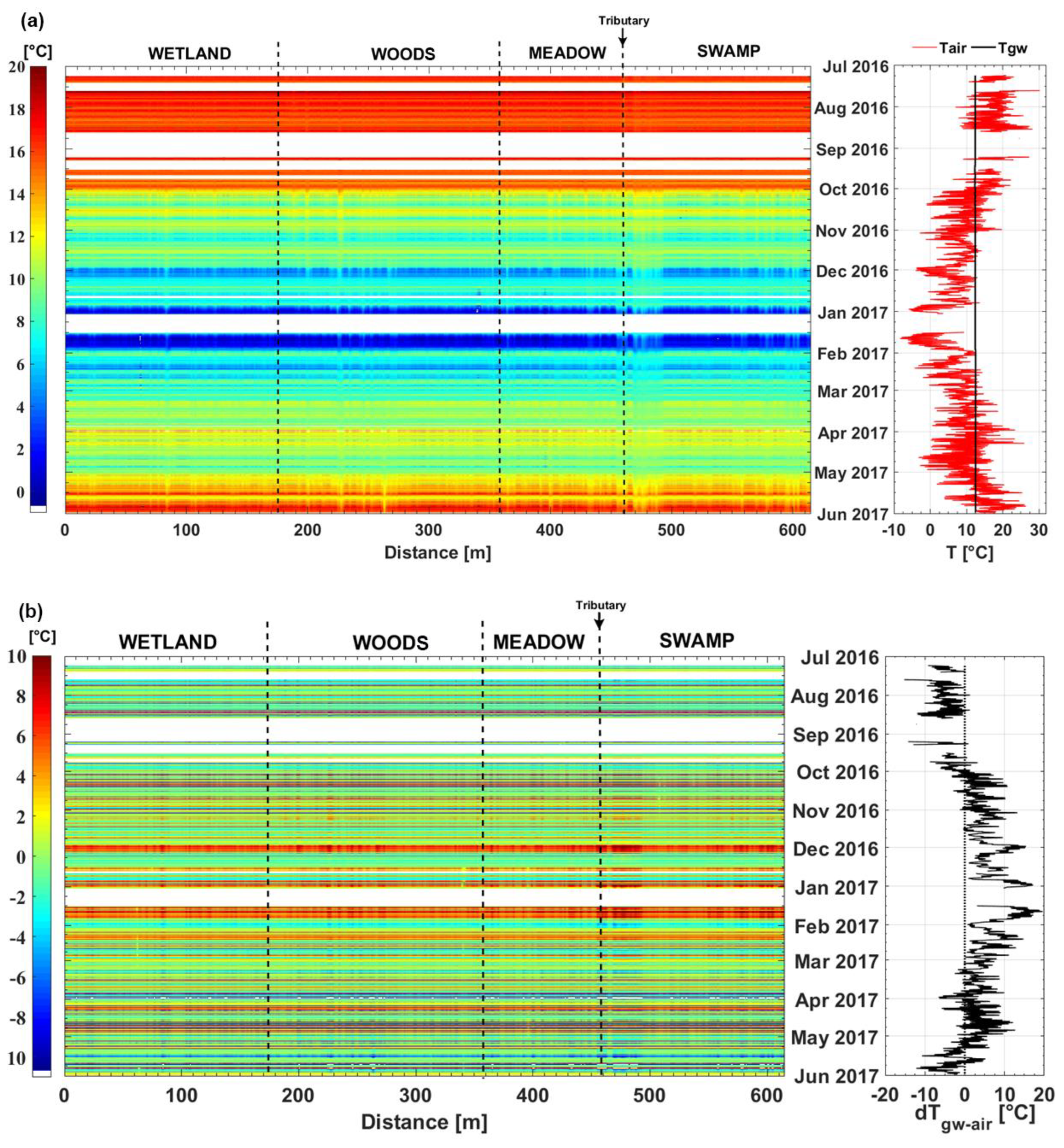
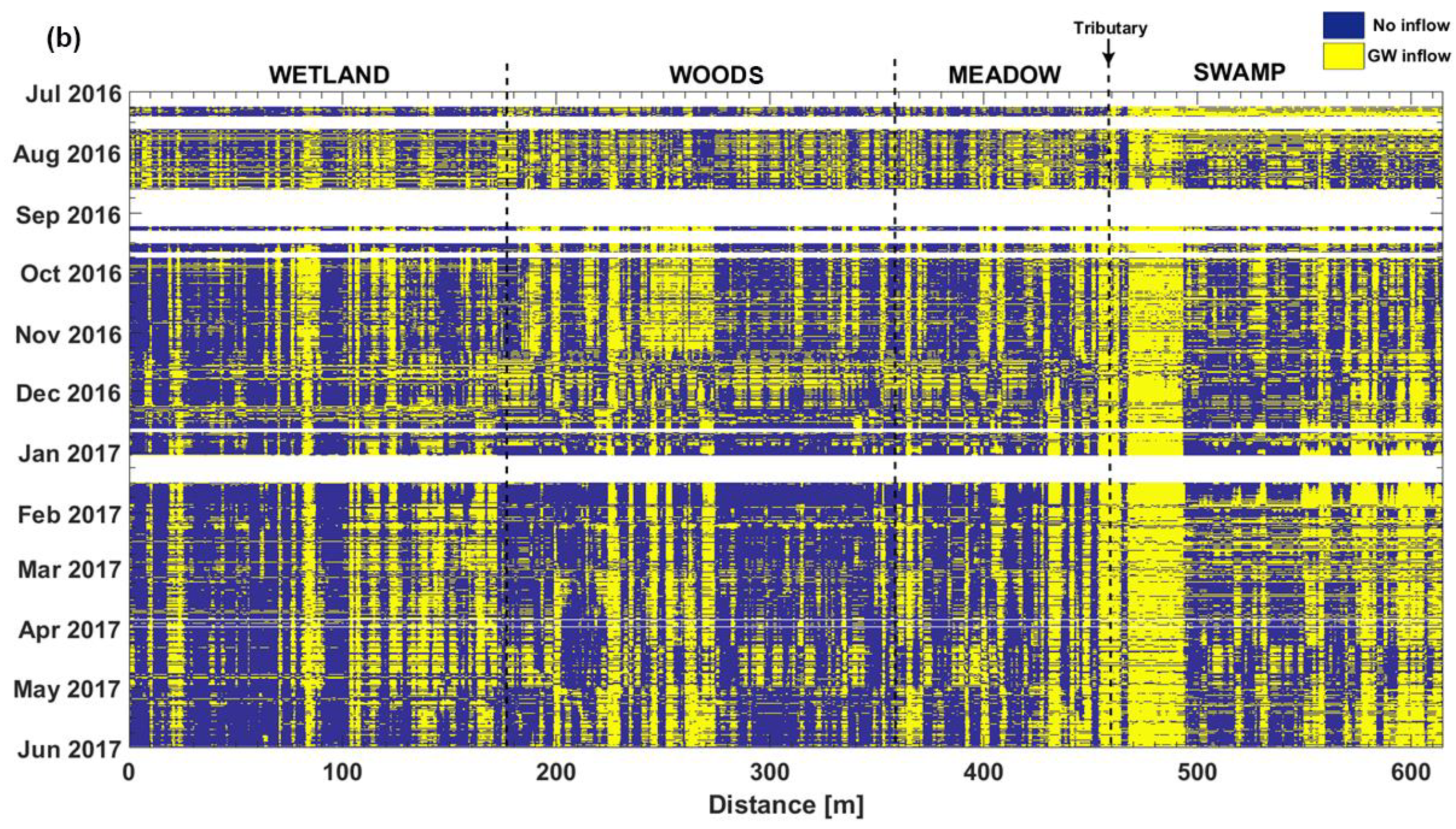
3.2. Groundwater Inflow Mapping over Time and Space

Discharge and topography provided good insight into the hydrological processes involved. During low flow, the stream lost water, most likely in its upstream wetland subreach. During high flow and between storm events (e.g., early January 2017), discharge increased from upstream to downstream gauging stations, indicating groundwater inflows.

During the low-flow period (July to October 2016), T_sed was relatively high because T_air exceeded T_gw (Figure 5a). During the high-flow period (late November 2016 to May 2017), T_gw minus T_air (dT_gw-air) became increasingly positive, indicating the colder seasons of autumn and winter. T_sed followed this trend, decreasing to a minimum in late January before increasing again in spring. Within this overall synchronicity between T_air and Tsed, certain points in the stream reacted differently over time. For instance, several points in the sediment ca. 230 m (woods) and 475 m (swamp) from the beginning of the cable appeared cooler during warm periods and warmer during cold periods than the rest of the stream (Figure 5a).

Examination of dT_sed-air showed not only these points of thermal anomaly but also periods during which T_sed of the entire stream deviated from T_air (Figure 5b). In addition, T_sed-air of some of the points of thermal anomaly remained close to zero throughout the year (62, 350, 395, and 460 m), indicating artifacts due to non-submerged cable segments. Temporally, T_sed-air varied more when T_air was close to T_gw (e.g., September to November 2016, March to May 2017), shifting between positive and negative values. Notably, during the transition from low flow to high flow (December 2016 to February 2017), dT_sed-air and dT_gw-air had high values at the same time. This high variability of dT_sed-air illustrated the combined effect of a rapidly changing T_air and the lag time of T_sed. Because this behavior made interpretation more difficult, data were normalized to distinguish groundwater inflows from atmosphere-induced artifacts.

After normalizing each subreach thermal anomaly, we observed large heterogeneities over time and space along the Petit Hermitage. Subreaches had many points with no groundwater inflows detected: the entire upstream wetland (0–180 m), the end of the woods (290–380 m), the entire meadow (380–450 m), and the middle of the swamp (500–540 m) (Figure 6b). The absence of thermal anomalies in the wetland subreach was most likely due to the perched streambed of the upstream zone, which likely made it lose water. The woods and swamp subreaches had several riffles (the latter from 500 to 550 m), and their higher elevations may have prevented groundwater inflows. By contrast, the meadow was more heterogeneous: although generally free of inflows during low flow (July to December), clear inflows appeared from January to June 2017. Thus, the swamp clearly experienced a seasonal effect in which groundwater flow paths were mobilized during high flow. Segments of the meadow always free of groundwater inflows (370–400 m) could also have been so because of several riffles.

The groundwater inflows themselves displayed different patterns throughout the year, such as intermittent and diffuse patterns in the meadow but constant patterns in the swamp. Constant inflows in the wetland (e.g., at 25 and 85 m) were apparently unrelated to streambed topography but could have been due to deep groundwater flow paths from the opposite, non-instrumented, side of the stream. Indeed, in the wetland, the stream’s right side has a much steeper bank and is much closer to the hill; thus, the groundwater level in the right hillslope may have been higher than that measured in the left hillslope (Figure 4b). The potential of a distant groundwater flow path is also supported by the position of the cable in the thalweg, which has a greater probability of intercepting this kind of deep circulation [69,81]. Constant inflows were also detected in a segment of the wetland and woods subreaches (100–280 m), but they could not be related to any parameters besides proximity to the hillslope and the natural streambed (100–200 m) or the relatively low elevation (210–260 m) (Figure 6b). In addition, a seasonal effect starting in November 2016 may have increased inflows from 150–250 m. Finally, the segment of the swamp subreach after the confluence (460–614 m) was dominated mostly by inflows throughout the year. The especially clear inflow signal from 460 to 500 m may have been related to it occurring in the deepest pool recorded at the site.

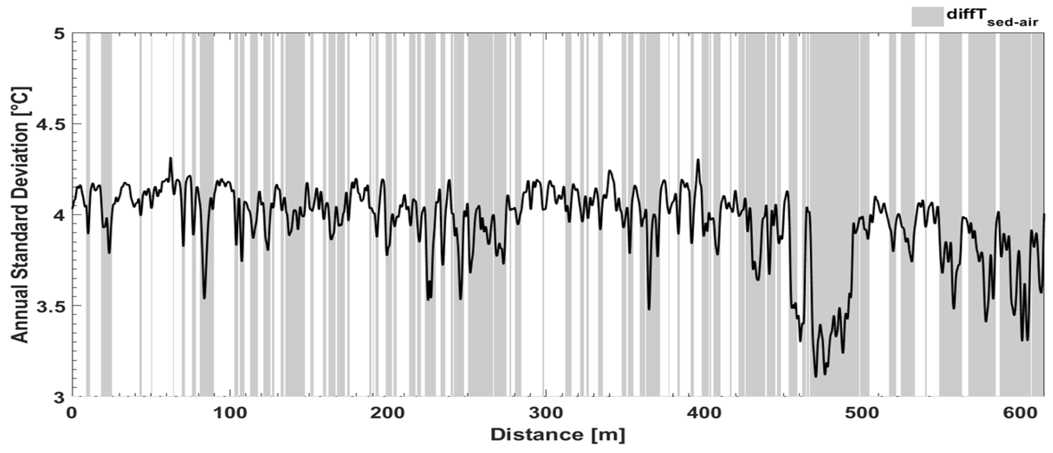
3.3. Comparing the SD Method and Framework Based on DTS

The thermal anomalies mapped using our framework were usually considered to be likely groundwater inflows. Comparing our results to the annual SD of T_sed shows that most low SDs were associated with diffuse and intermittent groundwater inflows detected more than half of the year, and vice versa (Figure 7). However, certain inflows detected more than half of the year (Figure 7) had a smaller spatial extent than those detected during shorter periods (e.g., 310–460 m during high flow) (Figure 6b). Other arguments support the groundwater inflow hypothesis. For example, some anomalies appeared at beginning of the high-flow period, especially in the meadow (310–460 m), as indicated by the net gain in discharge identified by differential gauging of Q_sup and Q_sdown. Moreover, most anomalies were located in pools, where intersection with groundwater was the most likely. Many studies have demonstrated that a hydraulic head gradient from upstream to downstream of a pool–riffle sequence is the cause of upwelling at the riffle tail [82,83,84]. In a study focused on water exchange between a stream and adjacent aquifer, Harvey et al. [85] showed that flow from the sediment to the stream occurred at transitions from steps to pools and vice versa. In our study, the generally continuous and turbulent stream flow throughout the year was considered sufficient to prevent thermal stratification, which also could have explained such differences in pools [86,87,88]. In addition, the downstream segment beyond 460 m lies in the swamp. Consequently, its banks and the surroundings were flooded or wet most of the year, indicating a likely positive hydraulic gradient from groundwater to the stream, which may explain the dense anomalies detected there (except for the shallowest sections).

Despite this indirect evidence, the nature of these thermal anomalies can be discussed further. For instance, Norman et al. [89] investigated, through flume experiments, the effects of bed topography on hyporheic flow. They identified that some anomalies could be caused by hyporheic flow recirculation instead of groundwater inflows. A cable buried deeper in the sediment may also experience greater lag time after the atmospheric signal. When our cable was removed, however, it had not been buried much deeper, except perhaps in the deepest pools, where estimating depth was difficult. In some locations (100–350 m), cable segments were uncovered by movement of the streambed [62] or even tangled up with branches and leaves. Nonetheless, the points directly in the streamwater, with low diffT_sed-air, did not behave so differently that they modified the detection threshold. Only segments of cable found non-submerged differed significantly (diffT_sed-air ≈ 0) and were removed from the dataset. Even though the method still needs improvement, this study underscored the need to consider patterns and change in groundwater inflows over a long temporal scale completed by the Part II of this study focused on groundwater inflow quantification by coupling FO-DTS and vertical velocities inferred from thermal lances profiles in the hyporheic zone [90].

4. Conclusions

The concepts and relations developed in this study provide a useful and simple methodology to analyze a large database of stream temperature at high spatial and temporal resolution over a one-year period using FO-DTS. We used a simple approach based on thermal contrast normalized by a reference point assumed to lie outside of groundwater influence. The framework depends on a set of hypotheses for characterizing spatial heterogeneity and temporal intermittency and mapping groundwater inflow. Results highlighted the main temporal scale needed to identify effects from groundwater or the atmosphere. Diurnal temperature variation, as well as seasonal variability (high- and low-water periods), provided conceptual interpretation of thermal anomalies for determining patterns of groundwater–surface water exchange. Streambed topography was also important: riffle-and-pool sequences and perched reaches had many fewer inflows than pools. In addition, the spatial extent of groundwater inflows increased at some locations during the high-flow period. During high flow, the usual SD approach located the same inflows but underestimated their extent because the SD was integrated over the entire year. The inflow mapping method showed a clear distribution of groundwater inflows consistent with previous studies of the same stream. However, the results of thermal anomaly mapping could not distinguish groundwater inflows from hyporheic recirculation or overbuffering from sediment. Additional onsite piezometric measurements, vertical flow measurements in the hyporheic zone, and/or the use of isotopes and chemical tracers could help to determine the processes involved and identify sources and sinks. Also, mapping temporal intermittency can help improve the analysis and identification of biogeochemical and hydrological processes, especially in heterogeneous streams with geomorphological contrast or heavy human modification. This method may prove useful in domains such as hydrological modeling and environmental management, which require high spatial resolution and high-frequency data.

References

1. Cox, M.H.; Su, G.W.; Constantz, J. Heat, chloride, and specific conductance as ground water tracers near streams. Ground Water 2007, 45, 187–195. [Google Scholar] [CrossRef]
2. Dybkjaer, J.B.; Baattrup-Pedersen, A.; Kronvang, B.; Thodsen, H. Diversity and Distribution of Riparian Plant Communities in Relation to Stream Size and Eutrophication. J. Environ. Qual. 2012, 41, 348–354. [Google Scholar] [CrossRef]
3. Ebersole, J.L.; Liss, W.J.; Frissell, C.A. Cold water patches in warm streams: Physicochemical characteristics and the influence of shading. J. Am. Water Resour. Assoc. 2003, 39, 355–368. [Google Scholar] [CrossRef]
4. Fernald, A.G.; Landers, D.H.; Wigington, P.J. Water quality changes in hyporheic flow paths between a large gravel bed river and off-channel alcoves in Oregon, USA. River Res. Appl. 2006, 22, 1111–1124. [Google Scholar] [CrossRef]
5. Vidon, P.; Allan, C.; Burns, D.; Duval, T.P.; Gurwick, N.; Inamdar, S.; Lowrance, R.; Okay, J.; Scott, D.; Sebestyen, S. Hot Spots and Hot Moments in Riparian Zones: Potential for Improved Water Quality Management1. J. Am. Water Resour. Assoc. 2010, 46, 278–298. [Google Scholar] [CrossRef]
6. Bucak, T.; Trolle, D.; Andersen, H.E.; Thodsen, H.; Erdogan, S.; Levi, E.E.; Filiz, N.; Jeppesen, E.; Beklioglu, M. Future water availability in the largest freshwater Mediterranean lake is at great risk as evidenced from simulations with the SWAT model. Sci. Total Environ. 2017, 581, 413–425. [Google Scholar] [CrossRef]
7. Freeze, R.A. Role of subsurface flow in generating surface runoff: 1. Base flow contributions to channel flow. Water Resour. Res. 1972, 8, 609–623. [Google Scholar] [CrossRef]
8. Hester, E.T.; Gooseff, M.N. Moving Beyond the Banks: Hyporheic Restoration Is Fundamental to Restoring Ecological Services and Functions of Streams. Environ. Sci. Technol. 2010, 44, 1521–1525. [Google Scholar] [CrossRef]
9. Kunkle, G.R. Computation of ground-water discharge to streams during floods, or to individual reaches during base flow, by use of specific conductance. In US Geological Survey Professional Paper; U.S. Geological Survey: Reston, VA, USA, 1965; pp. 207–210. [Google Scholar]
10. Nathan, R.; McMahon, T. Evaluation of automated techniques for base flow and recession analyses. Water Resour. Res. 1990, 26, 1465–1473. [Google Scholar] [CrossRef]
11. Wittenberg, H. Baseflow recession and recharge as nonlinear storage processes. Hydrol. Process. 1999, 13, 715–726. [Google Scholar] [CrossRef]
12. Alexander, M.D.; Caissie, D. Variability and comparison of hyporheic water temperatures and seepage fluxes in a small Atlantic salmon stream. Ground Water 2003, 41, 72–82. [Google Scholar] [CrossRef] [PubMed]
13. Dugdale, S.J.; Bergeron, N.E.; St-Hilaire, A. Temporal variability of thermal refuges and water temperature patterns in an Atlantic salmon river. Remote Sens. Environ. 2013, 136, 358–373. [Google Scholar] [CrossRef]
14. Dugdale, S.J.; Bergeron, N.E.; St-Hilaire, A. Spatial distribution of thermal refuges analysed in relation to riverscape hydromorphology using airborne thermal infrared imagery. Remote Sens. Environ. 2015, 160, 43–55. [Google Scholar] [CrossRef]
15. Ebersole, J.L.; Liss, W.J.; Frissell, C.A. Thermal heterogeneity, stream channel morphology, and salmonid abundance in northeastern Oregon streams. Can. J. Fish. Aquat. Sci. 2003, 60, 1266–1280. [Google Scholar] [CrossRef]
16. Ficke, A.D.; Myrick, C.A.; Hansen, L.J. Potential impacts of global climate change on freshwater fisheries. Rev. Fish Biol. Fish. 2007, 17, 581–613. [Google Scholar] [CrossRef]
17. Hester, E.T.; Doyle, M.W. Human Impacts to River Temperature and Their Effects on Biological Processes: A Quantitative Synthesis. J. Am. Water Resour. Assoc. 2011, 47, 571–587. [Google Scholar] [CrossRef]
18. Hillyard, R.W.; Keeley, E.R. Temperature-Related Changes in Habitat Quality and Use by Bonneville Cutthroat Trout in Regulated and Unregulated River Segments. Trans. Am. Fish. Soc. 2012, 141, 1649–1663. [Google Scholar] [CrossRef]
19. Lane, C.R.; Flotemersch, J.E.; Blocksom, K.A.; Decelles, S. Effect of sampling method on diatom composition for use in monitoring and assessing large river condition. River Res. Appl. 2007, 23, 1126–1146. [Google Scholar] [CrossRef]
20. Lisi, P.J.; Schindler, D.E.; Bentley, K.T.; Pess, G.R. Association between geomorphic attributes of watersheds, water temperature, and salmon spawn timing in Alaskan streams. Geomorphology 2013, 185, 78–86. [Google Scholar] [CrossRef]
21. Magoulick, D.D.; Kobza, R.M. The role of refugia for fishes during drought: A review and synthesis. Freshw. Biol. 2003, 48, 1186–1198. [Google Scholar] [CrossRef]
22. Baattrup-Pedersen, A.; Jensen, K.M.B.; Thodsen, H.; Andersen, H.E.; Andersen, P.M.; Larsen, S.E.; Riis, T.; Andersen, D.K.; Audet, J.; Kronvang, B. Effects of stream flooding on the distribution and diversity of groundwater-dependent vegetation in riparian areas. Freshw. Biol. 2013, 58, 817–827. [Google Scholar] [CrossRef]
23. Bayley, P.B. The flood pulse advantage and the restoration of river-floodplain systems. Regul. Rivers Res. Manag. 1991, 6, 75–86. [Google Scholar] [CrossRef]
24. Brown, A.G.; Lespez, L.; Sear, D.A.; Macaire, J.-J.; Houben, P.; Klimek, K.; Brazier, R.E.; Van Oost, K.; Pears, B. Natural vs. anthropogenic streams in Europe: History, ecology and implications for restoration, river-rewilding and riverine ecosystem services. Earth-Sci. Rev. 2018, 180, 185–205. [Google Scholar] [CrossRef]
25. Burkholder, B.K.; Grant, G.E.; Haggerty, R.; Khangaonkar, T.; Wampler, P.J. Influence of hyporheic flow and geomorphology on temperature of a large, gravel-bed river, Clackamas River, Oregon, USA. Hydrol. Process. 2008, 22, 941–953. [Google Scholar] [CrossRef]
26. Kurth, A.M.; Weber, C.; Schirmer, M. How effective is river restoration in re-establishing groundwater-surface water interactions?—A case study. Hydrol. Earth Syst. Sci. 2015, 19, 2663–2672. [Google Scholar] [CrossRef]
27. Hester, E.T.; Doyle, M.W.; Poole, G.C. The influence of in-stream structures on summer water temperatures via induced hyporheic exchange. Limnol. Oceanogr. 2009, 54, 355–367. [Google Scholar] [CrossRef]
28. Wawrzyniak, V.; Piégay, H.; Allemand, P.; Vaudor, L.; Goma, R.; Grandjean, P. Effects of geomorphology and groundwater level on the spatio-temporal variability of riverine cold water patches assessed using thermal infrared (TIR) remote sensing. Remote Sens. Environ. 2016, 175, 337–348. [Google Scholar] [CrossRef]
29. Winter, T.C. Landscape approach to identifying environments where ground water and surface water are closely interrelated. In Proceedings of the International Symposium on Groundwater Management Proceedings (ASCE, Ed.), San Antonio, TX, USA, 14–16 August 1995; pp. 139–155. [Google Scholar]
30. Varli, D.; Yilmaz, K. A Multi-Scale Approach for Improved Characterization of Surface Water—Groundwater Interactions: Integrating Thermal Remote Sensing and in-Stream Measurements. Water 2018, 10, 854. [Google Scholar] [CrossRef]
31. Fox, A.; Laube, G.; Schmidt, C.; Fleckenstein, J.H.; Arnon, S. The effect of losing and gaining flow conditions on hyporheic exchange in heterogeneous streambeds. Water Resour. Res. 2016, 52, 7460–7477. [Google Scholar] [CrossRef]
32. Genereux, D.P.; Leahy, S.; Mitasova, H.; Kennedy, C.D.; Corbett, D.R. Spatial and temporal variability of streambed hydraulic conductivity in West Bear Creek, North Carolina, USA. J. Hydrol. 2008, 358, 332–353. [Google Scholar] [CrossRef]
33. Hess, K.M.; Wolf, S.H.; Celia, M.A. Large-scale Natural gradient tracer test in sand and gravel, Cape Cod, Massachusetts 3. Hydraulic conductivity variability and calculated macrodispersivities. Water Resour. Res. 1992, 28, 2011–2027. [Google Scholar] [CrossRef]
34. Fleckenstein, J.H.; Niswonger, R.G.; Fogg, G.E. River-aquifer interactions, geologic heterogeneity, and low-flow management. Ground Water 2006, 44, 837–852. [Google Scholar] [CrossRef] [PubMed]
35. Schilling, O.S.; Irvine, D.J.; Hendricks Franssen, H.-J.; Brunner, P. Estimating the Spatial Extent of Unsaturated Zones in Heterogeneous River-Aquifer Systems. Water Resour. Res. 2017, 53, 10583–10602. [Google Scholar] [CrossRef] [Green Version]
36. Wroblicky, G.J.; Campana, M.E.; Valett, H.M.; Dahm, C.N. Seasonal variation in surface-subsurface water exchange and lateral hyporheic area of two stream-aquifer systems. Water Resour. Res. 1998, 34, 317–328. [Google Scholar] [CrossRef]
37. Mojarrad, B.B.; Riml, J.; Wörman, A.; Laudon, H. Fragmentation of the Hyporheic Zone Due to Regional Groundwater Circulation. Water Resour. Res. 2019, 55, 1242–1262. [Google Scholar] [CrossRef]
38. Kalbus, E.; Reinstorf, F.; Schirmer, M. Measuring methods for groundwater—surface water interactions: A review. Hydrol. Earth Syst. Sci. 2006, 10, 873–887. [Google Scholar] [CrossRef] [Green Version]
39. Griebler, C.; Lueders, T. Microbial biodiversity in groundwater ecosystems. Freshw. Biol. 2009, 54, 649–677. [Google Scholar] [CrossRef]
40. Iribar, A.; Sánchez-Pérez, J.M.; Lyautey, E.; Garabétian, F. Differentiated free-living and sediment-attached bacterial community structure inside and outside denitrification hotspots in the river–groundwater interface. Hydrobiologia 2008, 598, 109–121. [Google Scholar] [CrossRef]
41. Malard, F.; Hervant, F. Oxygen supply and the adaptations of animals in groundwater. Freshw. Biol. 1999, 41, 1–30. [Google Scholar] [CrossRef]
42. Frei, S.; Gilfedder, B.S. FINIFLUX: An implicit finite element model for quantification of groundwater fluxes and hyporheic exchange in streams and rivers using radon. Water Resour. Res. 2015, 51, 6776–6786. [Google Scholar] [CrossRef] [Green Version]
43. Frei, S.; Durejka, S.; Le Lay, H.; Thomas, Z.; Gilfedder, B.S. Hyporheic nitrate removal at the reach scale: Exposure times vs. residence times. Water Resour. Res. 2019, in press. [Google Scholar] [CrossRef] [Green Version]
44. Genereux, D.P.; Hemond, H.F.; Mulholland, P.J. Use of radon-222 and calcium as tracers in a three-end-member mixing model for streamflow generation on the West Fork of Walker Branch Watershed. J. Hydrol. 1993, 142, 167–211. [Google Scholar] [CrossRef]
45. Kaandorp, V.P.; Doornenbal, P.J.; Kooi, H.; Peter Broers, H.; de Louw, P.G.B. Temperature buffering by groundwater in ecologically valuable lowland streams under current and future climate conditions. J. Hydrol. 2019, 3, 1–16. [Google Scholar] [CrossRef]
46. Mullinger, N.J.; Pates, J.M.; Binley, A.M.; Crook, N.P. Controls on the spatial and temporal variability of Rn-222 in riparian groundwater in a lowland Chalk catchment. J. Hydrol. 2009, 376, 58–69. [Google Scholar] [CrossRef] [Green Version]
47. Anderson, M.P. Heat as a ground water tracer. Ground Water 2005, 43, 951–968. [Google Scholar] [CrossRef]
48. Avery, E.; Bibby, R.; Visser, A.; Esser, B.; Moran, J. Quantification of Groundwater Discharge in a Subalpine Stream Using Radon-222. Water 2018, 10, 100. [Google Scholar] [CrossRef] [Green Version]
49. Constantz, J. Interaction between stream temperature, streamflow, and groundwater exchanges in Alpine streams. Water Resour. Res. 1998, 34, 1609–1615. [Google Scholar] [CrossRef]
50. Constantz, J. Heat as a tracer to determine streambed water exchanges. Water Resour. Res. 2008, 44, 1–20. [Google Scholar] [CrossRef]
51. Lee, J.-Y.; Lim, H.; Yoon, H.; Park, Y. Stream Water and Groundwater Interaction Revealed by Temperature Monitoring in Agricultural Areas. Water 2013, 5, 1677–1698. [Google Scholar] [CrossRef]
52. Schmidt, C.; Bayer-Raich, M.; Schirmer, M. Characterization of spatial heterogeneity of groundwater-stream water interactions using multiple depth streambed temperature measurements at the reach scale. Hydrogeol. Earth Syst. Sci. 2006, 10, 849–859. [Google Scholar] [CrossRef] [Green Version]
53. Harvey, M.C.; Hare, D.K.; Hackman, A.; Davenport, G.; Haynes, A.B.; Helton, A.; Lane, J.W.; Briggs, M.A. Evaluation of Stream and Wetland Restoration Using UAS-Based Thermal Infrared Mapping. Water 2019, 11, 1568. [Google Scholar] [CrossRef] [Green Version]
54. Lalot, E.; Curie, F.; Wawrzyniak, V.; Baratelli, F.; Schomburgk, S.; Flipo, N.; Piegay, H.; Moatar, F. Quantification of the contribution of the Beauce groundwater aquifer to the discharge of the Loire River using thermal infrared satellite imaging. Hydrol. Earth Syst. Sci. 2015, 19, 4479–4492. [Google Scholar] [CrossRef] [Green Version]
55. Wawrzyniak, V.; Piegay, H.; Poirel, A. Longitudinal and temporal thermal patterns of the French Rhne River using Landsat ETM plus thermal infrared images. Aquat. Sci. 2012, 74, 405–414. [Google Scholar] [CrossRef]
56. Hare, D.K.; Briggs, M.A.; Rosenberry, D.O.; Boutt, D.F.; Lane, J.W. A comparison of thermal infrared to fiber-optic distributed temperature sensing for evaluation of groundwater discharge to surface water. J. Hydrol. 2015, 530, 153–166. [Google Scholar] [CrossRef] [Green Version]
57. Hausner, M.B.; Suarez, F.; Glander, K.E.; van de Giesen, N.; Selker, J.S.; Tyler, S.W. Calibrating Single-Ended Fiber-Optic Raman Spectra Distributed Temperature Sensing Data. Sensors 2011, 11, 10859–10879. [Google Scholar] [CrossRef]
58. Tyler, S.W.; Selker, J.S.; Hausner, M.B.; Hatch, C.E.; Torgersen, T.; Thodal, C.E.; Schladow, S.G. Environmental temperature sensing using Raman spectra DTS fiber-optic methods. Water Resour. Res. 2009, 45, 11. [Google Scholar] [CrossRef] [Green Version]
59. Benyahya, L.; Caissie, D.; Satish, M.G.; El-Jabi, N. Long-wave radiation and heat flux estimates within a small tributary in Catamaran Brook (New Brunswick, Canada). Hydrol. Process. 2012, 26, 475–484. [Google Scholar] [CrossRef]
60. Caissie, D. The thermal regime of rivers: A review. Freshw. Biol. 2006, 51, 1389–1406. [Google Scholar] [CrossRef]
61. Evans, E.C.; McGregor, G.R.; Petts, G.E. River energy budgets with special reference to river bed processes. Hydrol. Process. 1998, 12, 575–595. [Google Scholar] [CrossRef]
62. Sebok, E.; Duque, C.; Engesgaard, P.; Boegh, E. Application of Distributed Temperature Sensing for coupled mapping of sedimentation processes and spatio-temporal variability of groundwater discharge in soft-bedded streams. Hydrol. Process. 2015, 29, 3408–3422. [Google Scholar] [CrossRef]
63. Collier, M.W. Demonstration of Fiber Optic Distributed Temperature Sensing to Differentiate Cold Water Refuge between Ground Water Inflows and Hyporheic Exchange. Master’ Thesis, Oregon State University, Corvallis, OR, USA, 2008. [Google Scholar]
64. Strahler, A.N. Quantitative analysis of watershed geomorphology. EosTrans. Am. Geophys. Union 1957, 38, 913–920. [Google Scholar] [CrossRef] [Green Version]
65. Jaunat, J.; Huneau, F.; Dupuy, A.; Celle-Jeanton, H.; Vergnaud-Ayraud, V.; Aquilina, L.; Labasque, T.; Le Coustumer, P. Hydrochemical data and groundwater dating to infer differential flowpaths through weathered profiles of a fractured aquifer. Appl. Geochem. 2012, 27, 2053–2067. [Google Scholar] [CrossRef]
66. Lachassagne, P.; Wyns, R.; Dewandel, B. The fracture permeability of Hard Rock Aquifers is due neither to tectonics, nor to unloading, but to weathering processes. Terra Nova 2011, 23, 145–161. [Google Scholar] [CrossRef]
67. Thomas, Z.; Rousseau-Gueutin, P.; Kolbe, T.; Abbott, B.W.; Marçais, J.; Peiffer, S.; Frei, S.; Bishop, K.; Pichelin, P.; Pinay, G.; et al. Constitution of a catchment virtual observatory for sharing flow and transport models outputs. J. Hydrol. 2016, 543, 59–66. [Google Scholar] [CrossRef] [Green Version]
68. Thomas, Z.; Rousseau-Gueutin, P.; Abbott, B.W.; Kolbe, T.; Le Lay, H.; Marçais, J.; Rouault, F.; Petton, C.; Pichelin, P.; Le Hennaff, G.; et al. Long-term ecological observatories needed to understand ecohydrological systems in the Anthropocene: A catchment-scale case study in Brittany, France. Reg. Environ. Chang. 2019, 19, 363–377. [Google Scholar] [CrossRef]
69. Kolbe, T.; Marcais, J.; Thomas, Z.; Abbott, B.W.; de Dreuzy, J.R.; Rousseau-Gueutin, P.; Aquilina, L.; Labasque, T.; Pinay, G. Coupling 3D groundwater modeling with CFC-based age dating to classify local groundwater circulation in an unconfined crystalline aquifer. J. Hydrol. 2016, 543, 31–46. [Google Scholar] [CrossRef] [Green Version]
70. Kolbe, T.; de Dreuzy, J.-R.; Abbott, B.W.; Aquilina, L.; Babey, T.; Green, C.T.; Fleckenstein, J.H.; Labasque, T.; Laverman, A.M.; Marçais, J.; et al. Stratification of reactivity determines nitrate removal in groundwater. Proc. Natl. Acad. Sci. USA 2019, 116, 2494–2499. [Google Scholar] [CrossRef] [Green Version]
71. Tirado-Conde, J.; Engesgaard, P.; Karan, S.; Müller, S.; Duque, C. Evaluation of Temperature Profiling and Seepage Meter Methods for Quantifying Submarine Groundwater Discharge to Coastal Lagoons: Impacts of Saltwater Intrusion and the Associated Thermal Regime. Water 2019, 11, 1648. [Google Scholar] [CrossRef] [Green Version]
72. Calkins, D.; Dunne, T. A salt tracing method for measuring channel velocities in small mountain streams. J. Hydrol. 1970, 11, 379–392. [Google Scholar] [CrossRef]
73. van de Giesen, N.; Steele-Dunne, S.C.; Jansen, J.; Hoes, O.; Hausner, M.B.; Tyler, S.; Selker, J. Double-Ended Calibration of Fiber-Optic Raman Spectra Distributed Temperature Sensing Data. Sensors 2012, 12, 5471–5485. [Google Scholar] [CrossRef] [Green Version]
74. Le lay, H.; Thomas, Z.; Bour, O.; Rouault, F.; Pichelin, P.; Moatar, F. Experimental and model-based investigation of the effect of the free- surface flow regime on the detection threshold of warm water inflows. Water Resour. Res. 2019, in press. [Google Scholar]
75. Krause, S.; Blume, T.; Cassidy, N. Investigating patterns and controls of groundwater up-welling in a lowland river by combining Fibre-optic Distributed Temperature Sensing with observations of vertical hydraulic gradients. Hydrol. Earth Syst. Sci. 2012, 16, 1775–1792. [Google Scholar] [CrossRef] [Green Version]
76. Lowry, C.S.; Walker, J.F.; Hunt, R.J.; Anderson, M.P. Identifying spatial variability of groundwater discharge in a wetland stream using a distributed temperature sensor. Water Resour. Res. 2007, 43, 1–9. [Google Scholar] [CrossRef]
77. Hebert, C.; Caissie, D.; Satish, M.G.; El-Jabi, N. Study of stream temperature dynamics and corresponding heat fluxes within Miramichi River catchments (New Brunswick, Canada). Hydrol. Process. 2011, 25, 2439–2455. [Google Scholar] [CrossRef]
78. Maheu, A.; Caissie, D.; St-Hilaire, A.; El-Jabi, N. River evaporation and corresponding heat fluxes in forested catchments. Hydrol. Process. 2014, 28, 5725–5738. [Google Scholar] [CrossRef]
79. Neilson, B.T.; Hatch, C.E.; Ban, H.; Tyler, S.W. Solar radiative heating of fiber optic cables used to monitor temperatures in water. Water Resour. Res. 2010, 46, 2–17. [Google Scholar] [CrossRef] [Green Version]
80. Westerberg, I.K.; Wagener, T.; Coxon, G.; McMillan, H.K.; Castellarin, A.; Montanari, A.; Freer, J. Uncertainty in hydrological signatures for gauged and ungauged catchments. Water Resour. Res. 2016, 52, 1847–1865. [Google Scholar] [CrossRef] [Green Version]
81. Toth, J. A theoretical analysis of groundwater flow in small drainage basins. J. Geophys. Res. 1963, 68, 4795–4812. [Google Scholar] [CrossRef]
82. Crispell, J.K.; Endreny, T.A. Hyporheic exchange flow around constructed in-channel structures and implications for restoration design. Hydrol. Process. 2009, 23, 1158–1168. [Google Scholar] [CrossRef]
83. Flipo, N.; Mouhri, A.; Labarthe, B.; Biancamaria, S.; Rivière, A.; Weill, P. Continental hydrosystem modelling: The concept of nested stream–aquifer interfaces. Hydrol. Earth Syst. Sci. 2014, 18, 3121–3149. [Google Scholar] [CrossRef] [Green Version]
84. Magliozzi, C.; Grabowski, R.C.; Packman, A.I.; Krause, S. Toward a conceptual framework of hyporheic exchange across spatial scales. Hydrol. Earth Syst. Sci. 2018, 22, 6163–6185. [Google Scholar] [CrossRef] [Green Version]
85. Harvey, J.W.; Bencala, K.E. The Effect of Streambed Topography on Surface-Subsurface Water Exchange in Mountain Catchments. Water Resour. Res. 1993, 29, 89–98. [Google Scholar] [CrossRef]
86. Matthews, K.R.; Berg, N.H.; Azuma, D.L.; Lambert, T.R. Cool water formation and trout habitat use in a deep pool in the sierra-nevada, california. Trans. Am. Fish. Soc. 1994, 123, 549–564. [Google Scholar] [CrossRef]
87. Nielsen, J.L.; Lisle, T.E.; Ozaki, V. Thermally stratified pools and their use by steelhead in northern california streams. Trans. Am. Fish. Soc. 1994, 123, 613–626. [Google Scholar] [CrossRef]
88. Webb, B.W.; Walling, D.E. Complex summer water temperature behaviour below a UK regulating reservoir. Regul. Rivers-Res. Manag. 1997, 13, 463–477. [Google Scholar] [CrossRef]
89. Norman, F.A.; Cardenas, M.B. Heat transport in hyporheic zones due to bedforms: An experimental study. Water Resour. Res. 2014, 50, 3568–3582. [Google Scholar] [CrossRef]
90. Le Lay, H.; Thomas, Z.; Rouault, F.; Pichelin, P.; Moatar, F. Characterization of diffuse groundwater inflows into stream water. Part II: Quantifying groundwater inflows by coupling FO-DTS and vertical flow velocities. Water 2019, in press. [Google Scholar]
Figure 1. Location of the study site in the Zone Atelier Armorique in northeastern Brittany, France (a). The monitored stream, Petit Hermitage draining a 16 km2 subwatershed whose small tributary drains a 2.34 km2 area of Vilqué stream (b). A fiber optic cable 614 m long was placed in the main stream and connected to a distributed temperature sensing (DTS) unit in a nearby building (c). A piezometer was previously installed upstream of the site, as were gauging stations in the stream. Black lines indicate boundaries between subreaches with different geomorphologies. A weather station lies ca. 1 km to the north of the site (outside the map).
Water 11 02389 g001
Figure 2. 3D view of the study area indicating the hillslope cross section of the upstream hillslope adjacent to the wetland sub-reach and longitudinal profile of the streambed of the Petit Hermitage. Hillslope cross section shows locations and depths of piezometers, including the one (blue diamond) used for groundwater temperature measurements (Tgw) and groundwater level for high water (HW) -dashed blue line- and low water (LW) -dashed green line period-. Tsed (FO-DTS) = sediment temperature from fiber optic distributed temperature sensing, m asl = m above sea level.
Water 11 02389 g002
Figure 3. Conceptual diagram of the theory underlying the study’s framework. (a) Theoretical diurnal temperatures of the atmosphere (Tair), groundwater (Tgw), and the sediment influenced mainly by each of them (Tsed (ATMO) and Tsed (GW), respectively). (Bottom) Theoretical differences between sediment and air temperatures (dTsed-air) (Equation (1)) under high or low flow (b) in the morning and evening or (c) at midnight and midday along a given reach with groundwater (GW) inflow.
Water 11 02389 g003
Figure 4. Hydrological processes in the study site over one year. (a) Stream discharge upstream and downstream of the reach and rainfall from a weather station 1 km downstream. (b) Groundwater and streamwater levels in the upstream wetland subreach.
Water 11 02389 g004
Figure 5. Spatiotemporal evolution of (a) streambed temperature (Tsed) in the Petit Hermitage compared to dynamics of air and groundwater temperature (Tair and Tgw, respectively) and (b) the difference between sediment and air temperature (dTsed-air) compared to dynamics of Tgw minus Tair (Tgw-air). White bands indicate missing data.
Water 11 02389 g005
Figure 6. Application of the fiber optic distributed temperature sensing framework to map groundwater inflow. (a) Example of sediment temperature minus air temperature (dTsed-air) at a given timestep (3 August 2016 at 14:04) and its corresponding normalized value (diffTsed-air) using the dTsed-air of each geomorphological subreach’s (i–iv) reference segment. Mean diffTsed-air at this timestep is used as a threshold above which a peak was considered to be groundwater inflow. (b) Spatiotemporal evolution of thermal anomalies indicating locations with or without groundwater (GW) inflows throughout the year. White columns indicate points where the sediment or fiber optic cable was frequently observed non-submerged. Note: Results of (a) generate data for one horizontal line of (b).
Water 11 02389 g006aWater 11 02389 g006b
Figure 7. Locations of likely groundwater inflows detected more than half of the year by applying our framework (gray zones) compared to the annual standard deviation of sediment temperature (black line). Lower standard deviations also indicate likely groundwater inflows.
Water 11 02389 g007