Assessment of Changes in Annual Maximum Precipitations in the Iberian Peninsula under Climate Change


Department of Civil Engineering: Hydraulics, Energy and Environment, Universidad Politécnica de Madrid, 28040 Madrid, Spain
*
Author to whom correspondence should be addressed.
Water 2019, 11(11), 2375; https://doi.org/10.3390/w11112375
Submission received: 13 October 2019
/
Revised: 5 November 2019
/
Accepted: 6 November 2019
/
Published: 13 November 2019
(This article belongs to the Special Issue Influence of Climate Change on Floods)
Abstract
:Climate model projections can be used to assess the future expected behavior of extreme precipitation due to climate change. In Europe, the EURO-CORDEX project provides precipitation projections in the future under various representative concentration pathways (RCP), through regionalized outputs of Global Climate Models (GCM) by a set of Regional Climate Models (RCM). In this work, 12 combinations of GCM and RCM under two scenarios (RCP 4.5 and RCP 8.5) supplied by the EURO-CORDEX project are analyzed in the Iberian Peninsula and the Balearic Islands. Precipitation quantiles for a set of exceedance probabilities are estimated by using the Generalized Extreme Value (GEV) distribution function fitted by the L-moment method. Precipitation quantiles expected in the future period are compared with the precipitation quantiles in the control period, for each climate model. An approach based on Monte Carlo simulations is developed to assess the uncertainty from the climate model projections. Expected changes in the future are compared with the sampling uncertainty in the control period to identify statistically significant changes. The higher the significance threshold, the fewer cells with changes are identified. Consequently, a set of maps are obtained for various thresholds to assist the decision making process in subsequent climate change studies.
1. Introduction
Currently, there is general concern about how climate could change in the future. The society and the ecosystems around it are vulnerable to any change in the frequency and intensity of extreme events, such as heat waves, heavy precipitation events, droughts, or wind storms, among others, as seen in recent years [1]. Modifications in the climate will drive local changes in regional weather patterns that could amplify the frequency or the magnitude of such extreme events.
Local adaptation policies to climate change require the expected behavior of extreme precipitation events, due to its influence on flood risk and infrastructure safety. However, simulating precipitation response is challenging because several processes are involved [2].
Global Climate Model (GCM) outputs can be useful to assess how the climate will behave in the future. GCMs are simplified representations of the Earth’s climate system that allow us to represent its global behavior. Therefore, GCMs are used to simulate the possible behavior of global climate in the future, from the expected temporal evolution in a set of forcing variables, such as greenhouse gas emissions. However, GCMs have a gross spatial resolution. Regional Climate Models (RCM) simulate the climate behavior at a higher spatial resolution in a set of regions of the world, by using the outputs of GCMs as input data.
Since the idea of dynamical downscaling appeared, several RCMs have been developed, improved, and applied throughout the world to generate high-resolution climate projections under potential future scenarios for a range of impacts studies [3]. The most recent RCMs have a spatial resolution of 0.11°, which has been proved to be enough to both represent the orography and capture the interaction between atmosphere flows and surface, making it ideal for regions with substantial orographic features [2,4].
Some studies have investigated the ability of RCMs to generate results similar to observations under current climate conditions [2,3,5,6,7,8], showing that existing RCMs are able to reproduce the most important climatic features at regional scales. However, important biases remain, which are partly related to parametric uncertainty and choices in model configuration. In addition, models could be affected by inherent variability and uncertainty of the observational reference data [8].
Furthermore, the uncertainty in the evolution of extreme rainfall events in the future increases due to three sources: climate simulations (emission scenarios and climate models), methods to estimate extreme rainfalls, and large natural variability of precipitation [9]. Theoretically, most of these uncertainties can be partially quantified by using a large number of climate projections. Large-scale projects, such as the CORDEX initiative, offer a unique opportunity to assess and compare performance of GCM-RCM combinations, explore different sources of uncertainty, and identify shortcomings of GCMs, RCMs, and their combinations [3].
Given its high potential impact, further studies were devoted to assess the future behavior of extreme precipitation [1,10,11,12]. However, most of them are either conducted at a European scale or focused on specific areas of interest. In the Iberian Peninsula, a limited number of studies can be found [9,13]. In general, their results do not agree on the extent nor the spatial distribution of expected changes in extreme precipitation events. Some studies suggested a general decrease of 30% in the 10- and 100-year precipitation quantiles in the southeast of Spain for the representative concentration pathway (RCP) 8.5, with some values being statistically significant [9], while others found a general decrease in such extreme events in Spain [14].
This paper offers a new approach to study the expected effect of climate change on extreme precipitation in the Iberian Peninsula and the Balearic Islands in the future. Future climate scenarios from the Fifth IPCC Assessment Report (AR5) are considered. The results of this study will be useful for subsequent studies about climate change impacts, showing relevant outcomes for decision makers. In addition, it seeks to add conclusive statistically based results about the expected changes in annual maximum daily precipitation in the Iberian Peninsula and the Balearic Islands.
The paper is organized as follows. First, the data used in the study are presented. Second, the procedure used to analyze the performance of climate models in the control period is offered, in order to assess the ability of climate models to represent the observations available under current climate conditions. Third, the methodologies adopted to quantify the changes in precipitation extremes in the future, as well as to assess the uncertainty of the projections are declared. Fourth, results are displayed. Finally, a discussion about results and conclusions are drawn in the last section.
2. Materials and Methods
2.1. Base Data
Data used in this study were supplied by the CORDEX project, through a set of RCMs that regionalize the GCM outputs. The CORDEX initiative is an international programme, sponsored by the World Climate Research Program (WRCP), which provides a framework to generate climate projections under the expected effects of climate change, focused on a set of regions. Model realizations follow the guidelines of the AR5. The region of interest in this study is Europe (EURO-CORDEX; [15]), as it is the only region that includes the entire Iberian Peninsula.
Precipitation projections are available freely at any of the European datanodes (http://euro-cordex.net/060378/index.php.en; https://esg-dn1.nsc.liu.se/search/cordex/). Outputs of the RCMs are supplied by cells for a set of spatial resolutions and RCPs. In this study, the finest spatial resolution (0.11° ~ 12.5 km) and daily time resolution were selected, both for the control (1951–2005 or 1971–2005, depending on the model) and future (2006–2100) periods. In addition, RCP 4.5 and RCP 8.5 scenarios were considered.
However, some climate models do not supply projections for both emission scenarios. In addition, models also differ in their cellular mesh. Consequently, a total of 12 climate models from the EURO-CORDEX project were selected (Table 1), which had the same mesh and supply projections for both RCP 4.5 and RCP 8.5.
The study area is composed of the Iberian Peninsula and the Balearic Islands, in the southwestern part of Europe. Cells of the EURO-CORDEX mesh included in a distance of 10 km from either the coast or the border with France were considered, obtaining 4293 cells.
The first step of the methodology consisted of a comparison between climate model simulations in the control period and observed data in such period. The observational data used in this study was supplied by AEMET (‘AgenciaEstatal de Meteorología’, in Spanish). It consisted of daily precipitation data collected at 1742 rain-gauging stations over the study area. The Portuguese part of the Iberian Peninsula was not considered in this part of the study due to the lack of information available. Most of the study area was well represented, including coastal and mountainous areas. Spatial distribution of the 1742 rain-gauging stations was uniform throughout the study area, with at least one station per 290 km2. However, some areas presented a poorer spatial coverage, mainly in the northwestern and southern parts of the Iberian Peninsula. Therefore, caution was taken when assessing the results of the projections in such zones, in addition to the Portuguese part of the Iberian Peninsula, due to the lack of observational data.
Observational records were extracted in the control period of climate models selected in Table 1 (1951–2005 or 1971–2005, depending on the climate model), in order to conduct a proper comparison. Rain-gauging stations with less than 20 years of observations in the considered periods were discarded.
2.2. Methodology
2.2.1. Comparison between Climate Model Simulations in the Control Period and Observations
The first step consisted of comparing precipitation projections supplied by each climate model of Table 1 in the control period with the observations at rain-gauging sites in the same period. Such comparison was conducted through a set of statistics to summarize different aspects of precipitation time series (Table 2). Though the study is focused on annual maximum series (AMS) of precipitation, an overall assessment of mean annual values was also conducted.
Regarding the average daily behavior of precipitation, three statistics of precipitation time series were considered: the mean (Mean; Equation (1)), coefficient of variation (CV; Equation (2)) and coefficient of skewness (CS; Equation (3)) of precipitation time series were considered.
where xi is the daily precipitation in day i and n is the number of days considered.
AMS were extracted to characterize the behavior of extreme precipitation events, considering a hydrological year from October to September. For AMS, the mean (MeanMax; Equation (4)), coefficient of variation (CVMax; Equation (5)) and coefficient of skweness (CSMax; Equation (6)) were calculated.
where yi is the annual maximum daily precipitation in year i and N is the number of years in the time series.
Such statistics were calculated in precipitation series both recorded at rain-gauging stations and simulated by climate models in cells. Statistics in the observed series were calculated for the two time intervals considered in the control period by climate models (see Table 1), according to the time interval used by each climate model.
For a given statistic, results at a given rain-gauging station were compared to those at the spatially nearest cell. Errors (ei,j) were calculated as the difference between observations and climate model simulations for each statistic (si) and each climate model through Equation (7).
where ei,j is the error of climate model i in the gauging site j, si,j is the value of a given statistic for the climate model i in the nearest cell for the gauging site j, and sobs,j is the value of the same statistic for the observations in the gauging site j.
For each statistic at each gauging site, the average error of the 12 climate models considered was calculated. In addition, for a given statistic at each gauging site, the coefficient of variation of the errors for the 12 climate models (CVe) was also obtained, in order to assess not only the average error but also how such errors are scattered around its average value. For example, in a given site, if the error is zero but the CVe is high, it will mean that the results among models show large differences, though they have different signs that compensate errors leading to an average value equal to zero.
2.2.2. Relative Changes in Maximum Precipitations Expected in the Future
For the assessment of changes expected in the future in precipitation extremes, three time periods were considered: 2011–2040, 2041–2070, and 2071–2095. Some of the models finished their realizations in 2099, consequently, the year 2095 was chosen to have a homogeneous length for data treatment. AMS in such three periods were extracted from the projections supplied by each EURO-CORDEX climate model. In addition, AMS were extracted in the control period for each climate model. Thus, two AMS of 30 years and one of 25 years in the future period were obtained, but one AMS of either 54 or 34 years in the control period was obtained.
Precipitation quantiles for a set of exceedance probabilities were estimated by fitting a distribution function to each AMS. Seven return periods were selected as representative probabilities for civil engineering design purposes, such as sewage systems, culverts and dams: 2, 5, 10, 50, 100, 500, and 1000 years. Precipitation quantiles for a given return period were estimated by the Generalized Extreme Value (GEV) distribution function fitted through the L-moment method [16]. The use of a three-parameter distribution function improves the characterization of the behavior of the right tail upon a two-parameter distribution function, such as the Gumbel. The GEV distribution function is used to fit a frequency curve from annual maximum precipitation time series in various countries [17], and specifically in Spain [18].
For a given return period, T, relative differences or deltas (ΔT) in precipitation quantiles between a given period in the future and the control period were obtained, for each model, cell, and RCP, following Equation (8). Possible systematic biases inherent to each climate model that could lead to generalized errors in precipitation magnitudes compared to observations in the control period at a given site were neglected, as precipitation quantiles obtained from observations are not included in Equation (8). Consequently, ΔT assesses the expected changes predicted for each model regardless of its bias from observations.
The resulting value (ΔT) is a dimensionless value, which indicates the relationship between precipitation in the control period and the future period. It can be understood as a percentage by multiplying the values of ΔT by 100. For example, a value of 0.5 means that precipitation will increase by 50%. In this way, precipitation in the future can be obtained by multiplying the current precipitation by the ΔT indicated in Figures 2–4 and Figures 7–9.
where and are the precipitation quantiles for the T-year return period in the control period and the future period i, respectively.
A set of 12 values of ΔT were obtained at each cell in each period in the future and RCP. To summarize such information, the 50 (median), 68, and 90 percentiles were obtained in each period in the future, to show the expected change in extreme precipitations over the Iberian Peninsula and the Balearic Islands in each cell and RCP. In order to present the results visually, a smoothing procedure was adopted, consisting in a linear interpolation for a finer 5-km grid. Such a simple interpolation procedure was selected as RCMs have already considered orography, and the use of more complex techniques would not have changed the result obtained substantially.
However, these results do not take into account the uncertainty of estimates. A delta value could have such a small value that it could be negligible for the return period considered. Thus, a statistically based method for considering uncertainty in quantile estimates was developed in the next subsection.
2.2.3. Uncertainty Assessment on Delta Changes
Quantiles estimates for a given exceedance probability entail a sampling uncertainty that depends on the distribution function used and the record length of observations. Such uncertainty represents the feasible variability of results around the calculated value because of using a limited record length. In climate change analysis, uncertainty estimates are used to identify thresholds for which an expected change in the future can be considered as caused by ’natural’ variability or not. ‘Natural’ variability refers to a change that is smaller than the inherent variability of quantile estimates.
Monte Carlo simulations were used to obtain such uncertainty ranges. A set of 1000 random series with values between 0 and 1 were generated by using a uniform distribution, for each cell, model, and the three different lengths in the future periods, two of 30 and one of 25. Such varying lengths of the periods in the future were considered, as uncertainty depends on such variable. The probabilities were transformed into precipitation values by using the GEV distribution functions fitted in the control period, assuming a non-stationary hypothesis, where precipitation extremes in the future periods behave similarly to the control period. Consequently, a new set of 1000 GEV distribution functions were fitted, for each cell, model, and period in the future. The range of the natural variability under a non-stationarity assumption for each return period was quantified.
If a given precipitation quantile in the future were outside of the two-sided confidence interval (α), the change would be considered significant and possibly caused by climate change instead of by the natural variability of precipitation extremes. In order to identify the significance of a change, a threshold (α) needs to be selected. In addition, the minimum number of models (N) with a significant change that would confirm that climate change affects precipitation extremes in a given cell for a given period in the future needs to be determined. Thus, different combinations of both threshold and number of models were considered to study how the identified significant changes vary over the study area.
The median of the changes (ΔT) for all the climate models in a given cell will show the most probable expected change in the future. ΔT was obtained in those cells where the change was identified as significant with the selected threshold and a given minimum number of models. The 12 models were used in each case because none of them can be removed, as they all have the same probability of occurrence.
It is important to acknowledge that the possible expected changes in precipitation quantiles that are associated with the influence of climate change, could be induced by climatic oscillations. However, consideration of climatic oscillations is out of the scope of this paper.
3. Results
3.1. Comparison between Climate Model Simulations in the Control Period and Observations
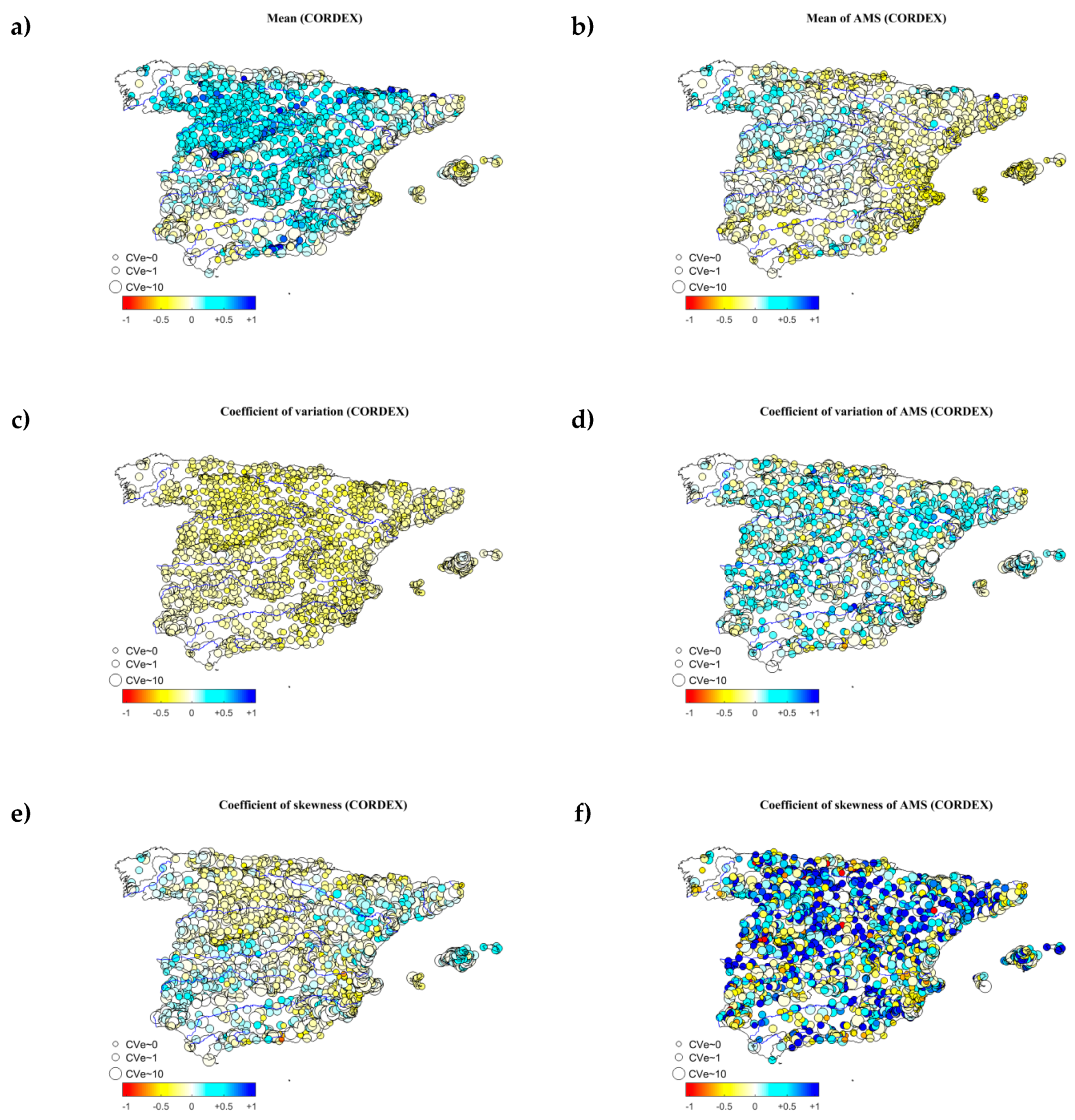
Figure 1 shows the results for the statistics described in Section 2.2.1, characterizing the errors between climate model projections in the control period and observation at rain-gauging sites in the same period. Each circle represents a gauging station. Its color represents the average error in the 12 climate models, and its size the dispersion of error values among climate models (CVe). The legend shows only three values of CVe for the sake of visual simplicity. The lowest value (CVe ~ 0) indicates that the 12 climate models have the same error (ei) for a given statistic (si), while the highest value (CVe ~ 10) means that climate models have differing error values with a large dispersion.
Figure 1 points out that climate models present a relatively good fit to observations, mainly for AMS. For daily series, Mean shows a generalized overestimation of mean daily precipitations (Figure 1a), especially in mountainous areas, while CV displays a smaller dispersion than observations (Figure 1c), indicating that climate models simulate daily precipitations with a more uniform pattern than observations. The smallest errors are found in MeanMax (Figure 1b) and CS (Figure 1e). Despite the light colors of the circles, most of them have CV evalues equal to one meaning that the statistic differs among climate models significantly. However, this result is reasonable when comparing such a huge amount of data produced with different parametrizations. Finally, CSmax results present a significant randomness (Figure 1f), showing the large uncertainty of climate models for simulating the most extreme values of precipitation. Such randomness is partially associated with the expected variability in third-order statistic estimates with short samples.
3.2. Expected Changes in Precipitation Quantilesin the Future
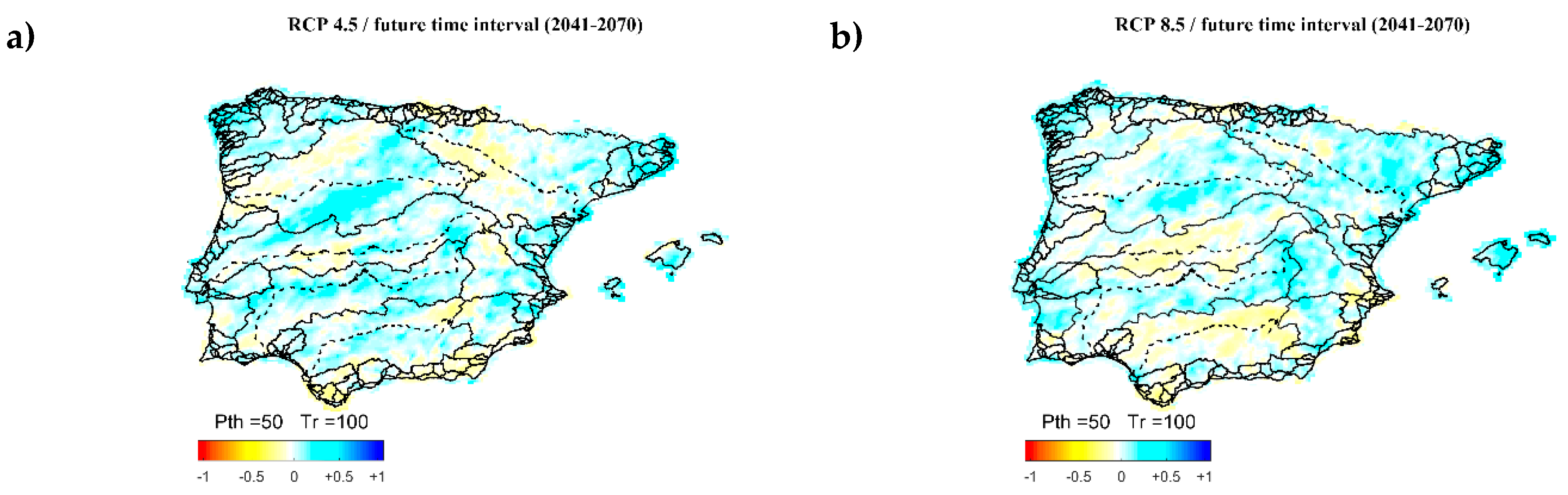
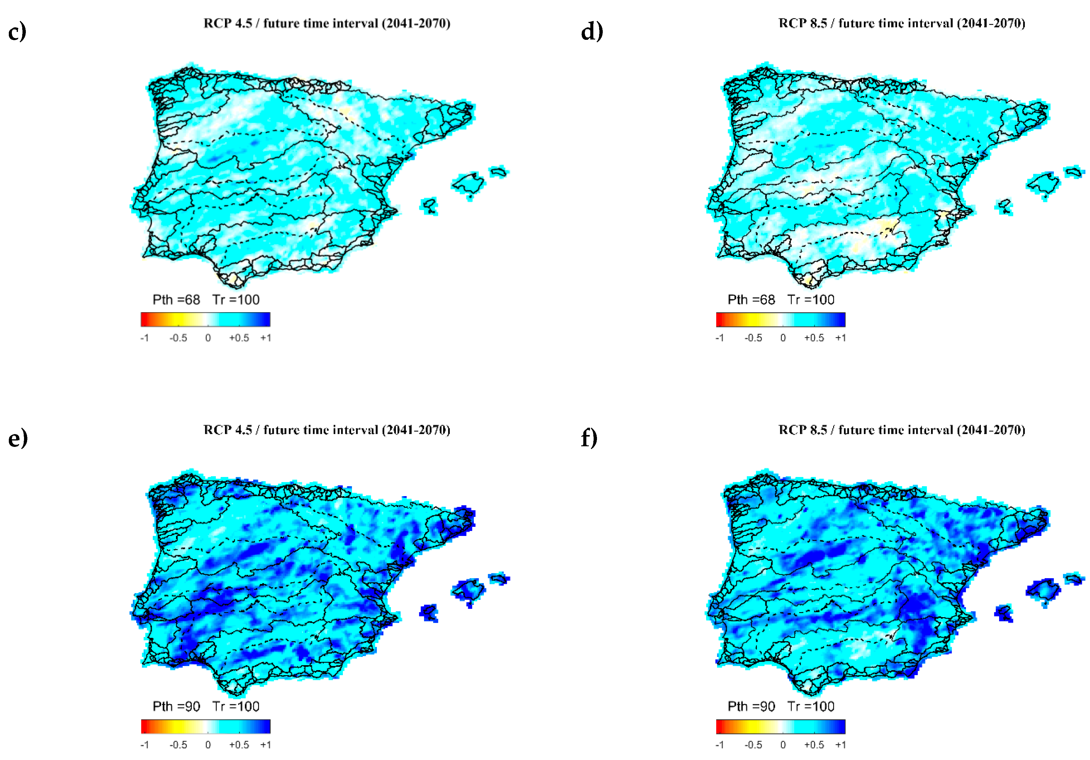
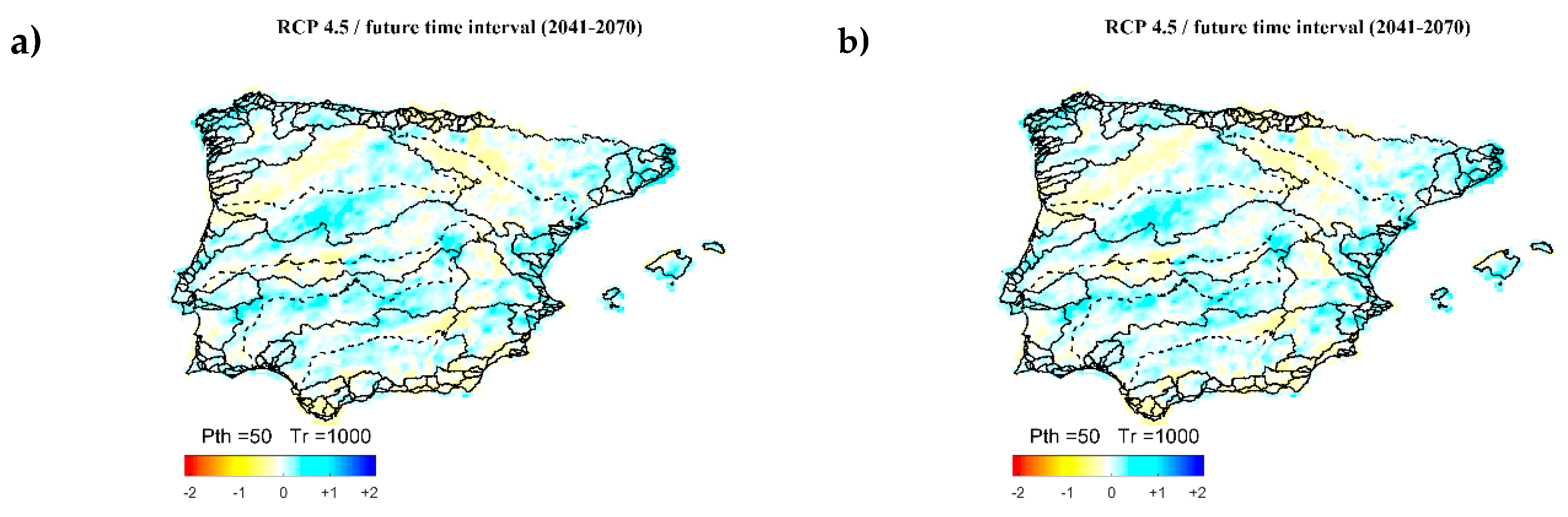
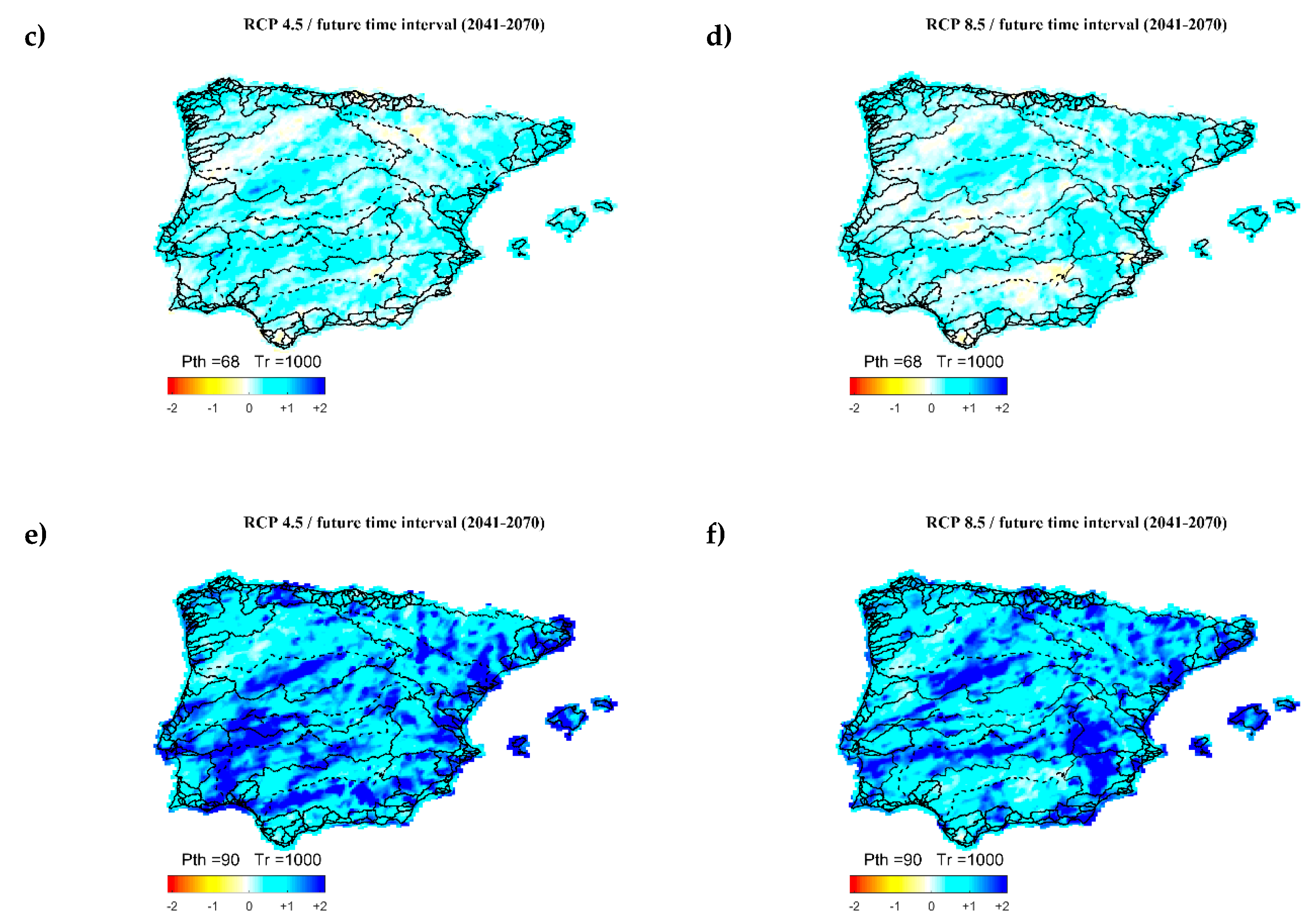
Figure 2, Figure 3 and Figure 4 show the delta changes (ΔT) in the 10-, 100-, and 1000-year precipitation quantiles, respectively, in the period 2041–2070 for both RCPs. Delta changes are shown for the 50th, 68th, and 90th percentiles. The median (50th percentile) offers an average change projected by climate models. It can be considered the most likely change that is expected to occur in the future, as half models project changes larger than the median and the other half smaller than the median. Higher percentiles identify the areas where larger changes may occur, especially the 90th percentile. The relative changes (ΔT) presented in the figures can be multiplied to obtain percentages of change. For example, a relative value ΔT = +0.25 (cyan) means a 25% increase in precipitation quantiles.
The figures for the periods 2011–2050 and 2071–2100, as well as the rest of return periods considered, can be found in the Supplementary Material. For the sake of simplicity, only the results shown in Figure 2, Figure 3 and Figure 4 are commented on.
Figure 2 shows that the main changes for the 10-year precipitation quantiles are located in both northeastern and northwestern corners of the Iberian Peninsula with increases around 20% for the 50th percentile. In the southern part of the Iberian Peninsula some decreases in precipitation quantiles are expected for the 50th percentile. Despite this similarity in the previous areas, the two RCPs considered show differing results, mainly in the southwestern and eastern parts of the Iberian Peninsula. RCP 8.5 shows a generalized increase and decrease over such areas, respectively. However, RCP 4.5 projects smaller and fuzzier changes. In addition, RCP 8.5 shows an increase in the 10-year precipitation quantiles in the Ebro River Basin, mainly in its center and northeastern corner, though RCP 4.5 shows a decrease. Summarizing, areas where the 10-year precipitation quantiles are expected to have the largest changes in both RCPs are the northeastern and northwestern corners of the Peninsula, the left side of the Douro River Basin, and the Balearic Islands. Results for 10-year precipitation quantile changes shown in Figure 2 may be useful for design and maintenance of sewage systems, as well as for flood risk plans in municipalities.
Results for higher return periods are shown in Figure 3 and Figure 4. Some patterns can be extracted, though quantile estimates for high return periods have large uncertainties considering the short time series considered. In general, results show a higher spatial variability in delta changes. Both northeastern and northwestern corners of the Iberian Peninsula show increases in precipitation quantiles, similar to the results obtained for the 10-year return period. However, the generalized increasing pattern in the Douro River Basin is less clear, as the return period increases, reducing such pattern to the left side of the basin. In addition, the Tagus and Guadiana River Basins show decreases and increases in precipitation quantiles, respectively, as the return period increases. Such patterns are evident for both RCPs. Large changes in such quantiles are also found in the left side of the Douro River Basin and the northeastern and northwestern corners of the Iberian Peninsula, though being less evident in the latter. Finally, the Mediterranean area and Balearic Islands could expect the largest changes for high precipitation quantiles, as opposed to the results for 10-year precipitation quantile. Results for 100-year precipitation quantiles presented in Figure 3 may be useful for flood risk management plans at the catchment scale. In addition, expected changes in 1000-year precipitation quantiles shown in Figure 4 may be useful for critical infrastructures, such as dams.
Table 3 and Table 4 summarize the results shown in Figure 2, Figure 3 and Figure 4, Supplementary Material, and results for other return periods. The Iberian Peninsula and the Balearic Islands were divided into 13 regions, by either boundaries of the river basin authorities or merging coastal basins with similar climatic characteristics. The geographical distribution of the regions can be seen in Figure 5, with different colors assigned for each region. The tables show qualitative expected changes. The green color represents a generalized positive change in the region (increase in the precipitation quantile). Red color indicates a generalized negative change in the region (decrease in the precipitation quantile). The orange color represents regions where both changes appear, and finally, no color was assigned to regions where the change is not seen clearly or there is no change.
3.3. Uncertainty of Delta Changes in Precipitation Quantiles
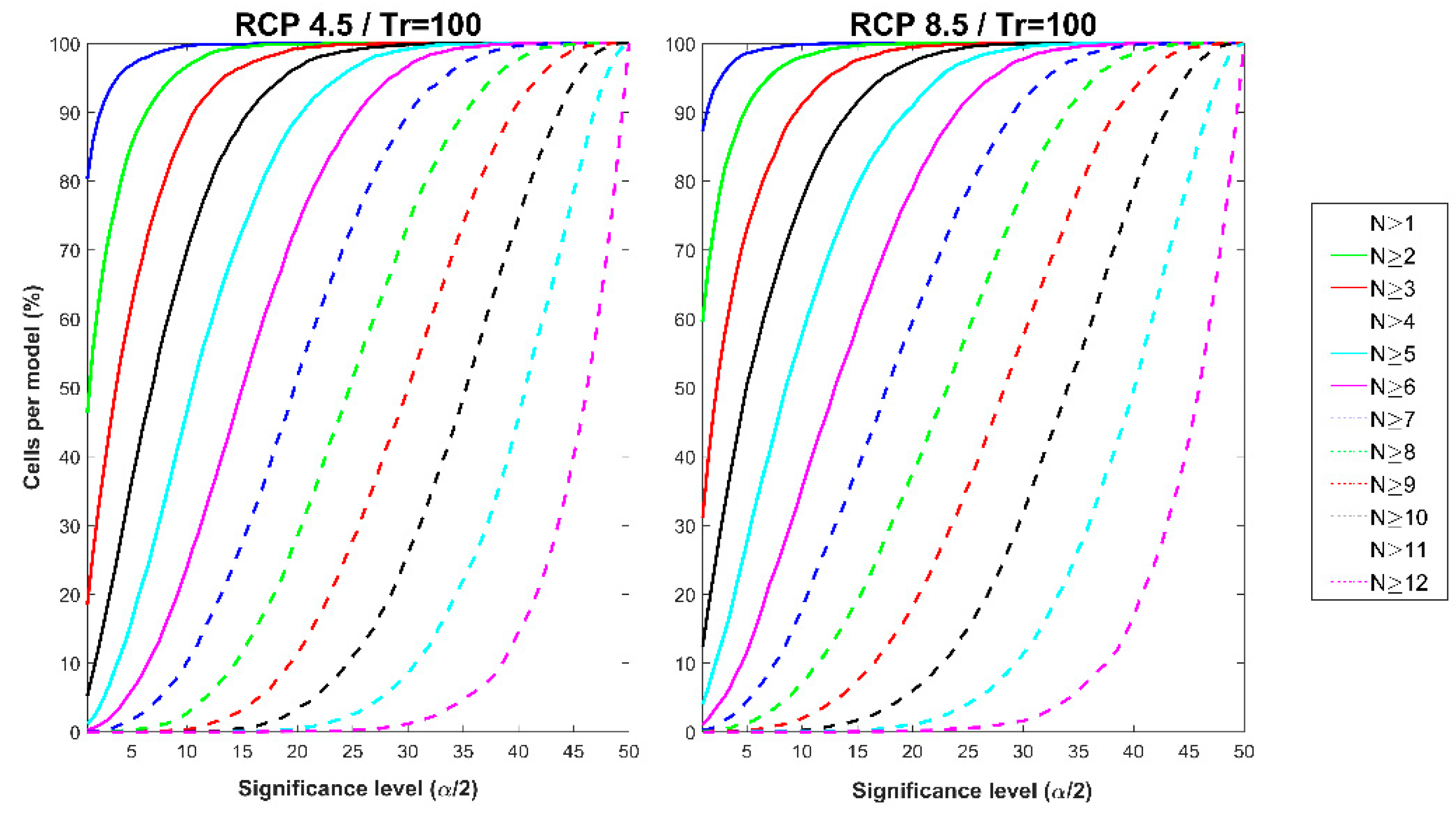
In order to identify appropriate significance thresholds, the influence of both the two-sided significance level (α) and the minimum number of models with change (N) in the results was examined. Figure 6 shows the average percentage of cells per climate model with significant changes against the significance threshold, drawn as one-sided (α/2). Each line represents a given minimum number of models with change (N). The analysis was conducted for the 100-year precipitation quantile in the period 2041–2070, as similar results were found for other return periods and periods in the future.
The comparison between both RCPs shows that the behavior is similar for all the minimum number of climate models with significant changes, though a small favorable shift in the percentage of cells per model in the RCP 4.5 can be seen. For N ≥ 1 (at least one model with significant changes), the average number of cells per model reaches almost 90% with a significance level of 5%. However, a significance level of 50% is needed to reach the same percentage of cells for N ≥ 12. Furthermore, the distributions of the different minimum number of models are equidistant. Thus, no clear hint arises from the evaluation.
3.4. Spatial Layout of Significant Changes
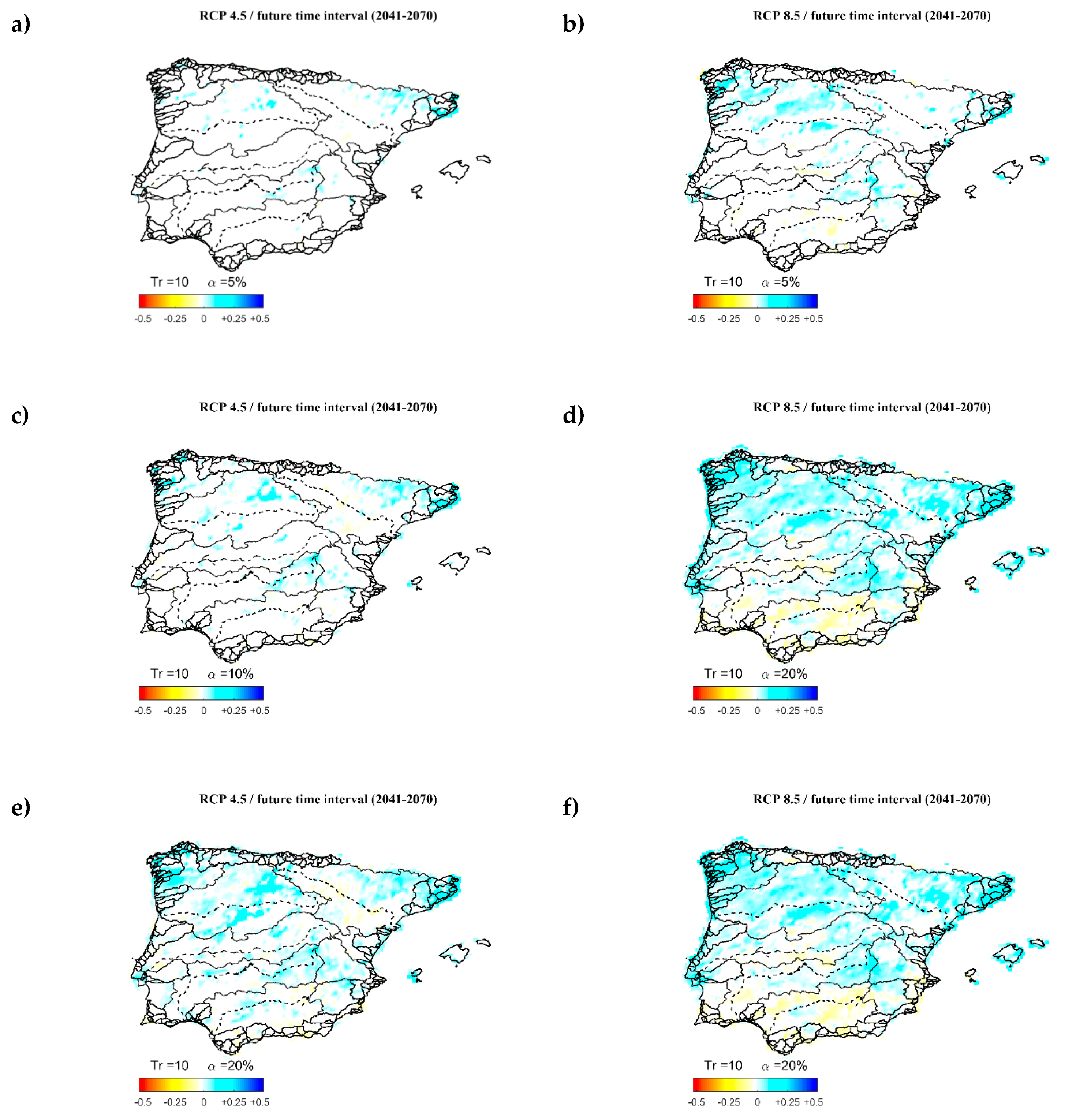
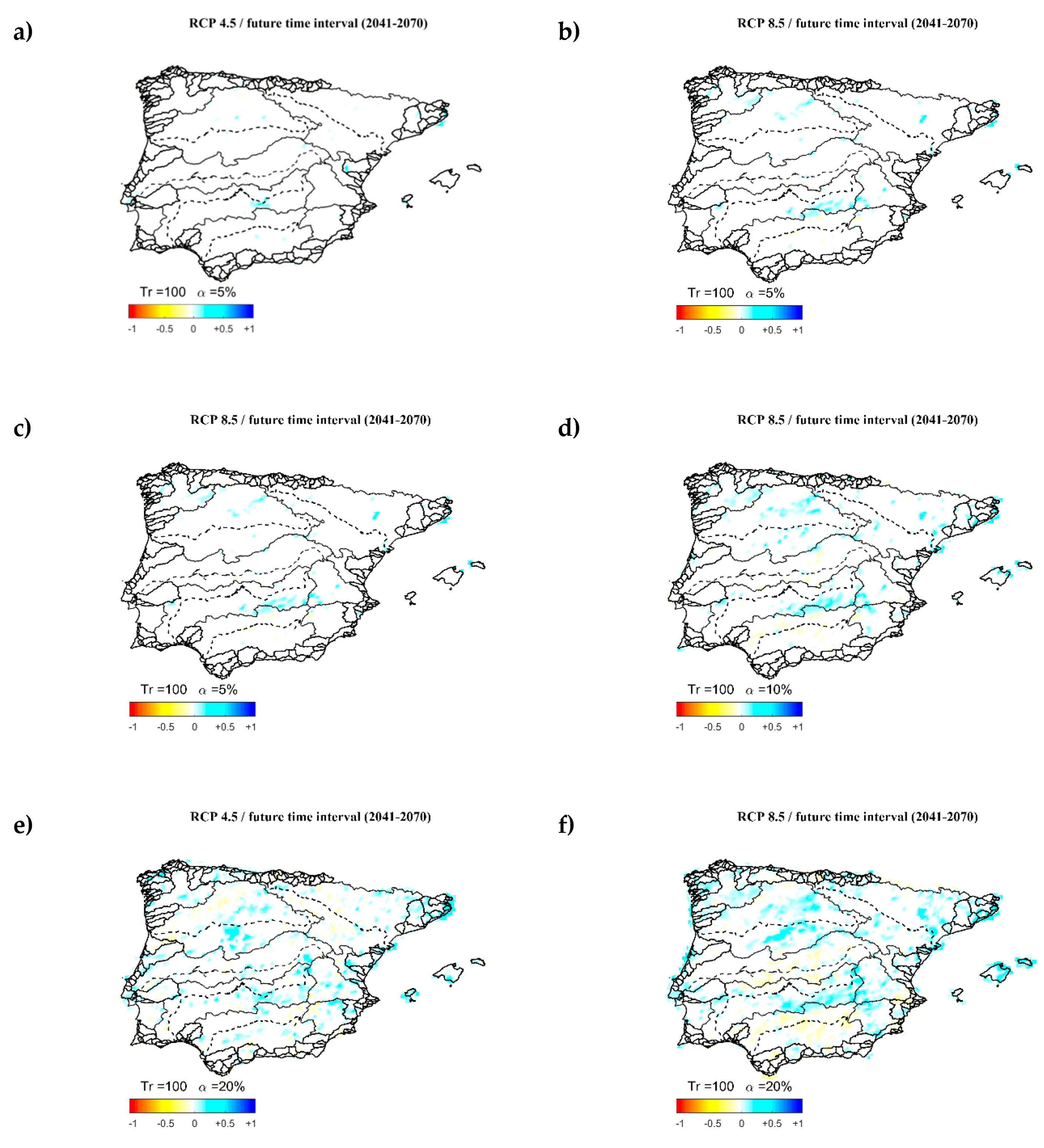
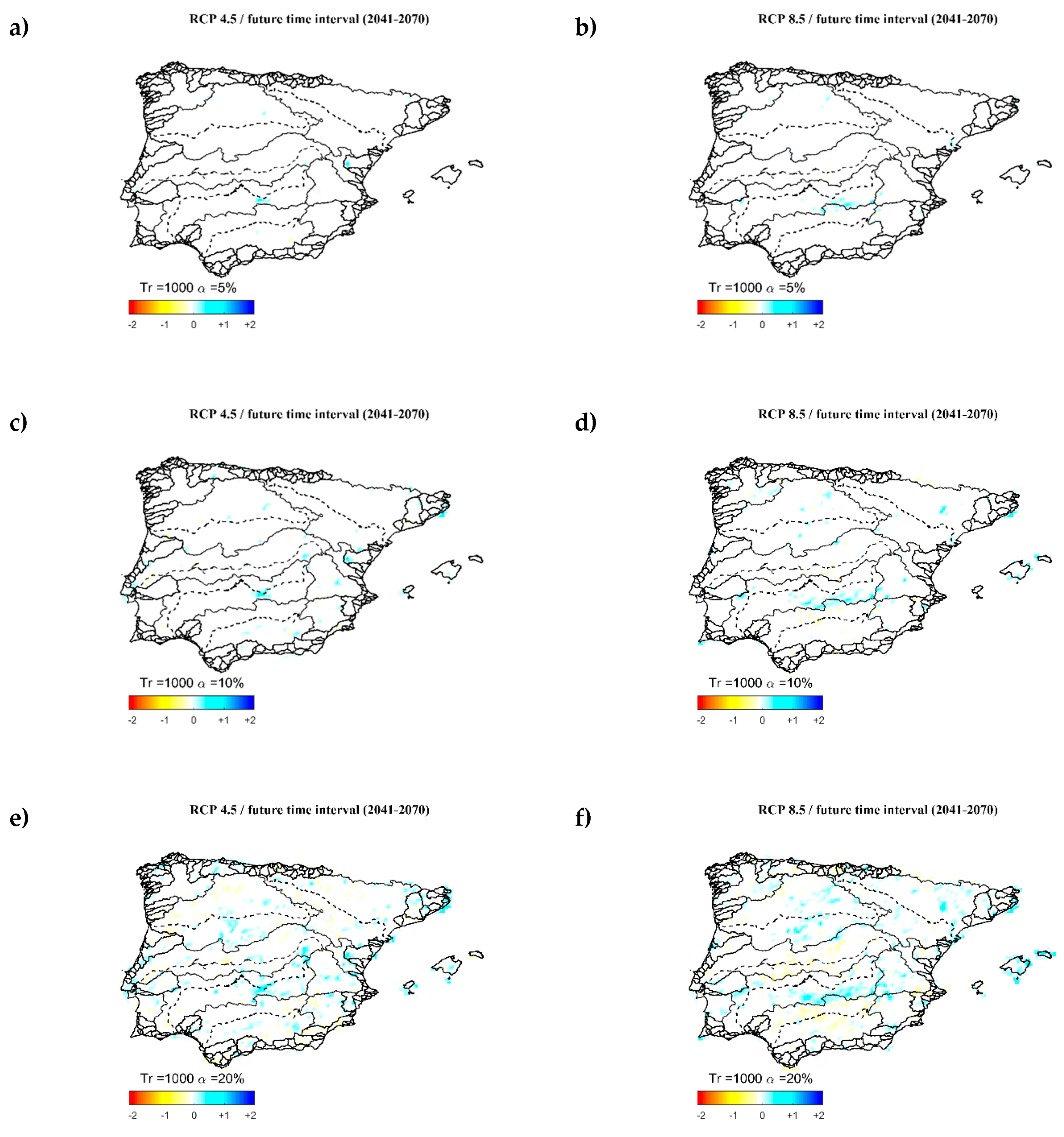
Spatial distribution of cells with significant changes for a set of thresholds and return periods are outlined in Figure 7, Figure 8 and Figure 9, in order to explore further about the selection of the significant thresholds. A minimum number of models with change larger than or equal to six (N ≥ 6) was selected, as it means that at least half of the climate models have a significant change. The 10-, 100-, and 1000-year precipitation quantiles were selected, considering the period 2041–2070. Three thresholds of interest were considered: 5%, 10%, and 20% two-sided significance levels. The rest of the future periods and precipitation quantiles can be found in Supplementary Material. In order to present the results, the same smoothing procedure used in Section 4.1 was adopted.
As expected, the higher the significance level, the larger the number of cells that are significant. Furthermore, Figure 7, Figure 8 and Figure 9 show that more cells with a significant change are identified in RCP 8.5 than RCP 4.5, for all thresholds. In general, despite some zones, both RCPs present similar change signs. However, RCP 8.5 shows more areas with negative changes than RCP 4.5, especially in the center of Tagus and Guadalquivir River Basins. Besides, as the return period rises, the number of significant cells decreases. However, results for the 100-year and 1000-year precipitation quantiles are similar, although results differ for the 10-year quantile.
Considering significance thresholds, areas with significant changes have the same sign for both RCPs, despite the results obtained in Section 3.2 that showed that the change sign varied depending on the RCP considered. For example, in the left side of Douro and Guadiana River Basins, a small cyan zone can be seen for both RCP and quantiles. This suggests that real significant changes can be seen in both RCPs.
In this study, spatial correlation among significant changes was not considered. Consequently, smaller significance levels (5%) could show smaller extents than expected. Larger areas with significant changes obtained for higher significance levels (20%) point to such larger extents of expected changes. Therefore, high significance levels may be recommended.
4. Discussion and Conclusions
4.1. Model Biases
The first step in the assessment of precipitation projections supplied by climate models consists of calculating biases in the control period, in order to check if climate models can reproduce actual climate conditions in the past. A comparison between climate projections and observations in the control period was conducted in the Spanish Iberian Peninsula and the Balearic Islands, using observed data available at 1742 rain-gauging sites.
Statistics for daily series show some areas with an overestimation in the mean daily precipitation, especially for mountainous areas, as well as a generalized underestimation in its dispersion. However, more accurate results were found in simulating the coefficient of skewness.
Extreme precipitation events were studied through annual maximum series. Results show smaller errors in the mean and dispersion, while they show large errors spatially random for the coefficient of skewness.
Summarizing, climate models are able to reproduce statistical properties of annual maximum precipitation series better than daily precipitation series, mainly for characterizing mean values and dispersion.
4.2. Uncertainty Thresholds
The uncertainty analysis shows the complexity in selecting both thresholds considered. The significance level represents a threshold to consider a change as not driven by natural variability. The minimum number of climate models with a significant change describes the minimum number of climate models that must have a significant change in a cell to consider that the precipitation quantile in such cell is expected to change in the future.
Regarding the minimum number of climate models, the percentage of cells with change was plotted against the significance threshold, to compare different choices for the threshold. The results show equidistance between the distributions for the values of the considered threshold. Besides, similar results were found for both RCPs. Therefore, a trade-off option may be to consider a threshold equal to at least half of the total number of climate models, which in this case is six. A higher number of climate models leads to a higher significance threshold to obtain changes, especially when more than eight models is considered.
The choice of the significance threshold depends on the scientific rigor required. A 1% threshold leads to almost no cells with significant changes. However, Figure 7, Figure 8 and Figure 9 show that with a 10% significance level, some more areas with significant changes emerge, even for the highest return period quantiles. Thus, a threshold between 1% and 20% may be reasonable for climatic studies. In addition, cross spatial correlation among significant changes was not considered in this study. Consequently, a higher significance level could be considered reasonable.
4.3. General and Significant Changes in Precipitation Quantiles
The expected changes in annual maximum daily precipitation quantiles were assessed in the Iberian Peninsula and the Balearic Islands. Identified changes depend not only on the geographical location, but also on the RCP, precipitation quantile, and period considered, as the results may indicate that climate oscillates over time.
Despite such spatiotemporal dispersion in the results, some general trends were found. First, Table 3 and Table 4 show that a general decrease pattern in both low and high return periods is expected in the Guadalquivir River and Southern Basins. Decreases were also found in some inland parts of the Iberian Peninsula, such as the Tagus River Basin and some areas of the Ebro River Basin, especially for high return periods. Second, significant increases were found in the northern part of the Iberian Peninsula, both in the Douro River Basin and some areas of the Ebro River Basin, as well as the upper eastern and western corners (Catalonia and Galicia, respectively), with large changes in some return periods. Therefore, a clear north-south pattern was found. An increase in the precipitation quantiles are expected in northern areas, while a decrease is expected in southern parts of the Iberian Peninsula.
Regarding the uncertainty analysis, some changes with respect to the previous results are highlighted. As it was expected, spatial extension of areas with change increases, as the significance threshold also increases. However, though the spatial extent of the change increases, the areas of change remain among levels of significance. Therefore, regional change patterns were found.
Areas with positive changes in both RCPs are the headwaters of the Guadiana River Basin, the central part of the Douro River Basin, and some specific areas of the Mediterranean coast. In addition, for high return period quantiles (100- to 1000-years), the Balearic Islands show such upward shift. Negative changes can be found in the Tagus River Basin and southeastern parts of Spain for RCP 8.5. Such negative trend agrees with the findings of [9]. Nevertheless, this study found larger areas with positive changes in that region than those obtained from [9].
Finally, areas with significant changes are usually identified in both RCPs, regardless of the threshold and quantile considered. Therefore, a similar sign of change for both RCPs in a given area could indicate that such change is likely to happen in the future.
5. Patents
The findings of this study are collected in the database ‘Tasas de cambio en los cuantiles de precipitación diaria máxima anual esperables en situación de cambio climático a escala nacional’ that was registered in the ‘Registro Territorial de la Propiedad Intelectual de la Comunidad de Madrid’ (Spain) on 12 March 2018 with the code 16/2018/5074.
Supplementary Materials
The following are available online at https://www.mdpi.com/2073-4441/11/11/2375/s1. Figures S1–S7: Relative changes (ΔT) for the T-year precipitation quantiles expected in the period 2011–2040. The left column shows results for the RCP 4.5 and the right column for the RCP 8.5. The first row shows results for the 50th percentile, the second row for the 68th percentile, and the third row for the 90th percentile. The colorbar in the lower left corner indicates the color associated to the percentage of change. Blue colors indicate increases in precipitation quantiles and red colors decreases. (S1—T = 2; S2—T = 5; S3—T = 10; S4—T = 50; S5—T = 100; S6—T = 500; S7—T = 1000). Figures S8–S11: Relative changes (ΔT) for the T-year precipitation quantiles expected in the period 2041–2070. The left column shows results for the RCP 4.5 and the right column for the RCP 8.5. The first row shows results for the 50th percentile, the second row for the 68th percentile, and the third row for the 90th percentile. The colorbar in the lower left corner indicates the color associated to the percentage of change. Blue colors indicate increases in precipitation quantiles and red colors decreases. (S8—T = 2; S9—T = 5; S10—T = 50; S11—T = 500). Figures S12–S18: Relative changes (ΔT) for the T-year precipitation quantiles expected in the period 2071–2095. The left column shows results for the RCP 4.5 and the right column for the RCP 8.5. The first row shows results for the 50th percentile, the second row for the 68th percentile, and the third row for the 90th percentile. The colorbar in the lower left corner indicates the color associated to the percentage of change.Blue colors indicate increases in precipitation quantiles and red colors decreases. (S12—T = 2; S13—T = 5; S14—T = 10; S15—T = 50; S16—T = 100; S17—T = 500; S18—T = 1000).Figures S19–S25: Spatial distribution of significant changes in the T-year precipitation quantile and period 2011–2040, with a significant two-sided level (α) of 5% (a,b), 10% (c,d), and 20% (e,f). The left column shows the results for RCP 4.5 and the right column for RCP 8.5. A minimum number of six models with significant changewas considered. (S19—T = 2; S20—T = 5; S21—T = 10; S22—T = 50; S23—T = 100; S24—T = 500; S25—T = 1000).Figures S26–S29: Spatial distribution of significant changes in the T-year precipitation quantile and period 2041–2070, with a significant two-sided level (α) of 5% (a,b), 10% (c,d), and 20% (e,f). The left column shows the results for RCP 4.5 and the right column for RCP 8.5. A minimum number of six models with significant changewas considered. (S26—T = 2; S27—T = 5; S28—T = 50; S29—T = 500). Figures S30–S36: Spatial distribution of significant changes in the T-year precipitation quantile and period 2071–2095, with a significant two-sided level (α) of 5% (a,b), 10% (c,d), and 20% (e,f). The left column shows the results for RCP 4.5 and the right column for RCP 8.5. A minimum number of six models with significant changewas considered. (S30—T = 2; S31—T = 5; S32—T = 10; S33—T = 50; S34—T = 100; S35—T = 500; S36—T = 1000).
Author Contributions
Both Authors were involved in conceptualization, data acquisition, and methodology formulation. C.G. was the main producer and writer of the work done, while L.M. was responsible for reviewing and editing the article.
Funding
This research was funded by the Spanish Ministry of Economy and Competitiveness, through the project CGL2014-52570-R ‘Impact of climate change on the bivariate flood frequency curve’.
Acknowledgments
The authors acknowledge the Spanish Centre of Hydrographic Studies of CEDEX, the AgenciaEstatal de Meteorología (AEMET) and the CORDEX initiative, especially the EURO-CORDEX project, for providing climate and hydrological data used in this paper. The authors acknowledge that this study was supported by the project CGL2014-52570-R ‘Impact of climate change on the bivariate flood frequency curve’ of the Spanish Ministry of Economy and Competitiveness.
Conflicts of Interest
The authors declare no potential conflict of interest.
References
- Beniston, M.; Stephenson, D.B.; Christensen, O.B.; Ferro, C.A.T.; Frei, C.; Goyette, S.; Halsnaes, K.; Holt, T.; Jylhä, K.; Koffi, B.; et al. Future extreme events in European climate: An exploration of regional climate model projections. Clim. Chang. 2007, 81, 71–95. [Google Scholar] [CrossRef]
- Prein, A.F.; Gobiet, A.; Truhetz, H.; Keuler, K.; Goergen, K.; Teichmann, C.; Fox Maule, C.; van Meijgaard, E.; Déqué, M.; Nikulin, G.; et al. Precipitation in the EURO-CORDEX 0.11° and 0.44° simulations: High resolution, high benefits? Clim. Dyn. 2016, 46, 383–412. [Google Scholar] [CrossRef]
- Mascaro, G.; Viola, F.; Deidda, R. Evaluation of precipitation from EURO-CORDEX regional climate simulations in a small-scale Mediterranean site. J.Geophys. Res. Atmos. 2018, 123, 1604–1625. [Google Scholar] [CrossRef]
- Casanueva, A.; Kotlarski, S.; Herrera, S.; Fernández, J.; Gutiérrez, J.M.; Boberg, F.; Colette, A.; Christensen, O.B.; Goergen, K.; Jacob, D.; et al. Daily precipitation statistics in a EURO-CORDEX RCM ensemble: Added value of raw and bias-corrected high-resolution simulations. Clim. Dyn. 2016, 47, 719–737. [Google Scholar] [CrossRef]
- Frei, C.; Christensen, J.H.; Déqué, M.; Jacob, D.; Jones, R.G.; Vidale, P.L. Daily precipitation statistics in regional climate models: Evaluation and intercomparison for the European Alps. J. Geophys. Res. 2003, 108, 4124. [Google Scholar] [CrossRef]
- Jacob, D.; Bärring, L.; Christensen, O.B.; Christensen, J.H.; de Castro, M.; Déqué, M.; Giorgi, F.; Hagemann, S.; Hirschi, M.; Jones, R.; et al. An inter-comparison of regional climate models for Europe: Model performance in present-day climate. Clim. Chang. 2007, 81, 31–52. [Google Scholar] [CrossRef]
- Kotlarski, S.; Paul, F.; Jacob, D. Forcing a Distributed Glacier Mass Balance Model with the Regional Climate Model REMO. Part I: Climate Model Evaluation. J. Clim. 2010, 23, 1589–1606. [Google Scholar] [CrossRef]
- Kotlarski, S.; Keuler, K.; Christensen, O.B.; Colette, A.; Deque, M.; Gobiet, A.; Goergen, K.; Jacob, D.; Lüthi, D.; Meijgaard, E.V.; et al. Regional climate modelling on European scales: A joint standard evaluation of the EURO-CORDEX RCM ensemble. Geosci. Model Dev. Atmos. 2014, 7, 1297–1333. [Google Scholar] [CrossRef]
- Monjo, R.; Gaitán, E.; Pórtoles, J.; Ribalaygua, J.; Torres, L. Changes in extreme precipitation over Spain using statistical downscaling of CMIP5 projections. Int. J. Climatol. 2016, 36, 757–769. [Google Scholar] [CrossRef]
- Frei, C.; Schöll, R.; Fukutome, S.; Schmidli, J.; Vidale, P.L. Future change of precipitation extremes in Europe: Intercomparison of scenarios from regional climate models. J. Geophys. Res. 2006, 111, D06105. [Google Scholar] [CrossRef]
- Fowler, H.J.; Ekström, M.; Blenkinsop, S.; Smith, A.P. Estimating change in extreme European precipitation using a multimodel ensemble. J. Geophys. Res. 2007, 112, D18104. [Google Scholar] [CrossRef]
- Rajczak, J.; Pall, P.; Schär, C. Projections of extreme precipitation events in regional climate simulations for Europe and the Alpine Region. J. Geophys. Res. 2010, 118, 3610–3626. [Google Scholar] [CrossRef]
- Herrera, S.; Fita, L.; Fernández, J.; Gutiérrez, J.M. Evaluation of the mean and extreme precipitation regimes from the ENSEMBLES regional climate multimodel simulations over Spain. J. Geophys. Res. 2010, 115, D21117. [Google Scholar] [CrossRef]
- Giorgi, F.; Lionello, P. Climate change projections for the mediterranean region. Glob. Planet Chang. 2008, 63, 90–104. [Google Scholar] [CrossRef]
- Jacob, D.; Petersen, J.; Eggert, B.; Alias, A.; Christensen, O.B.; Bouwer, L.M.; Braun, A.; Colette, A.; Déqué, M.; Georgievski, G.; et al. EURO-CORDEX: New high-resolution climate change projections for European impact research. Reg. Environ. Chang. 2014, 14, 563–578. [Google Scholar] [CrossRef]
- Hosking, J.R.M.; Wallis, J.R.; Wood, E.F. Estimation of the generalized extreme-value distribution by the method of probability-weighted moments. Technometrics 1985, 27, 251–261. [Google Scholar] [CrossRef]
- Svensson, C.; Jones, D.A. Review of rainfall frequency estimation methods. J. Flood Risk Manag. 2010, 3, 296–313. [Google Scholar] [CrossRef] [Green Version]
- Ferrer, J.; Ardiles, L. Análisis estadístico de las series anuales de máximas lluvias diarias en España. Ing. Civ. 1994, 95, 87–100. [Google Scholar]
Figure 1.
Average errors between observations at each gauging station and CORDEX climate model projections in the control period. The first column shows statistics for daily series. The second column shows statistics for the annual maximum series (AMS) series. (a) Mean; (b) MeanMax; (c) CV; (d) CVMax; (e) CS; (f) CSMax. Colors of the circles represent the magnitude of the average error of the 12 climate models. Circle size represents the dispersion of errors among climate models through CVe.

Figure 2.
Relative changes (ΔT) for the 10-year precipitation quantiles expected in the period 2041–2070. The left column shows the results for the RCP4.5 (a,c,e) and the right column for the RCP 8.5 (b,d,f). The first row shows the results for the 50th percentile (a,b), the second row for the 68th percentile (c,d), and the third row for the 90th percentile (e,f). The colorbar in the lower left corner indicates the color associated to the percentage of change. Blue colors indicate increases in precipitation quantiles and red colors decreases.

Figure 3.
Relative changes (ΔT) for the 100-year precipitation quantiles expected in the period 2041–2070. The left column shows results for the RCP 4.5 (a,c,e) and the right column for the RCP 8.5 (b,d,f). The first row shows results for the 50th percentile (a,b), the second row for the 68th percentile (c,d), and the third row for the 90th percentile (e,f). The colorbar in the lower left corner indicates the color associated to the percentage of change. Blue colors indicate increases in precipitation quantiles and red colors decreases.


Figure 4.
Relative changes (ΔT) for the 1000-year precipitation quantiles expected in the period 2041–2070. The left column shows results for the RCP 4.5 (a,c,e) and the right column for the RCP 8.5 (b,d,f). The first row shows results for the 50th percentile (a,b), the second row for the 68th percentile (c,d), and the third row for the 90th percentile (e,f). The colorbar in the lower left corner indicates the color associated to the percentage of change. Blue colors indicate increases in precipitation quantiles and red colors decreases.


Figure 5.
Geographic location of the regions considered in the study.

Figure 6.
Distribution of the average percentage of cells with significant changes per climate model for the 100-year precipitation quantile in the period 2041–2070, considering varying significance levels (α/2): left column RCP 4.5; right column RCP 8.5. Each curve represents a minimum number of models with a significant change (N; from 1 to 12). The significance threshold shown in the x-axis represents the one-sided threshold (α/2).

Figure 7.
Spatial distribution of significant changes in the 10-year precipitation quantile and period 2041–2070, with a significant two-sided level (α) of 5% (a,b), 10% (c,d), and 20% (e,f). The left column shows the results for RCP 4.5 and the right column for RCP 8.5. A minimum number of six models with significant change was considered.

Figure 8.
Spatial distribution of significant changes in the 100-year precipitation quantile and period 2041–2070, with a significant two-sided level (α) of 5% (a,b), 10% (c,d), and 20% (e,f). The left column shows the results for RCP 4.5 and the right column for RCP 8.5. A minimum number of six models with significant change was considered.

Figure 9.
Spatial distribution of significant changes in the 1000-year precipitation quantile and period 2041–2070, with a significant two-sided level (α) of 5% (a,b), 10% (c,d), and 20% (e,f). The left column shows the results for RCP 4.5 and the right column for RCP 8.5. A minimum number of six models with significant change was considered.


Table 1.
Climate models used in the study.
| ID | Acronym | GCM | RCM | Simulation Periods (Control/Future) |
|---|---|---|---|---|
| 1 | ICH-CCL | ICHEC-EC-EARTH | CCLM4-8-17 | 1951–2005/2006–2100 |
| 2 | MPI-CCL | MPI-ESM-LR | CCLM4-8-17 | 1951–2005/2006–2100 |
| 3 | MOH-RAC | MOHC-HadGEM2-ES | RACMO22E | 1951–2005/2006–2099 |
| 4 | CNR-CCL | CNRM-CM5 | CCLM4-8-17 | 1951–2005/2006–2100 |
| 5 | ICH-RAC | ICHEC-EC-EARTH | RACMO22E | 1951–2005/2006–2100 |
| 6 | MOH-CCL | MOHC-HadGEM2-ES | CCLM4-8-17 | 1951–2005/2006–2099 |
| 7 | IPS-WRF | IPSL-CM5A-MR | WRF331F | 1951–2005/2006–2100 |
| 8 | IPS-RCA | IPSL-CM5A-MR | RCA4 | 1971–2005/2006–2100 |
| 9 | MOH-RCA | MOHC-HadGEM2-ES | RCA4 | 1971–2005/2006–2099 |
| 10 | ICH-RCA | ICHEC-EC-EARTH | RCA4 | 1971–2005/2006–2100 |
| 11 | CNR-RCA | CNRM-CM5 | RCA4 | 1971–2005/2006–2100 |
| 12 | MPI-RCA | MPI-ESM-LR | RCA4 | 1971–2005/2006–2100 |
Table 2.
Statistics used to compare observations with simulations of climate models in the control period.
Table 2.
Statistics used to compare observations with simulations of climate models in the control period.
| Statistic | Abbreviation |
|---|---|
| Mean | Mean |
| Coefficient of variation | CV |
| Coefficient of skewness | CS |
| Mean of AMS | MeanMax |
| Coefficient of variation of AMS | CVMax |
| Coefficient of skewness of AMS | CSMax |
Table 3.
Expected changes in precipitation quantiles for RCP 4.5 in the regions considered. For each return period, the first column shows the period 2011–2040, the second column the period 2041–2070, and the third column the period 2071–2095.
Table 3.
Expected changes in precipitation quantiles for RCP 4.5 in the regions considered. For each return period, the first column shows the period 2011–2040, the second column the period 2041–2070, and the third column the period 2071–2095.
| RCP | 4.5 | ||||||||||||||||||||
|---|---|---|---|---|---|---|---|---|---|---|---|---|---|---|---|---|---|---|---|---|---|
| Return Period | 2 | 5 | 10 | 50 | 100 | 500 | 1000 | ||||||||||||||
| Future Time Interval | 11–40 | 41–70 | 71–95 | 11–40 | 41–70 | 71–95 | 11–40 | 41–70 | 71–95 | 11–40 | 41–70 | 71–95 | 11–40 | 41–70 | 71–95 | 11–40 | 41–70 | 71–95 | 11–40 | 41–70 | 71–95 |
| Upper Mediterranean Basins | + | + | + | + | + | + | +/− | + | + | + | + | + | + | + | + | ||||||
| EbroRiver Basin | +/− | +/− | + | +/− | +/− | + | +/− | +/− | + | +/− | +/− | +/− | +/− | +/− | +/− | +/− | +/− | − | +/− | +/− | |
| Northern Basins | − | − | + | + | + | + | + | + | +/− | +/− | + | +/− | + | ||||||||
| Northwestern Basins and Miño-Sil River Basin | + | + | + | + | + | + | + | + | + | + | + | + | + | − | + | − | + | ||||
| Douro River Basin | + | + | + | + | + | + | + | + | + | + | +/− | + | + | +/− | + | +/− | +/− | + | +/− | +/− | + |
| Tagus River Basin | + | + | + | + | +/− | + | +/− | − | + | − | − | +/− | − | − | +/− | − | − | − | |||
| Atlantic Basins | + | + | +/− | + | +/− | + | − | − | |||||||||||||
| Guadiana River Basin | − | − | + | +/− | + | +/− | + | + | + | + | +/− | + | +/− | +/− | + | +/− | + | + | +/− | ||
| Guadalquivir River Basin | − | +/− | + | +/− | + | +/− | + | + | +/− | + | + | + | + | − | + | + | − | + | + | ||
| Southern Basins | − | − | − | − | − | − | − | +/− | − | − | − | − | − | − | − | − | |||||
| Segura and Jucar River Basins | − | +/− | +/− | − | + | + | − | + | + | − | + | + | + | + | +/− | + | +/− | − | + | +/− | |
| Mediterranean Basins | − | − | − | + | + | +/− | + | − | + | +/− | + | ||||||||||
| Balearic Islands | − | + | − | + | + | + | +/− | + | +/− | +/− | + | +/− | + | ||||||||
Notes: green—Most of the region increases its precipitation; orange—Both signs (increase and decrease) appeared; red—Most of the region decreases its precipitation; blank—No sign has appeared.
Table 4.
Expected changes in precipitation quantiles for RCP 8.5 in the regions considered. For each return period, the first column shows the period 2011–2040, the second column the period 2041–2070, and the third column the period 2071–2095.
Table 4.
Expected changes in precipitation quantiles for RCP 8.5 in the regions considered. For each return period, the first column shows the period 2011–2040, the second column the period 2041–2070, and the third column the period 2071–2095.
| RCP | 8.5 | ||||||||||||||||||||
|---|---|---|---|---|---|---|---|---|---|---|---|---|---|---|---|---|---|---|---|---|---|
| Return Period | 2 | 5 | 10 | 50 | 100 | 500 | 1000 | ||||||||||||||
| Future Time Interval | 11–40 | 41–70 | 71–95 | 11–40 | 41–70 | 71–95 | 11–40 | 41–70 | 71–95 | 11–40 | 41–70 | 71–95 | 11–40 | 41–70 | 71–95 | 11–40 | 41–70 | 71–95 | 11–40 | 41–70 | 71–95 |
| Upper Mediterranean Basins | + | + | + | + | + | + | + | + | + | + | + | + | + | + | +/− | + | + | + | + | ||
| EbroRiver Basin | +/− | + | +/− | +/− | + | + | +/− | + | + | +/− | + | + | +/− | + | +/− | +/− | +/− | +/− | − | +/− | +/− |
| Northern Basins | − | +/− | +/− | +/− | + | +/− | +/− | + | + | +/− | +/− | + | +/− | + | |||||||
| Northwestern Basins and Miño-Sil River Basin | + | + | + | + | + | + | + | + | + | +/− | + | + | +/− | + | + | +/− | +/− | + | +/− | +/− | + |
| Douro River Basin | + | + | + | + | + | + | + | + | + | + | + | + | + | + | + | +/− | +/− | + | + | +/− | + |
| Tagus River Basin | + | +/− | + | + | + | +/− | + | − | +/− | +/− | − | − | +/− | − | − | +/− | − | − | +/− | ||
| Atlantic Basins | +/− | +/− | +/− | +/− | +/− | + | + | +/− | + | + | + | + | − | + | + | − | + | ||||
| Guadiana River Basin | − | − | +/− | + | +/− | +/− | + | +/− | + | + | +/− | + | + | +/− | + | + | +/− | + | + | ||
| Guadalquivir River Basin | − | − | +/− | − | + | +/− | − | + | +/− | − | + | − | − | + | +/− | − | + | − | − | + | |
| Southern Basins | − | − | − | − | − | − | − | − | +/− | +/− | − | +/− | − | +/− | +/− | − | − | ||||
| Segura and Jucar River Basins | + | +/− | +/− | + | +/− | +/− | + | + | +/− | + | + | + | +/− | + | + | +/− | + | +/− | + | ||
| Mediterranean Basins | + | +/− | + | +/− | +/− | + | +/− | +/− | + | +/− | +/− | + | +/− | +/− | + | +/− | +/− | ||||
| Balearic Islands | + | − | + | + | + | + | + | + | +/− | + | + | +/− | + | + | +/− | + | + | + | + | ||
Notes: green—Most of the region increase its precipitation; orange—Both signs (increase and decrease) appeared; red—Most of the region decrease its precipitation; blank—No sign has appeared.
© 2019 by the authors. Licensee MDPI, Basel, Switzerland. This article is an open access article distributed under the terms and conditions of the Creative Commons Attribution (CC BY) license (http://creativecommons.org/licenses/by/4.0/).
Share and Cite
MDPI and ACS Style
Garijo, C.; Mediero, L. Assessment of Changes in Annual Maximum Precipitations in the Iberian Peninsula under Climate Change. Water 2019, 11, 2375. https://doi.org/10.3390/w11112375
AMA Style
Garijo C, Mediero L. Assessment of Changes in Annual Maximum Precipitations in the Iberian Peninsula under Climate Change. Water. 2019; 11(11):2375. https://doi.org/10.3390/w11112375
Chicago/Turabian StyleGarijo, Carlos, and Luis Mediero. 2019. "Assessment of Changes in Annual Maximum Precipitations in the Iberian Peninsula under Climate Change" Water 11, no. 11: 2375. https://doi.org/10.3390/w11112375
Note that from the first issue of 2016, this journal uses article numbers instead of page numbers. See further details here.