Impact of Climate Change on Water Balance Components and Droughts in the Guajoyo River Basin (El Salvador)


Department of Civil Engineering, Catholic University of San Antonio, Campus de los Jerónimos s/n, Guadalupe, 30107 Murcia, Spain
*
Author to whom correspondence should be addressed.
Water 2019, 11(11), 2360; https://doi.org/10.3390/w11112360
Submission received: 27 September 2019
/
Revised: 4 November 2019
/
Accepted: 8 November 2019
/
Published: 11 November 2019
(This article belongs to the Special Issue Modeling Global Change Impacts on Water Resources: Selected Papers from the 2019/2020 SWAT International Conferences)
Abstract
:This study assessed how changes in terms of temperature and precipitation might translate into changes in water availability and droughts in an area in a developing country with environmental interest. The hydrological model Soil and Water Assessment Tool (SWAT) was applied to analyze the impacts of climate change on water resources of the Guajoyo River Basin in El Salvador. El Salvador is in one of the most vulnerable regions in Latin America to the effects of climate change. The predicted future climate change by two climate change scenarios (RCP 4.5 and RCP 8.5) and five general circulation models (GCMs) were considered. A statistical analysis was performed to identify which GCM was better in terms of goodness of fit to variation in means and standard deviations of the historical series. A significant decreasing trend in precipitation and a significant increase in annual average temperatures were projected by the middle and the end of the twenty–first century. The results indicated a decreasing trend of the amount of water available and more severe droughts for future climate scenarios with respect to the base period (1975–2004). These findings will provide local water management authorities useful information in the face of climate change to help decision making.
1. Introduction
The last century has seen a dramatic increase in greenhouse gas emissions. These higher concentrations of carbon dioxide and other greenhouse gases in the Earth’s atmosphere increase the greenhouse effect and directly affect global temperature [1]. Consequently, global warming has caused higher evapotranspiration rates leading to changes in precipitation worldwide. Such global climate change significantly affects the hydrological cycle and streamflow regimes, especially at the basin scale [2], which directly affects ecosystems, water security and economic activity, mainly in the agricultural sector, in forestry and energy generation by hydroelectricity. Some of the consequences of climate change, such as an increase in extreme floods and droughts, maybe unavoidable [3]. Therefore, quantifying the climate change impact on water availability is essential to watershed management as well as to the formulation of adaptation strategies to mitigate its negative impacts [4].
According to the Intergovernmental Panel on Climate Change (IPCC) [5], it is expected that almost all regions of the world will experience a negative impact on climate change. Specifically, developing countries are more vulnerable to climate change than developed countries, due to increased exposure to extreme hydrometeorological events, the predominance of agriculture in their economies, poor infrastructure and less capital for developing adaptation measures [6,7]. This study explores local responses to climate change-related perturbations through one case study in a rural area of El Salvador, the Guajoyo River Basin. El Salvador is in one of the most vulnerable regions in Latin America to the effects of climate change, as it is located within a band of hurricanes and low-lying coastal areas, among other particularities [5,8]. Numerous publications have evaluated the impact of climate changes on the hydrological cycle in Latin America and the rest of the world. However, few studies focused on the evaluation of streamflow changes in El Salvador. Maurer et al. [9] studied the hydrologic impacts of climate change to the Lempa River Basin, one of the largest basins in Central America, covering portions of Guatemala, Honduras, and El Salvador. Imbach et al. [10] evaluated the likelihood and magnitude of the impacts of climate change on potential vegetation and the water cycle in El Salvador and the rest of Central America. Other studies that analyzed climate change near the study area, albeit without focusing on the study of water availability, were: Campos et al. [8] explored local adaptation strategies to mitigate climate change-related perturbations through two case studies in rural areas of Mexico and El Salvador; and Aguilar et al. [11] assessed climate vulnerability and adaptation to climate change of rural inhabitants in the central coastal plain of El Salvador.
Hydrological models are the principal tools used to explore the potential effects of climate change on water resources [12]. The hydrological model Soil and Water Assessment Tool (SWAT) has been successfully and widely used all over the world to simulate basin hydrology under different climate change scenarios [13,14,15]. However, to the best of our knowledge, no previous works have been found applying the SWAT model in El Salvador and so far no study has been carried out in the Guajoyo River Basin in relation to the impact of climate change on water resource availability under climate change conditions in particular.
The Guajoyo River Basin presents an environmental interest in terms of international protection figures, such as (1) the Complejo Güija, part of the Ramsar List of the Convention of Wetlands since 2010, located in the mouth of the river Guajoyo where it flows into the river Desagüe; (2) the Montañita Protected Natural Area, designated in 2010, in the upper part of the tributary catchments Quebrada Las Marias and Quebrada San Marcos, where the dry tropical forest stands; and (3) the Trifinio Fraternidad area designated as a Biosphere Reserve by UNESCO in 2011 and located between El Salvador, Guatemala and Honduras, which guarantees water supply for local communities, whilst playing a key role in regional development through agro–tourism and coffee activities.
As a result of its environmental interest, the hydrologic balance of the Guajoyo River Basin becomes crucial in order to maintain or enhance the sustainability of the area while coping with the human and climate change pressures. Therefore, the main objective of this paper is to assess the impacts of climate change on hydrological processes, such as water balance components of the basin, using five future general circulation models (GCMs) climate projections of temperatures and precipitation under different emission climate scenarios, downscaled for use as an input in a SWAT model of the Guajoyo River Basin, located in northwest El Salvador. Also, the potential impacts of climate change on droughts in this basin were evaluated. The results obtained in this study are expected to provide more insight into the future water availability in this developing country, where these types of studies are scarce, to help local water management authorities make wise and rational decisions to meet and overcome water challenges and plan water resources management in the basin in the context of climate change.
2. Materials and Methods
2.1. Study Area
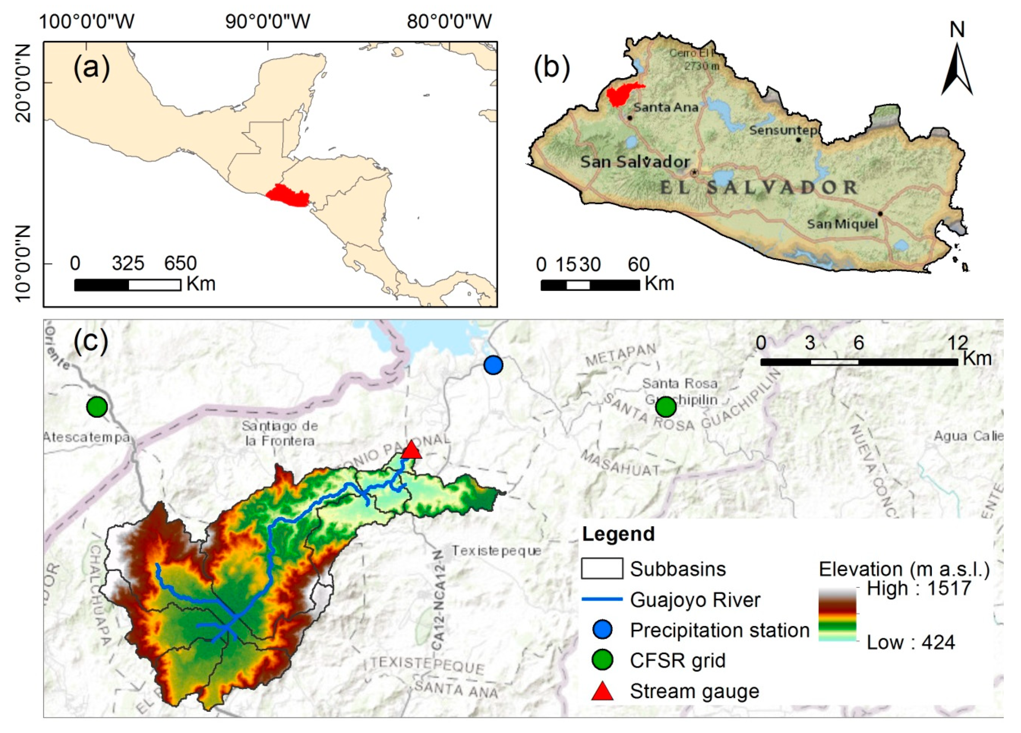
The headwaters of Guajoyo River Basin are situated in the West of El Salvador and cover about 156 km2, with terrain elevations of between 425 and 1517 m (Figure 1). The average slope in the basin is 16%, with steep slopes characterizing the highlands and relatively gentle slopes being predominant in the lowlands. The Guajoyo River is a tributary of the Lempa River, the largest and most important river in El Salvador. The studied basin, as the region in general, has a tropical climate and experiences a wet season followed by a dry season [16].
The annual historical precipitation in this area ranges from 862 to 1834 mm/year, with the average annual precipitation from 1970 to 2017 being 1373 mm/year. The wet period from May to October is clearly distinguishable, with an average rainfall of 1249 mm, equivalent to 91% of the total annual rainfall, and the dry period from November to April with a rainfall of 124 mm representing 9%. Temperature values vary mainly with elevation and show few seasonal changes, with maximum values in the months of March and April and minimum values in the months of November and December. The average annual temperature in the basin is 23 °C. The dominant soils are andosols, which are of volcanic origin, highly permeable and fertile [17,18]. The basin is covered by sixteen land use types (Table 1), being dominated by cropland, which accounts for 51% of the total area, and by pastureland (30%).
2.2. Data Sources
The SWAT model requires input of Digital Elevation Data (DEM), land use, soils, and meteorological data, such as daily precipitation, maximum and minimum temperatures, solar radiation, relative humidity and wind speed. The terrain data were obtained from the Advanced Spaceborne Thermal Emission and Reflection Radiometer (ASTER) Global Digital Elevation Model (GDEM) version 2, with a resolution of 30 × 30 m [19]. Land use maps, precipitation and streamflow data were obtained from Ministry for the Environment and Natural Resources of El Salvador (MARN). The rainfall station is located on Lake Güija at an altitude of 485 m a.s.l. The streamflow data are monthly data from 2006 to 2012 for a gauge station called Piedra–Cargada that is located at the outlet of the basin. Soil data were taken from the Harmonized World Soil Database [20]. Due to the poor quality and scarcity of measured data, other weather data (maximum, and minimum air temperatures, average wind speed, solar radiation, and relative humidity) were derived from the Climate Forecast System Reanalysis (CFSR) data set developed by the National Centers for Environmental Prediction (NCEP) in the USA [21], with a grid data of size 38 by 38 km (see Supplementary Materials, Tables S1 and S2). The CFSR data were obtained from the SWAT team at Texas A&M University (https://globalweather.tamu.edu/). Global atmospheric reanalysis such as CFSR are commonly used to provide basin–scale hydrological simulations with the required climate data, especially where measured data are scarce [22].
In this study, the software Climate Change Toolkit (CCT) (described by Vaghefi et al. [23]) had been used to prepare the data for the climate change scenarios. CCT is a platform which allows the user to extract and prepare data needed in a climate change study for application to hydrology. Data for different climate change scenarios were prepared using the CCT software. CCT database involves five sets of global 0.5° × 0.5° grid GCM data from Inter-Sectoral Impact Model Inter comparison Project (ISI-MIP5) [24]. Historical (1975–2005) and future data (2006–2099) for temperature (°C) and precipitation (mm) from five GCMs (GFDL–ESM2M, HadGEM2–ES, IPSL–CM5A–LR, MIROC, and NoerESM1–M) were downloaded (made available at http://www.2w2e.com). CCT software uses a statistical bias correction method to downscale meteorological variables from GCMs. The RCP 4.5 and 8.5 emission scenarios were used to quantify climate change on the hydrologic regime of Guajoyo River Basin.
2.3. Conceptual Model
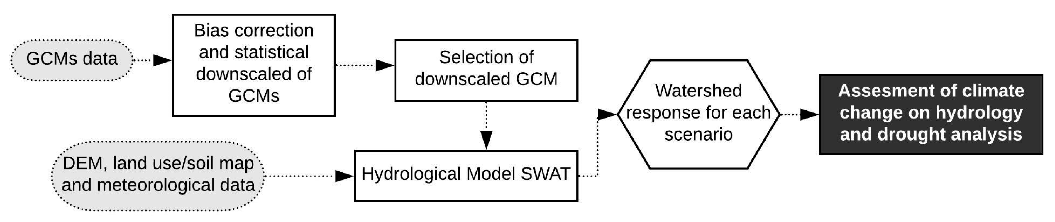
The aim of this study is to quantify the future climate and its impact on the streamflow of the Guajoyo River Basin. A SWAT model was used to develop different model setup scenarios. Under different climatic conditions in the future, specifically with respect to rainfall and temperature, the response of the basin was evaluated. The potential impact of climate change on hydrology is analyzed in two different time horizons: mid future (2040–2069), and far future (2070–2099). The 30-year period from 1975–2004 was used as a baseline. The methodology used in this study is presented in Figure 2. It includes the following steps: (1) configuration, calibration and validation of hydrological model using SWAT; (2) spatial and temporal extraction of GCMs data, bias correction and statistical downscaling of these data using CCT software; (3) analysis and comparative assessment of downscaled GCM projections according to their ability to reproduce historical climatology for the selection of GCM; (4) obtaining the results in SWAT for each scenario considered; (5) assessment of the impact of climate change in the basin by simulating the new climate conditions in the calibrated SWAT model and drought analysis.
2.4. The SWAT Hydrological Model
The hydrological modelling of Guajoyo River Basin was carried out using SWAT. The SWAT model is a semi-distributed physically based hydrological model, operating on a daily time step and used for continuous long-term simulations of a variety of processes. The major simulated hydrological variables of the SWAT model consist of surface runoff, soil and root zone infiltration, evapotranspiration, soil and snow evaporation, and return flow [25].
The SWAT model works on the principle of dividing the basin into a multiple sub-basins based on the river network and topography; subsequently, sub–basins are divided into hydrologic response units (HRUs) which have unique soil, slope and land use properties [26]. SWAT simulates the hydrological cycle based on the water balance using the following equation:
where SWt is the final soil water content (mm), SWinit is the initial soil water content (mm), t is the time in days, Rday(i) is the amount of precipitation on day i (mm), Qsurf(i) is the surface runoff (mm), Ea(i) is the evapotranspiration (mm), Wseep(i) is the percolation (mm) and Ggw(i) is the return flow (mm).
2.4.1. Model Setup
The SWAT model requires three physically based inputs to characterize a watershed: a soil map, a land cover/use map, and a DEM. The first step in SWAT model setup for a particular area are defining the watershed boundaries and analyze the drainage patterns of the terrain using a DEM of 30 m × 30 m grid size. The landuse data contains use and crop specific digital layers, suitable for use in Geographic Information System (GIS) and are one of the most important factors that control events such as runoff, evapotranspiration, sediment deposition and soil erosion [27]. The area under each landuse type and SWAT classification system are presented in Table 1. Soil maps were used to characterize each soil type from information on soil texture, hydraulic conductivity and available water content, among others, and includes one type of soil for the study area. Due to high elevation differences in the basin, four categories of slope were defined (0–5%, 5–10%, 10–20% and >20%) which cover 23, 9, 18, and 50% of the watershed, respectively. In SWAT, land use, soil and slope maps were overlaid to create the HRUs. To have a better estimation of streamflow of the basin and so as to avoid unnecessary large number of HRUs, a threshold level of 10% was established to simplify model processing and remove minor slopes, soils and land uses for each sub–basin. Finally, the Guajoyo River Basin has been divided into 11 sub-basins and 85 HRUs.
The main required climate inputs for SWAT are temperatures and precipitation, which are the ultimate climate drivers of the runoff process [28]. In this study, the SCS curve number method developed by the Soil Conservation Service [29] was used to estimate surface runoff from precipitation. The FAO Penman–Monteith method [30] was adopted to calculate the daily potential evapotranspiration. The Penman–Monteith method is recommended as the sole standard method by the United Nations Food and Agriculture Organization (FAO) and requires solar radiation, air temperature, relative humidity and wind speed [31]. Finally, once the meteorological data were loaded, the SWAT model run was started.
2.4.2. Model Calibration and Validation Procedures
The SWAT model has been calibrated and validated against observed discharge data from a gauging station using the SUFI–2 algorithm of SWAT–CUP (Calibration and Uncertainty Programs) [32]. Eleven widely used flow calibration parameters and their ranges were selected based on available literature and our previous experience, incorporating aspects of groundwater flow, runoff and soil data. To reach an acceptable calibration, three iterations (each iteration representing 500 simulations) were performed as recommended by Alemayehu et al. [33] and Pomeón et al. [34]. The parameter ranges were updated after each iteration. Among the incomplete and non-continuous measured streamflow data and considering five years as warm-up, the periods 2006–2009 and 2010–2012 were selected as the calibration and validation periods, respectively. Following the recommendations of Arnold et al. [35], the selected calibration period includes dry and wet periods to ensure that it reflects the range of conditions under which the model is expected to operate.
The model was evaluated on a monthly scale and the Nash–Sutcliffe Efficiency (NSE) was chosen as the objective function. The performance of the model for the monthly flow was evaluated according to the recommendation and performance ratings proposed by Moriasi et al. [36]. Further efficiency criteria used in this study were the R2, PBIAS, RMSE, and RSR. These statistics are defined in Table 2.
2.5. Climate Change Scenarios and Predictions
After the SWAT model was calibrated and validated under current conditions, the simulation of streamflow corresponding to future climate change were carried for future periods in two time horizons, mid future (2040–2069), and far future (2070–2099), for both RCP 4.5 and RCP 8.5 climate scenarios. Firstly, historical and future GCMs climate data was extracted from GFDL–ESM2M, HadGEM2–ES, IPSL–CM5A–LR, MIROC, and NoerESM1–M models. Second, it was necessary that GCMs products be regionalized to a specific area to obtain a meaningful interpretation of the impacts of climate change on a local scale. In addition, biases need to be corrected to eliminate existing biases in climate data [38]. In this study bias correction using statistical downscaling was used for the GCM future data, which were bias corrected against the observed data. The performance of statistical bias correction methods to downscale the meteorological variables of the GCMs is considered satisfactory in different hydro-climatological studies [39]. The observed data for the period 1975–2004 used as the base period were also corrected according to Sofaer et al. [40] (see Supplementary Materials, Tables S3 and S4). Data download, spatial downscaling and bias correction of GCMs and the observed data were carried out in the CCT software. The CCT downscaling module searches for the measured data stations and finds the one closest to the GCM grids to apply the correction factor. In this method, an additive and multiplicative correction factor has been applied to each month for temperature and precipitation, respectively.
The next step in this study was to perform a comparative analysis of GCMs products, previously downscaled and bias corrected, to select the better model according to their ability to reproduce historical climatology of the study area. The methodology used in this task is the one proposed by Pulido-Velazquez et al. [41]. This method consists of comparing means and standard deviations for a mean year on a monthly basis for historical precipitation and temperature time series and control series derived from the regionalized GCM (RCM) over the same period, in this study from 1980 to 2004. For this purpose, an indicator (Id) given by Equation (2) measures the goodness of adjustment obtained using each RCM for two statistics, mean and standard deviation, of both climatic variables:
where the subindex i is employed for a specific RCM and superscript j for the months for a mean year. V1 is the precipitation variable, V2 is the mean temperature variable, S1 the mean monthly value, S2 the monthly standard deviation for a specific RCMi.
Afterward, once the four Id indicators have been obtained for each RCM, corresponding to the mean and standard deviation of both series, the best models in terms of goodness of fit to the observed time series were selected. Finally, the simulation results from the selected RCMs such as daily precipitation, and maximum and minimum temperature data of both scenarios were used as input for the SWAT model to generate the future flows.
Trend Analysis Methods
In this study, the Mann–Kendall test for the detection of trends of annual and monthly precipitation and mean temperature, and Sen’s method for estimating of the slope of linear trends were used. Both non-parametric methods have been applied using the Microsoft Excel template application MAKESENS (Version 1.0) (more details can be found in Salmi et al. [42]). The Mann–Kendall test is one of the most widely used non–parametric tests for detecting trends in hydroclimatic series, which, contrary to parametric methods, it does not require the data to be normally distributed, requires only that it the data be independent. In addition, it has a low sensitivity to abrupt peaks due to inhomogeneous time series [43]. The presence of a statistically significant trend is evaluated using the test statistic Z. A positive value of Z indicates an upward trend and a negative value indicates a downward trend. In MAKESENS, the tested significance levels are 0.001, 0.01, 0.05 and 0.1. Details about the formulation of Mann-Kendall test can be found in Partal and Kahya [44]. The Sen’s method [45] is another very useful index that estimates the magnitude of the trend and is given for the sample of N pairs of data by:
where xj and xk are the data values at time j and k (j > k), respectively.
2.6. Drought Analysis
In this study, the standardized precipitation index (SPI) [46] and the standardized runoff index (SRI) [47] were used to characterize the meteorological and hydrological droughts, using observed precipitation and model derived runoff data for the baseline period and future simulation periods. In this study, 12-month SPI (SPI–12) and 12-month SRI (SRI–12) values were calculated using SPI Generator software developed by National Drought Mitigation Center (NDMC) [48]. A drought event is a period where SPI or SRI values are continuously negative. A drought event begins when the SPI or SRI reaches an intensity of −1.0 or less and ends when the SPI or SRI reaches a positive value. The duration of a drought event is the total number of months from the beginning to the end of the episode. The intensity of the drought event is calculated as the mean of all absolute monthly SPI or SRI values over that duration [49].
3. Results and Discussion
3.1. Performance of the SWAT Model
As discussed in the previous section, a total of 11 SWAT–parameters were optimized using the SUFI–2 algorithm of SWAT–CUP. The calibration was performed over a period of 4 years, from 2006 to 2009. The final ranges used and the final fitted values of these parameters are given in Table 3.
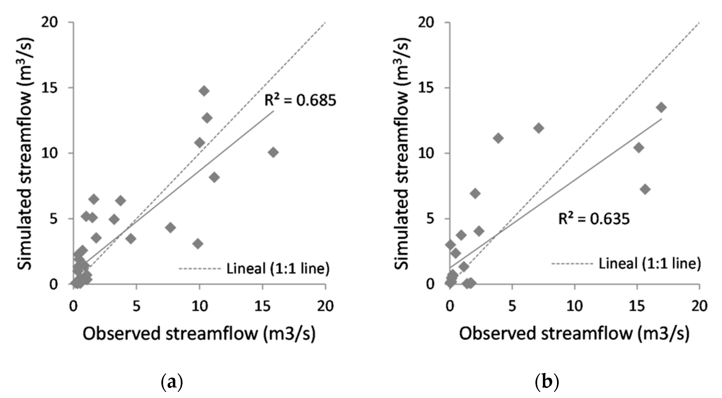
Figure 3 shows the results of the SWAT model plotted against the observed values of streamflow during model calibration and validation. As seen in the regression graphs (Figure 3), the model results showed that a systematic error of the SWAT model was the inability to simulate the peak flows. This problem seems to be common in many studies [50,51,52] and is a source of uncertainty that has been taken into account. Despite this drawback, model calibration and validation provided globally satisfactory performance statistics (Table 4), according to the criteria given by Moriasi et al. [36].
The model performance of the monthly streamflow simulation was summarized in Table 4. For the calibration period, the SWAT model simulated the streamflow reasonably well, and also proved satisfactory for the validation period. For both periods, a NSE greater than 0.5, a PBIAS less than 25% and an RSR less than 0.7, indicated a suitable calibration and validation with respect to the water balance [36]. Values of R2 greater than 0.6 also showed an acceptable model fit. These reasonable results in monthly streamflow simulation, considering the scarcity of data available in the area, allowed the SWAT model to be considered suitable for assessing hydrological responses to medium- and long-term climate change in the Guajoyo River Basin. This evaluation will be presented in the following sections. In order to demonstrate the model’s goodness-of-fit, the calibrated model was run using CHIRPS (Climate Hazards Group InfraRed Precipitation with Stations) rainfall satellite data for the period 2006–2012. The CHIRPS dataset was acquired through website (http://chg.geog.ucsb.edu/data/chirps/) and has a spatial resolution of 0.05°. With these data, good statistics were also obtained for the period 2006–2012: a NSE of 0.74, a R2 of 0.78, a PBIAS of −23.55, a RMSE of 2.29 and a RSR of 0.51.
3.2. Selection of Climate Change Models
Once the information was extracted and prepared for the study area of the five GCMs (GFDL–ESM2M, HadGEM2–ES, IPSL–CM5A–LR, MIROC, and NoerESM1–M) using CCT software, the model that best reproduced the changes for the average year for the key monthly statistics was selected. To make this selection, the Id index, defined as the sum of the absolute value of the relative difference between the statistics of the historical series and the control scenario during the 12 months of an average year, was calculated. Table 5 shows the Idi index of each RCMi on a monthly scale in the period 1980–2004. Each Idi represents the distance between the means (Δx) and the standard deviations (Δσ) of the historical and control scenarios. The models with higher Id are inferior in terms of goodness–of–fit to the observed time series. Of the five regionalized GCMs, the HadGEM2–ES model obtained a smaller Id (Id2 = 12.10) so fitted better to the historical series of precipitation and temperature. Using this validation-based approach, we are assuming that a model’s ability to simulate an observed baseline climate will be representative of the same model’s ability to project future climate. The selection of GCMs has been analyzed in a number of studies (e.g., [41,53,54]). However, there is not yet sufficient scientific consensus with respect to both the identification of unsatisfactory models, and the relation between apparently poor performance to the plausibility of future projections [55]. As discussed by Overland et al. [56], the elimination of some GCMs may narrow the range of uncertainty represented by the remaining models, but it is also true that a falsely narrow range of projections may lead to over confidence and maladaptation. In this study, and due to the big differences between the fit of this model and the others, only the HadGEM2–ES model was selected for the evaluation of the impacts of climate change.
3.3. Changes in Climate Variables under RCP Scenarios
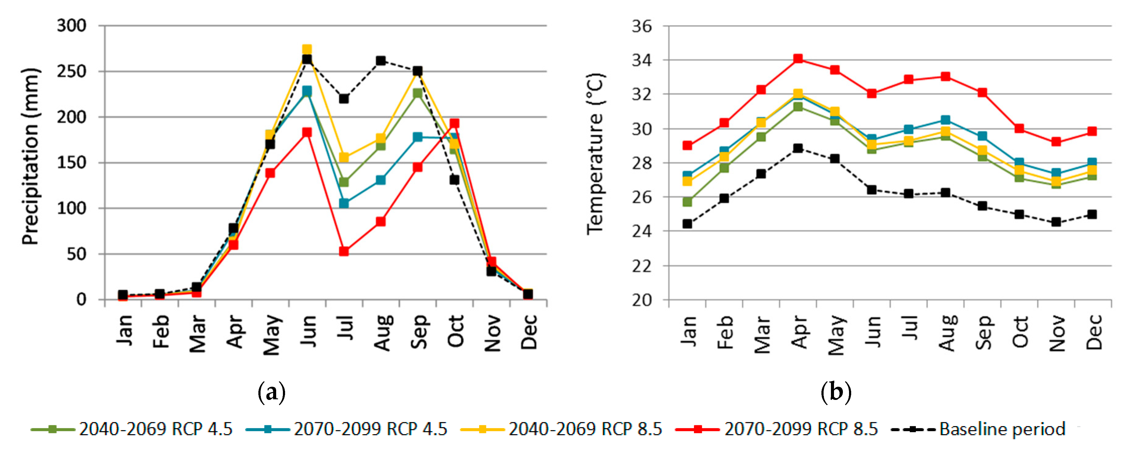
Changes in average monthly streamflows attributed to climate change, such as temperature and precipitation changes, in the mid-century and late-century periods, as compared to the baseline period for the Guajoyo River Basin for the HadGEM2–ES model, are presented in Figure 4.
Figure 4a shows the bimodal distribution of precipitation of the rainy summer season for the baseline and future periods, with the maximum values in the months of June and September–October and the relative minimums in July and August. This relative minimum is known as the “Mid–Summer Drought” (MSD) [57] which is considered one of the most important regional climate variability modulators [58]. On a monthly scale, considering the dry season, precipitation is expected to increase in both scenarios and in both future periods for November and December. Specifically, for the regionalized HadGEM2–ES model, precipitation will increase by around 20% in November. However, during the rainy season (between May and October), the changes obtained show decreases in precipitation, except in October, when precipitation is expected to increase by around 27% in the medium term and 41% by the end of the century. The results show that the decrease in precipitation during the months of the wet season could occur with greater intensity in the months of July and August, with reductions of about 35% in the medium term and 61% in the long term, producing an intensification of the MSD. On the other hand, Figure 4b shows the results for the average temperature. The greatest increases in mean temperature were obtained during the summer months (July, August and September), with average increases of 3.1 °C (RCP 4.5) and 3.3 °C (RCP 8.5) by mid-century and 4 °C (RCP4.5) and 6.7 °C (RCP 8.5) by the end of the century. Similar trends of these climatic variables in El Salvador were found in the work carried out by the MARN (2017) [58].
Table 6 summarizes average annual climate variables for the baseline as well as under both emissions scenarios and both future periods of the HadGEM2–ES model. On an annual scale, the results show that precipitation will follow a decreasing trend under future conditions, whilst average temperatures will follow an increasing trend. Overall, the maximum decrease in precipitation of up to 36% is expected under RCP 8.5 in late century compared to the baseline precipitation of 1435.60 mm/year, in accord with the study of CEPAL (2010) [59], in which it was predicted that rainfall in El Salvador will decrease between 27% and 32%. In addition, the highest average temperatures are expected at the end of the century, with temperatures 12% and 21% higher than the base temperature of 26.12 °C for RCP 4.5 and 8.5 respectively. The results obtained are consistent with the findings of Conde–Álvarez and Saldaña–Zorrilla [60], which indicated that warming in Latin America by the end of the century, according to different models, will be from 1 to 6 °C for different emission scenarios.
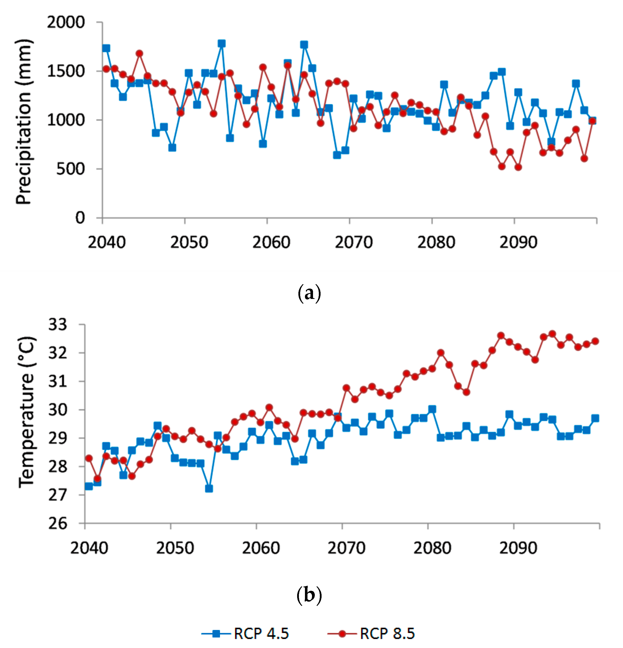
Figure 5 shows the average yearly precipitation and temperature in the basin from 2040 to 2099. Figure 5a shows how the future trend of precipitation is decreasing. In the medium term, the predicted decrease is greater in the RCP 4.5. However, in the long term, the predicted decrease in precipitation is higher for RCP 8.5, as shown in Table 6. Future temperature trends (Figure 5b) show that Guajoyo River Basin will likely experience warmer conditions in the future, the largest increase being for the RCP 8.5 scenario.
Trends in the Climatic Variables
The results of the Mann-Kendall and Sen’s slope analysis of precipitation and mean temperature for the period 2040–2099 are provided in Table 7. As shown, the majority of the trends in the monthly precipitation series were downward, with a significant decrease in the summer months. In the case of monthly temperatures, the majority of months showed significant upward trends in both scenarios.
The trend analysis showed a decrease in annual precipitation of 3.70 mm/year with a significance level of 0.1 and 13.17 mm/year with a significance level of 0.001 for RCP 4.5 and RCP 8.5 scenarios, respectively. The annual mean temperature indicated a significant upward trend (0.001 level of significance). The temperature increased 0.02 °C/year for the RCP 4.5 scenario and 0.08 °C/year for the RCP 8.5 scenario.
3.4. Changes in Water Balance under RCP Scenarios
The impact of climate change on water availability was assessed according to the climate change scenarios for the basin. In this study, it was assumed that future land use change was constant in order to investigate the impact with respect to change in climate variables, keeping all other factors constant. After the SWAT hydrological model was calibrated and validated, the downscaled future precipitation and temperature predictions of the HadGEM2–ES model under two emission scenarios were used as input to explore streamflow responses to projected future climate change scenarios. Table 8 summarizes the response of basin’s water balance components (precipitation, evapotranspiration, total water yield and groundwater recharge) under two RCP scenarios in terms of average annual values and percentage change from the baseline condition.
It was apparent from this table that with an increase in temperature and a decrease in precipitation, there will be an increasing trend in the ET and in the ET/P ratio but a decreasing trend in the WYLD and DA_RCHG. ET will increase in both future scenarios. As a consequence of climate warming, the midcentury ratio of ET/P could be between 0.47 and 0.50, and at the end of century could be between 0.54 and 0.60. The annual water yield for the basin for baseline period was 720.72 mm. The WYLD for midcentury is likely to decrease under the projected climate scenarios and it could vary between 450.33 mm and 522.18 mm. Also, a considerable reduction in recharges to deep aquifers is also predicted. On the other hand, end-of-century water yield can be predicted as a drastic decrease of approximately 50% (359.47 mm) and 63% (268.87 mm) for the RCP 4.5 and RCP 8.5 scenarios. The results obtained in this study were in accord with previous researches such as the study of CEPAL (2010) [59], in which it was predicted that the total availability of renewable water could decrease between 35% and 63% by the end of the century, with El Salvador being one of the most affected countries. Maurer et al. [9] projected an increase of the average temperature and a reduction of average precipitation that imply a reduction, on average by 13 to 24%, in inflows to major reservoirs of the Lempa River Basin for end of the 21st century. Also, a decreasing runoff across all Central America, even in areas where precipitation increases, was obtained in the work of Imbach et al. [10].
3.5. Future Projections of Drought
The SPI–12 and SRI–12 values are given in Table 9 and were calculated to quantify the effects of observed changes under historical climate variability and projected future climate change on meteorological and hydrological drought.
The number of meteorological and hydrological drought events was 9 and 5, with an average duration of 12 and 14 months, and an average intensity of 1.60 and 1.95 respectively for the baseline period. The mid-century RCP 4.5 scenario indicated that the number of meteorological and hydrological drought events will be fewer but will be of greater duration and intensity. For this scenario, the number of drought events will increase for both types of drought in the long term, but with less intensity than for the baseline period. In the case of meteorological droughts, drought events will be longer. In RCP 8.5 scenario, the number of drought events was lower, but with an increase of duration in both meteorological and hydrological droughts, and the intensity only in the meteorological type. This is consistent with the study of Esquivel et al. [61] which indicates that future droughts will be more pronounced than current droughts, both in terms of the amount of resources available and the duration of events. Also, the IPCC-AR5 (2014) [62] reported that long-term changes in rainfall in Latin America will cause longer periods of drought.
4. Conclusions
The Guajoyo River Basin is located in an area of environmental interest in terms of international protection figures which guarantees water supply for local communities, as well as being important in regional development through agro-tourism and coffee activities. In the present study, the impacts of a climate change on meteorological variables (i.e., precipitation and temperature) have been analyzed, as well as on the main hydrological variables (i.e., ET, WYLD and DA_RCHG) and on the droughts of the Guajoyo River Basin. The future projections of precipitation and temperature of five GCMs (GFDL–ESM2M, HadGEM2–ES, IPSL–CM5A–LR, MIROC, and NoerESM1–M) were considered. After the analysis and comparative evaluation of these projections, the best model was selected according to its ability to reproduce the historical climate. The physically based semi-distributed SWAT model was employed to quantify the impacts of future climate variations on the hydrological processes driven by a regionalized HadGEM2–ES for RCP 4.5 and RCP 8.5 climate scenarios. SWAT acceptably simulated monthly streamflow despite data scarcity, and the results in the basin for the historic baseline were compared with future periods (2040–2069 and 2070–2099).
The results of this analysis indicated an annual decrease in precipitation of 15% (RCP 4.5) and 7% (RCP 8.5) during mid-century and 21% (RCP 4.5) and 36% (RCP 8.5) during the end of the century with respect to the base period (1975–2004). The annual mean temperature showed an increase for the midcentury period of 9% and 11% and an increase of 12% and 21% for the late century period, under RCP 4.5 and RCP 8.5 scenarios, respectively. The Mann–Kendall analysis indicated for the future period (2040–2099) a significant downward trend in annual precipitation and a significant upward trend in annual mean temperatures for both emission scenarios. For the hydrological cycle, the results suggested that the impact of climate change will be negative in the medium and long term. The availability of water will experience a decrease. As for WYLD, a decrease of 37% (RCP 4.5) and 27% (RCP 8.5) was obtained for the medium term and 50% (RCP 4.5) and 63% (RCP 8.5) for the end of the century. Similarly, a reduction of aquifer recharge was predicted by 43% and 33% for the middle of the century and by 55% and 71% at the end of the century, under RCP 4.5 and RCP 8.5 respectively. The ET/P ratio showed an increasing trend, going from 0.36 in the base period to 0.54 (RCP 4.5) and 0.6 (RCP 8.5) in the long term. Additionally, the impact of climate change on droughts has been analyzed using two drought indexes, SPI and SRI. In both studied scenarios it was obtained that in the future the droughts will be more pronounced than current droughts, being more intense and of longer duration.
This study supports and raises awareness of the possible future impacts of climate change on the water balance and on the droughts of this river basin. The results show that the availability of water will be significantly affected in the medium and long term, and therefore, policies must be developed to adapt to climate change to ensure environmental and economic sustainability of this area.
Supplementary Materials
The following are available online at https://www.mdpi.com/2073-4441/11/11/2360/s1, Table S1: Climatic stations used in the basin, Table S2: Monthly data used for model calibration and validation (2001–2012), Table S3: Modelled past data. Annual data for baseline period (1975–2004), Table S4: Modelled future data. Annual data for future period 2040–2099.
Author Contributions
All authors contributed significantly to the development of the methodology applied in this study. P.B.-G. and P.J.-S. designed the experiments and wrote the article. J.S.-A. provided technical assistance and reviewed and helped to prepare this paper for publication. J.P.-S. provided many important advices on the concept of methodology and reviewed this manuscript.
Funding
This research received no external funding.
Acknowledgments
We thank the Ministry for the Environment and Natural Resources (MARN) of El Salvador for their available data. We also would like to thank Jethro David Howard for proof-reading the text.
Conflicts of Interest
The authors declare no conflict of interest.
References
- Verma, S.; Bhattarai, R.; Bosch, N.S.; Cooke, R.C.; Kalita, P.K.; Markus, M. Climate change impacts on flow, sediment and nutrient export in a Great Lakes watershed using SWAT. Clean Soil Air Water 2015, 43, 1464–1474. [Google Scholar] [CrossRef]
- Zhang, Y.; You, Q.; Chen, C.; Ge, J. Impacts of climate change on streamflows under RCP scenarios: A case study in Xin River Basin, China. Atmos. Res. 2016, 178, 521–534. [Google Scholar] [CrossRef]
- Chattopadhyay, S.; Jha, M.K. Hydrological response due to projected climate variability in Haw River watershed, North Carolina, USA. Hydrol. Sci. J. 2016, 61, 495–506. [Google Scholar] [CrossRef]
- Bhatta, B.; Shrestha, S.; Shrestha, P.K.; Talchabhadel, R. Evaluation and application of a SWAT model to assess the climate change impact on the hydrology of the Himalayan River Basin. Catena 2019, 181, 104082. [Google Scholar] [CrossRef]
- Parry, M.L.; Canziani, O.F.; Palutikof, J.P.; Van der Linden, P.J.; Hanson, C.E. IPCC, 2007. Climate Change 2007: Impacts, Adaptation and Vulnerability. Contribution of Working Group II to the Fourth Assessment Report of the Intergovernmental Panel on Climate Change; Cambridge University Press: Cambridge, UK, 2007; p. 976. [Google Scholar]
- Fischer, G.; Shah, M.; Tubiello, F.N.; Van Velhuizen, H. Socio–economic and climate change impacts on agriculture: An integrated assessment, 1990–2080. Philos. T. Roy. Soc. B 2005, 360, 2067–2083. [Google Scholar] [CrossRef] [PubMed]
- Tubiello, F.N.; Rosenzweig, C. Developing climate change impact metrics for agriculture. Integrat. Assess. 2008, 8, 165–184. [Google Scholar]
- Campos, M.; Herrador, D.; Manuel, C.; McCall, M.K. Estrategias de adaptación al cambio climático en dos comunidades rurales de México y El Salvador. BAGE 2013, 61, 329–349. [Google Scholar]
- Maurer, E.P.; Adam, J.C.; Wood, A.W. Climate model based consensus on the hydrologic impacts of climate change to the Rio Lempa basin of Central America. Hydrol. Earth Syst. Sci. 2009, 13, 183–194. [Google Scholar] [CrossRef] [Green Version]
- Imbach, P.; Molina, L.; Locatelli, B.; Roupsard, O.; Mahé, G.; Neilson, R.; Corrales, L.; Scholze, M.; Ciais, P. Modeling potential equilibrium states of vegetation and terrestrial water cycle of mesoamerica under climate change scenarios. J. Hydrometeorol. 2012, 13, 665–680. [Google Scholar] [CrossRef]
- Aguilar, M.Y.; Pacheco, T.R.; Tobar, J.M.; Quiñónez, J.C. Vulnerability and adaptation to climate change of rural inhabitants in the central coastal plain of El Salvador. Clim. Res. 2009, 40, 187–198. [Google Scholar] [CrossRef] [Green Version]
- Parajuli, P.B. Assessing sensitivity of hydrologic responses to climate change from forested watershed in Mississippi. Hydrol. Process. 2010, 24, 3785–3797. [Google Scholar] [CrossRef]
- Zhang, X.; Xu, Y.; Hao, F.; Li, C.; Wang, X. Hydrological components variability under the impact of climate change in a semi–arid river basin. Water 2019, 11, 1122. [Google Scholar] [CrossRef]
- Ji, L.; Duan, K. What is the main driving force of hydrological cycle variations in the semiarid and semi–humid Weihe River Basin, China? Sci. Total Environ. 2019, 684, 254–264. [Google Scholar] [CrossRef] [PubMed]
- Senent–Aparicio, J.; Pérez–Sánchez, J.; Carrillo–García, J.; Soto, J. Using SWAT and fuzzy TOPSIS to assess the impact of climate change in the headwaters of the segura river Basin (SE Spain). Water 2017, 9, 149. [Google Scholar] [CrossRef]
- MARN. Plan Nacional de Gestión Integrada del Recurso Hídrico de El Salvador, con Énfasis en Zonas Prioritarias, 1st ed.; Ministerio de Medio Ambiente y Recursos Naturales: San Salvador, El Salvador, 2017. Available online: http://www.marn.gob.sv/plan-nacional-de-gestion-integrada-del-recurso-hidrico/ (accessed on 1 May 2019).
- Wada, K. The distinctive properties of Andosols. In Advances in Soil Science; Springer: New York, NY, USA, 1985; pp. 173–229. [Google Scholar] [CrossRef]
- Levard, C.; Basile–Doelsch, I. Geology and mineralogy of imogolite–type materials. In Nanosized Tubular Clay Minerals; Elsevier: Amsterdam, The Netherlands, 2016; pp. 49–65. [Google Scholar] [CrossRef]
- ASTER Global Digital Elevation Map. Available online: https://asterweb.jpl.nasa.gov/gdem.asp (accessed on 20 May 2019).
- Fischer, G.; Nachtergaele, F.; Prieler, S.; Velthuizenvan, H.; Verelst, L.; Wiberg, D. Global Agro–Ecological Zones Assessment for Agriculture (GAEZ 2008); IIASA: Laxenburg, Austria; FAO: Rome, Italy, 2008. [Google Scholar]
- Saha, S.; Moorthi, S.; Pan, H.L.; Wu, X.; Wang, J.; Nadiga, S.; Tripp, P.; Kistler, R.; Woollen, J.; Behringer, D.; et al. The NCEP climate forecast system reanalysis. B. Am. Meteorol. Soc. 2010, 91, 1015–1057. [Google Scholar] [CrossRef]
- Tarawneh, E.; Bridge, J.; Macdonald, N. A pre–calibration approach to select optimum inputs for hydrological models in data–scarce regions. Hydrol. Earth Syst. Sci. 2016, 70, 4391–4407. [Google Scholar] [CrossRef]
- Vaghefi, S.A.; Abbaspour, N.; Kamali, B.; Abbaspour, K.C. A toolkit for climate change analysis and pattern recognition for extreme weather conditions—Case study: California–Baja California peninsula. Environ. Model. Softw. 2017, 96, 181–198. [Google Scholar] [CrossRef]
- Hempel, S.; Frieler, K.; Warszawski, L.; Schewe, J.; Piontek, F. A trend-preserving bias correction—The isi-mip approach. Earth Syst. Dynam. 2013, 4, 219–236. [Google Scholar] [CrossRef]
- Arnold, J.G.; Srinivasan, R.; Muttiah, R.S.; Williams, J.R. Large area hydrologic modeling and assessment Part I: Model development. J. Am. Water Resour. Assoc. 1998, 34, 73–89. [Google Scholar] [CrossRef]
- Arnold, J.G.; Kiniry, J.R.; Srinivasan, R.; Williams, J.R.; Haney, E.B.; Neitsch, S.L. Soil & Water Assessment Tool—Input/Output Documentation; Version 2012; Texas Water Resources Institute: College Station, TX, USA, 2012; p. 650. Available online: https://swat.tamu.edu/docs/ (accessed on 20 May 2019).
- Singh, V.; Bankar, N.; Salunkhe, S.S.; Bera, A.K.; Sharma, J.R. Hydrological stream flow modelling on Tungabhadra catchment: Parameterization and uncertainty analysis using SWAT CUP. Curr. Sci. India 2013, 104, 1187–1199. [Google Scholar]
- Emami, F.; Koch, M. Modeling the impact of climate change on water availability in the Zarrine River Basin and inflow to the Boukan Dam, Iran. Climate 2019, 7, 51. [Google Scholar] [CrossRef]
- USDA, SCS. Hydrology. In National Engineering Handbook, Section 4; USDA Soil Conservation Service: Washington, DC, USA, 1972. [Google Scholar]
- Monteith, J.L. Evaporation and environment. Symp. Soc. Exp. Biol. 1965, 19, 205–234. [Google Scholar] [PubMed]
- Allen, R.G.; Pereira, L.S.; Raes, D.; Smith, M. Crop Evapotranspiration: Guidelines for Computing Crop Water Requirements; Food and Agriculture Organization of the United Nations: Rome, Italy, 1998. [Google Scholar]
- Abbaspour, K.C.; Vejdani, M.; Haghighat, S. SWAT–CUP calibration and uncertainty programs for SWAT. In Proceedings of the Modsim 2007: International Congress on Modelling and Simulation, Christchurch, New Zealand, 3–8 December 2007; pp. 1603–1609. [Google Scholar]
- Alemayehu, T.; van Griensven, A.; Bauwens, W. Evaluating CFSR and WATCH data as input to swat for the estimation of the potential evapotranspiration in a data–scarce Eastern–African catchment. J. Hydrol. Eng. 2016, 21, 16. [Google Scholar] [CrossRef]
- Poméon, T.; Diekkrüger, B.; Springer, A.; Kusche, J.; Eicker, A. Multi–objective validation of SWAT for sparsely–gauged West African River basins—A remote sensing approach. Water 2018, 10, 451. [Google Scholar] [CrossRef]
- Arnold, J.G.; Moriasi, D.; Gassman, P.W.; Abbaspour, K.C.; White, M.J.; Srinivasan, R.; Santhi, C.; Harmel, R.D.; van Griensven, A.; Van Liew, M.W.; et al. SWAT: Model use, calibration, and validation. Trans. ASABE 2012, 55, 1491–1508. [Google Scholar] [CrossRef]
- Moriasi, D.N.; Arnold, J.G.; van Liew, M.W.; Bingner, R.L.; Harmel, R.D.; Veith, T.L. Model evaluation guidelines for systematic quantification of accuracy in watershed simulations. Trans. ASABE 2007, 50, 885–900. [Google Scholar] [CrossRef]
- Gupta, H.V.; Kling, H.; Yilmaz, K.K.; Martinez, G.F. Decomposition of the mean squared error and NSE performance criteria: Implications for improving hydrological modelling. J. Hydrol. 2009, 377, 80–91. [Google Scholar] [CrossRef] [Green Version]
- Chen, J.; Brissette, F.P.; Chaumont, D.; Braun, M. Performance and uncertainty evaluation of empirical downscaling methods in quantifying the climate change impacts on hydrology over two North American river basins. J. Hydrol. 2013, 479, 200–214. [Google Scholar] [CrossRef]
- Vaghefi, S.A.; Iravani, M.; Sauchyn, D.; Andreichuk, Y.; Goss, G.; Faramarzi, M. Regionalization and parameterization of a hydrologic model significantly affect the cascade of uncertainty in climate–impact projections. Clim. Dyn. 2019, 53, 2861–2886. [Google Scholar] [CrossRef]
- Sofaer, H.R.; Barsugli, J.J.; Jarnevich, C.S.; Abatzoglou, J.T.; Talbert, M.K.; Miller, B.W.; Morisette, J.T. Designing ecological climate change impact assessments to reflect key climatic drivers. Glob. Change Biol. 2017, 23, 2537–2553. [Google Scholar] [CrossRef] [PubMed]
- Pulido–Velazquez, D.; García–Aróstegui, J.L.; Molina, J.L.; Pulido–Velazquez, M. Assessment of future groundwater recharge in semi–arid regions under climate change scenarios (Serral–Salinas aquifer, SE Spain). Could increased rainfall variability increase the recharge rate? Hydrol. Process. 2015, 29, 828–844. [Google Scholar] [CrossRef]
- Salmi, T.; Maatta, A.; Anttila, P.; Airola, T.R.; Amnell, T. Detecting Trends of Annual Values of Atmospheric Pollutants by the Mann–Kendal Test and Sen’s Slope Estimates—The Excel Template Application MAKESENS; User Manual; Air Quality, Finish Meteorological Institute: Helsinki, Finland, 2002; p. 35. [Google Scholar]
- Senent-Aparicio, J.; Liu, S.; Pérez-Sánchez, J.; López-Ballesteros, A.; Jimeno-Sáez, P. Assessing impacts of climate variability and reforestation activities on water resources in the headwaters of the Segura River Basin (SE Spain). Sustainability 2018, 10, 3277. [Google Scholar] [CrossRef] [Green Version]
- Partal, T.; Kahya, E. Trend analysis in Turkish precipitation data. Hydrol. Process. 2006, 20, 2011–2026. [Google Scholar] [CrossRef]
- Sen, P.K. Estimates of the regression coefficient based on Kendall’s tau. J. Am. Stat. Assoc. 1968, 63, 1379–1389. [Google Scholar] [CrossRef]
- McKee, T.B.; Doesken, N.J.; Kleist, J. The relationship of drought frequency and duration to time scales. In Proceedings of the 8th Conference on Applied Climatology, Anaheim, CA, USA, 17–22 January 1993; pp. 179–184. [Google Scholar]
- Shukla, S.; Wood, A.W. Use of a standardized runoff index for characterizing hydrologic drought. Geophys. Res. Lett. 2008, 35, L02405. [Google Scholar] [CrossRef] [Green Version]
- NDMC. SPI Generator Software. University of Nebraska–Lincoln, USA. 2019. Available online: https://drought.unl.edu/droughtmonitoring/SPI/SPIProgram.aspx (accessed on 23 July 2019).
- WMO. Standardized Precipitation Index User Guide; WMO–No. 1090; WMO: Geveva, Switzerland, 2012; Available online: https://library.wmo.int/doc_num.php?explnum_id=7768 (accessed on 23 July 2019).
- Jimeno–Sáez, P.; Senent–Aparicio, J.; Pérez–Sánchez, J.; Pulido–Velazquez, D. A Comparison of SWAT and ANN models for daily runoff simulation in different climatic zones of Peninsular Spain. Water 2018, 10, 192. [Google Scholar] [CrossRef] [Green Version]
- Spellman, P.; Webster, V.; Watkins, D. Bias correcting instantaneous peak flows generated using a continuous, semi–distributed hydrologic model. J. Flood Risk Manag. 2018, 11, e12342. [Google Scholar] [CrossRef] [Green Version]
- Čerkasova, N.; Umgiesser, G.; Ertürk, A. Assessing climate change impacts on streamflow, sediment and nutrient loadings of the Minija River (Lithuania): A hillslope watershed discretization application with high–resolution spatial inputs. Water 2019, 11, 676. [Google Scholar] [CrossRef] [Green Version]
- McSweeney, C.F.; Jones, R.G.; Lee, R.W.; Rowell, D.P. Selecting CMIP5 GCMs for downscaling over multiple regions. Clim. Dyn. 2015, 44, 3237–3260. [Google Scholar] [CrossRef] [Green Version]
- Ahmed, K.; Sachindra, D.A.; Shahid, S.; Demirel, M.C.; Chung, E.S. Selection of multi-model ensemble of GCMs for the simulation of precipitation based on spatial assessment metrics. Hydrol. Earth Syst. Sci. 2019. Discuss, in review. [Google Scholar] [CrossRef] [Green Version]
- Knutti, R.; Furrer, R.; Tebaldi, C.; Cermak, J.; Meehl, G.A. Challenges in combining projections from multiple climate models. J. Clim. 2010, 23, 2739–2758. [Google Scholar] [CrossRef] [Green Version]
- Overland, J.E.; Wang, M.; Bond, N.A.; Walsh, J.E.; Kattsov, V.M.; Chapman, W.L. Considerations in the selection of global climate models for regional climate projections: The Arctic as a case study. J. Clim. 2011, 24, 1583–1597. [Google Scholar] [CrossRef]
- Magaña, V.; Amador, J.A.; Medina, S. The midsummer drought over Mexico and Central America. J. Clim. 1999, 12, 1577–1588. [Google Scholar] [CrossRef]
- MARN. Modelos de Simulación y Escenarios Climáticos para El Salvador (Nacional, Regional y Local); Ministerio de Medio Ambiente y Recursos Naturales, Centro del Agua del Trópico Húmedo para América Latina y el Caribe: San Salvador, El Salvador, 2017. Available online: http://rcc.marn.gob.sv/xmlui/handle/123456789/347 (accessed on 15 August 2019).
- CEPAL. La Economía del Cambio Climático en Centroamérica—Síntesis 2010; Comisión Económica para América Latina y El Caribe (CEPAL): Naciones Unidas, México, 2010. [Google Scholar]
- Conde–Álvarez, C.; Saldaña–Zorrilla, O. Cambio climático en América Latina y el Caribe: Impactos, vulnerabilidad y adaptación. Revista Ambiente y Desarrollo 2007, 23, 23–30. [Google Scholar]
- Esquivel, M.; Grünwaldt, A.; Paredes, J.R.; Rodríguez–Flores, E. Vulnerabilidad al Cambio Climático de los Sistemas de Producción Hidroeléctrica en Centroamérica y sus Opciones de Adaptación, Resumen Ejecutivo; Sector de Cambio Climático y Sector de Energía, Banco Interamericano de Desarrollo (BID): Madrid, Spain, 2016; Available online: http://expertosenred.olade.org/wp-content/uploads/sites/8/2017/01/Vulnerabilidad-al-cambio-climatico-de-los-sistemas-de-produccion-hidroelectrica-en-Centroamerica-y-sus-opciones-de-adaptacion-1.pdf (accessed on 23 August 2019).
- IPCC–AR5. Climate change 2013, The Physical Science Basis, Working Group I Contribution to the Fifth Assessment Report of the Intergovernmental Panel on Climate Change; Cambridge University Press: Cambridge, UK, 2014; ISBN 978-1-107-66182-0. [Google Scholar]
Figure 1.
Location map: (a) Location of El Salvador in Central America; (b) Location of the Guajoyo River Basin in El Salvador; (c) Subbasins, Digital Elevation Data (DEM), river and hydro-meteorological stations of Guajoyo River Basin.
Figure 1.
Location map: (a) Location of El Salvador in Central America; (b) Location of the Guajoyo River Basin in El Salvador; (c) Subbasins, Digital Elevation Data (DEM), river and hydro-meteorological stations of Guajoyo River Basin.

Figure 2.
Flowchart for the methodology adopted in the present study.

Figure 3.
Regression plots of observed versus simulated monthly streamflows for the (a) calibration period (2006–2009), and (b) validation period (2010–2012).
Figure 3.
Regression plots of observed versus simulated monthly streamflows for the (a) calibration period (2006–2009), and (b) validation period (2010–2012).

Figure 4.
Comparison of monthly mean (a) precipitation and (b) temperature between baseline period (1975–2004) and mid and far future under RCP 4.5 and 8.5 for the HadGEM2–ES model.
Figure 4.
Comparison of monthly mean (a) precipitation and (b) temperature between baseline period (1975–2004) and mid and far future under RCP 4.5 and 8.5 for the HadGEM2–ES model.

Figure 5.
Temporal variations of the projected climatic variables under RCP 4.5 and 8.5: (a) precipitation for 2040–2099 and (b) temperature for 2040–2099.
Figure 5.
Temporal variations of the projected climatic variables under RCP 4.5 and 8.5: (a) precipitation for 2040–2099 and (b) temperature for 2040–2099.


Table 1.
Land use type of the Guajoyo River Basin.
| Land Use Type | Area (km2) | % Coverage |
|---|---|---|
| Commercial | 0.66 | 0.42 |
| Sugarcane | 0.68 | 0.43 |
| Range–Grasses | 0.97 | 0.62 |
| Residential–High Density | 1.70 | 1.09 |
| Forest–Deciduous | 2.00 | 1.28 |
| Forest–Mixed | 2.35 | 1.50 |
| Southwestern US (Arid) Range | 3.22 | 2.06 |
| Meadow Bromegrass | 3.22 | 2.06 |
| Forest–Evergreen | 3.84 | 2.46 |
| Residential–Medium Density | 4.27 | 2.74 |
| Coffee | 5.75 | 3.69 |
| Shrubland | 11.51 | 7.38 |
| Pasture | 12.47 | 7.99 |
| Range–Grasses | 31.44 | 20.15 |
| Dryland cropland and pasture | 34.44 | 22.07 |
| Agricultural Land–Generic | 37.52 | 24.05 |
| Performance Metric | Equation | Range |
|---|---|---|
| Nash–Sutcliffe efficiency coefficient (NSE) | [−∞, 1] | |
| Coefficient of determination (R2) | [0, 1] | |
| Percent bias (PBIAS) | [−∞, ∞] | |
| Root mean squared error (RMSE) | [0, ∞] | |
| RMSE–observations standard deviation ratio (RSR) | [0, ∞] |
Oi is the i-th observed data, is the mean of the observed data, Si is the i-th simulated data, is the mean of the simulated data and n is the total number of observations.
Table 3.
Calibration of SWAT parameters for the Guajoyo River Basin.
| Parameter 1 | Description | Final Range Used in Calibration | Fitted Value | Final Value |
|---|---|---|---|---|
| r_CN2.mgt | SCS runoff curve number | −0.2 to 0.2 | −0.09 | [63.40–75.17] 2 |
| v_ALPHA_BF.gw | Baseflow alpha factor (days−1) | 0 to 0.65 | 0.09 | 0.09 |
| a_GW_DELAY.gw | Groundwater delay time (days) | −10 to 60 | −2.90 | 28.07 |
| a_GWQMN.gw | Threshold depth of water in the shallow aquifer for return flow to occur (mm) | 200 to 1500 | 1407.70 | 2407.70 |
| v_GW_REVAP.gw | Groundwater revap coefficient | 0.02 to 0.15 | 0.13 | 0.13 |
| a_RCHRG_DP.gw | Deep aquifer percolation fraction | −0.02 to 0.03 | 0.02 | 0.07 |
| a_REVAPMN.gw | Threshold depth of water in the shallow aquifer for revap or percolation to the deep aquifer to occur (mm) | −150 to 150 | −85.50 | 664.5 |
| v_CANMX.hru | Maximum canopy storage (mm) | 1 to 10 | 4.47 | 4.47 |
| v_EPCO.bsn | Plant uptake compensation factor | 0.5 to 1 | 0.87 | 0.87 |
| v_ESCO.bsn | Soil evaporation compensation factor | 0.3 to 0.9 | 0.79 | 0.79 |
| r_SOL_AWC.sol | Available water capacity of the soil layer (mm H2O/mm soil) | −0.02 to 0.02 | −0.01 | [0.06–0.10] 3 |
1 The qualifier (r_) refers to relative change, i.e., the current parameter must be multiplied by (1 + the value obtained in calibration), (v_) means that the value of the existing parameter must be replaced by the value obtained in calibration, and (a_) refers to absolute change, i.e., the fitted value must be added to the existing value of the parameter. 2 Varies by HRU. 3 Varies by soil layer.
Table 4.
SWAT model performance of calibration and validation.
| Performance Metric | Calibration | Validation |
|---|---|---|
| NSE | 0.67 | 0.63 |
| R2 | 0.69 | 0.64 |
| PBIAS (%) | −9.04 | −8.80 |
| RMSE (m3/s) | 2.35 | 3.12 |
| RSR | 0.58 | 0.61 |
Table 5.
Id index of each RCM.
| RCMs | Monthly Series | |||||
|---|---|---|---|---|---|---|
| Precipitation | Temperature | Id | ||||
| Id (Δx) | Id (Δσ) | Id (Δx) | Id (Δσ) | |||
| 1 | GFDL–ESM2M | 2.14 | 11.18 | 1.22 | 3.76 | 18.30 |
| 2 | HadGEM2–ES | 1.78 | 5.95 | 1.63 | 2.74 | 12.10 |
| 3 | IPSL–CM5A–LR | 1.51 | 10.93 | 1.23 | 4.15 | 17.82 |
| 4 | MIROC | 2.65 | 9.30 | 1.21 | 9.17 | 22.33 |
| 5 | NoerESM1–M | 1.52 | 8.13 | 1.23 | 5.45 | 16.33 |
Table 6.
Average climate variables changes.
| Model | Scenario | Time Period | Precipitation (mm) | Temperature (°C) | ||
|---|---|---|---|---|---|---|
| Value | Change with Respect to Baseline | Value | Change with Respect to Baseline | |||
| Baseline | 1975–2004 | 1435.60 | – | 26.12 | – | |
| HadGEM2–ES | RCP 4.5 | 2040–2069 | 1219.12 | −216.48 (−15%) | 28.45 | +2.33 (+9%) |
| 2070–2099 | 1129.62 | −305.98 (−21%) | 29.30 | +3.19 (+12%) | ||
| RCP 8.5 | 2040–2069 | 1332.64 | −102.96 (−7%) | 28.95 | +2.84 (+11%) | |
| 2070–2099 | 919.07 | −516.53 (−36%) | 31.49 | +5.38 (+21%) | ||
Table 7.
Trend analysis results for monthly and annual precipitation and mean temperature.
| Month | Precipitation RCP 4.5 | Temperature RCP 4.5 | Precipitation RCP 8.5 | Temperature RCP 8.5 | ||||||||
|---|---|---|---|---|---|---|---|---|---|---|---|---|
| Test Z | Sig. | Qi | Test Z | Sig. | Qi | Test Z | Sig. | Qi | Test Z | Sig. | Qi | |
| January | −0.49 | −0.01 | 3.78 | *** | 0.03 | 0.16 | 0.00 | 7.79 | *** | 0.07 | ||
| February | 0.10 | 0.00 | 4.98 | *** | 0.03 | −0.56 | −0.01 | 7.57 | *** | 0.07 | ||
| March | −0.17 | −0.01 | 4.02 | *** | 0.02 | −0.84 | −0.03 | 8.12 | *** | 0.07 | ||
| April | 0.91 | 0.27 | 3.31 | *** | 0.02 | −0.43 | −0.10 | 7.53 | *** | 0.07 | ||
| May | −0.07 | −0.05 | 1.10 | 0.01 | −2.38 | * | −1.19 | 6.96 | *** | 0.07 | ||
| June | −0.12 | −0.09 | 2.98 | ** | 0.02 | −3.50 | *** | −2.46 | 7.67 | *** | 0.09 | |
| July | −1.91 | + | −0.90 | 2.56 | * | 0.03 | −5.83 | *** | −2.53 | 8.41 | *** | 0.11 |
| August | −1.55 | −0.94 | 3.91 | *** | 0.03 | −5.35 | *** | −2.92 | 9.29 | *** | 0.10 | |
| September | −2.53 | * | −1.34 | 4.46 | *** | 0.03 | −5.02 | *** | −3.66 | 9.00 | *** | 0.11 |
| October | 0.94 | 0.42 | 4.11 | *** | 0.03 | 1.24 | 0.75 | 8.09 | *** | 0.08 | ||
| November | −0.47 | −0.04 | 3.17 | ** | 0.02 | 1.17 | 0.18 | 7.83 | *** | 0.07 | ||
| December | 1.00 | 0.02 | 4.45 | *** | 0.02 | −0.32 | −0.01 | 7.69 | *** | 0.07 | ||
| Annual | −1.79 | + | −3.70 | 5.24 | *** | 0.02 | −6.8 | *** | −13.17 | 9.34 | *** | 0.08 |
Test Z is the Mann–Kendall (MK) test statistic; Qi is the Sen’s slope estimator; + indicates a significance level of 0.1; * indicates a significance level of 0.05; ** indicates a significance level of 0.01; *** indicates a significance level of 0.001.
Table 8.
Annual SWAT water balance components for Guajoyo River Basin
| Scenario | Time Period | P (mm) | ET (mm) | ET/P | WYLD (mm) | DA_RCHG (mm) |
|---|---|---|---|---|---|---|
| Baseline | 1975–2004 | 1435.6 | 523.9 | 0.36 | 720.72 | 27.95 |
| RCP 4.5 | 2040–2069 | 1219.12 (−15%) | 608.70 (+16%) | 0.50 | 450.33 (−37%) | 15.85 (−43%) |
| 2070–2099 | 1129.62 (−21%) | 613.80 (+17%) | 0.54 | 359.47 (−50%) | 12.55 (−55%) | |
| RCP 8.5 | 2040–2069 | 1332.64 (−7%) | 626.40 (+19%) | 0.47 | 522.18 (−27%) | 18.66 (−33%) |
| 2070–2099 | 919.07 (−36%) | 547.00 (+4%) | 0.60 | 268.87 (−63%) | 8.19 (−71%) |
P = precipitation, ET = evapotranspiration, ET/P = evapotranspiration/precipitation, WYLD = the net amount of water that contributes to streamflow (surface runoff contribution to streamflow + lateral flow + groundwater contribution to streamflow − transmission losses) and DA_RCHG = amount of water entering deep aquifer from root zone.
Table 9.
Drought analysis of the Guajoyo River Basin.
| Characteristics of drought | Baseline (1975–2004) | RCP 4.5 | RCP 8.5 | |||||||
|---|---|---|---|---|---|---|---|---|---|---|
| 2040–2069 | 2070–2099 | 2040–2069 | 2070–2099 | |||||||
| SPI | SRI | SPI | SRI | SPI | SRI | SPI | SRI | SPI | SRI | |
| Number of drought events | 9 | 5 | 4 | 4 | 10 | 6 | 7 | 7 | 3 | 3 |
| Longest duration of drought events (months) | 26 | 36 | 47 | 46 | 34 | 34 | 22 | 24 | 54 | 53 |
| Average duration of drought events (months) | 12 | 14 | 22 | 27 | 13 | 14 | 15 | 14 | 36 | 36 |
| Average drought intensity | 1.60 | 1.95 | 2.15 | 2.01 | 1.47 | 1.85 | 1.93 | 1.53 | 1.98 | 1.90 |
| Maximum drought intensity | 2.52 | 2.64 | 2.68 | 2.49 | 2.44 | 2.15 | 2.42 | 2.68 | 2.74 | 2.58 |
© 2019 by the authors. Licensee MDPI, Basel, Switzerland. This article is an open access article distributed under the terms and conditions of the Creative Commons Attribution (CC BY) license (http://creativecommons.org/licenses/by/4.0/).
Share and Cite
MDPI and ACS Style
Blanco-Gómez, P.; Jimeno-Sáez, P.; Senent-Aparicio, J.; Pérez-Sánchez, J. Impact of Climate Change on Water Balance Components and Droughts in the Guajoyo River Basin (El Salvador). Water 2019, 11, 2360. https://doi.org/10.3390/w11112360
AMA Style
Blanco-Gómez P, Jimeno-Sáez P, Senent-Aparicio J, Pérez-Sánchez J. Impact of Climate Change on Water Balance Components and Droughts in the Guajoyo River Basin (El Salvador). Water. 2019; 11(11):2360. https://doi.org/10.3390/w11112360
Chicago/Turabian StyleBlanco-Gómez, Pablo, Patricia Jimeno-Sáez, Javier Senent-Aparicio, and Julio Pérez-Sánchez. 2019. "Impact of Climate Change on Water Balance Components and Droughts in the Guajoyo River Basin (El Salvador)" Water 11, no. 11: 2360. https://doi.org/10.3390/w11112360
Note that from the first issue of 2016, this journal uses article numbers instead of page numbers. See further details here.