A Method for Estimating Urban Flood-Carrying Capacity Using the VIS-W Underlying Surface Model: A Case Study from Wuhan, China

Abstract

In 2016, 192 cities, including Wuhan, Nanjing, and Jiujiang, suffered from severe flooding, which raised social and government concerns in China. This paper proposes a method based on the underlying surface to estimate the urban flood-carrying capacity. First, water is extended into the underlying surface vegetation-impervious surface-soil (VIS) model to form the vegetation-impervious surface-soil and water (VIS-W) model. Second, the watershed is delimitated using a digital elevation model (DEM). Third, the natural water system’s storage capacity, including rivers, lakes, and puddles, is estimated. Using the rainfall–runoff hydrology model and the VIS-W model, the storing ability, the receiving ability, the discharge potential, and the emergency of pumping outward are assessed to derive the final flood-carrying capacity. Finally, the result is compared with data on the waterlogging points collected in July 2016 during a flood and waterlogging event in Wuhan. It is found that 84% of waterlogging points are located in the “weak” or “normal” areas, and 16% are located in the “strong” areas. Additionally, 99% of total waterlogging points are located upstream, based on the stream extracted by the DEM. This phenomenon indicates that Wuhan can mitigate flood disasters by fully utilizing the natural water system storage capacity to corporate the city’s drainage schedule.

1. Introduction

In recent years, China has faced serious challenges in terms of flood and waterlogging disasters. According to the Global Disaster Annual Report, the World Health Organization (WHO) pointed out that in 2016 China experienced its fifth highest number of natural disasters in the last decade, and was affected by 16 floods and landslides in that year [1]. Additionally, the national report released by the Ministry of Civil Affairs of the People’s Republic of China (MCA) reported that in 2016, 192 cities, including Wuhan, Nanjing, and Jiujiang, suffered from serious rainstorms, which directly led to a disaster-affected population of 3.89 million and economic losses of RMB 9.1 billion [2]. The nationwide flood and waterlogging disasters caught the attention of researchers in the field of flood control and management [3]. Extreme rainstorms, the increasing ratio of impervious surface [4,5], and urbanization generated changes to transform original suburbs to semi-urban or urban land areas [6], which might affect the local original hydrological conditions [7,8,9]. Taking Wuhan as an example, the imperious surface increased from 903.45 km² to 3989.49 km² from 2010 to 2016 [10]. This phenomenon caused the city’s lake area to decrease by 37.4% from 1991 to 2005 [11]. Meanwhile, the average lake area decreased from 2262.17 km² (from 1987 to 2002) to 2020.78 km² (from 2005 to 2015) [12]. Huang et al. analyzed the waterlogging and rainfall observation data from 2011 to 2016; they found that the waterlogging commonly occurs in Wuhan between June to July (summer days), with an average frequency of 5.3 times a year [13]. In fact, in the flood events from 30 June to 6 July 2016, in Wuhan, the 7-day cumulative rainfall reached 565.7–719.1 mm. The event caused more than 200 waterlogged sites in central Wuhan, which triggered concerns from Chinese government [14].

In the urban flood research field, there are numerous significant achievements (such as flood forecasting, flood simulation, flood monitoring, and flood risk assessment) focused on the simulation of rainwater distribution, flood submerging scenarios, flood risk distribution, and urban discharge performance. Meanwhile, due to rapid urbanization, more and more studies are focused on the flood control field. Xia et al. pointed out that objective practices to eliminate the unfavorable hydrological effects generated by urbanization could efficiently avoid urban flooding [15]. Worldwide, mitigating measures such as storm water best management practices (BMPs), low impact development (LID), sustainable urban drainage systems (SUDS), water-sensitive urban design (WSUD), and green infrastructure (GI) are popular in different countries [16]. Meanwhile, in China, the sponge city concept (SCC) addresses national concerns on the balance between rapid urbanization and continuous upgrading of basic municipal infrastructure [17,18,19,20]. These flood-mitigating practices could change local hydro-lithological formation by planned manual interventions contributing to flood control and promoting rainwater utilization [21]. These improvements can be reflected by the increase of the permeability surface ratio and the storage capacity of the natural water system. Zheng et al. addressed how the water storage capacity of natural water bodies, the infiltration capacity of permeable pavement, and the rainwater discharge capacity of the river system may help in mitigating urban flooding [22]. Meanwhile, measures such as conserving urban lakes [23] and improving the status of the river–lake system, social system, and environmental system, will increase the natural rainwater’s storage capacity, and finally improve the urban flood-resistance capacity [24].

The existing carrying capacity concept related to flooding is employed to express the river’s rainwater conveyance discharge ability. In 1982, Bhowmik et al. introduced a method to calculate the flood plain carrying capacity [25], which indicated that the flood plain could be considered as a temporary reservoir and channel in the flood season in a time return period of 50 years or longer. Buehler reported that the method proposed in the literature [25] was easy to follow [26]. In 2003, Shang discussed the flood-carrying capacity of Xinyihe River [27]. In 2009, Shi et al. analyzed the flood-carrying capacity and characteristic flow of the Middle and Lower Reaches of the Weihe River [28]. In 2009, Islam et al. used the HEC-RAS Model (the Model in River Analysis System, developed by the U.S. Army Corps of Engineers Hydrologic Engineering Center) to assess the carrying capacity of the Dhaleshwari River in Bangladesh [29]. In 2014, Stoica et al. used hydrologic and hydraulic models to estimate the carrying capacity of the Somes River in Romania and finally delineated the flood hazard zones in the Bound Area [30].

To a certain extent, carrying capacity is an indicator of “measurement” in physical capacity, and a definition of “safety standard” in biology [31,32,33]. The common indicators of river flood-carrying capacity only focus on indicating the flood distribution in the range of the riverbed. Recently, some works have focused on watershed carrying capacity. For example, in 2018, Khalequzzaman summarized the underlying causes of flood in a haor region in Bangladesh using three categories: the amount and timing of rainfall; the reduction in the water-carrying capacity in the region coming from rivers, streams, and wetlands; and the reduction in the relative elevation of the flood plain associated with the riverbed and oceans [34]. In 2018, Sriyana proposed an integrated watershed carrying capacity method for watershed management, which is a combination of the land condition, water management condition, socio-economic condition, building investment condition, and area spatial use condition in the Bodri watershed, Central Java, Indonesia [35]. These works have analyzed the relation between the estimated object and the local environment, and tried to estimate the ability of the watershed to provide the needs of all ecosystems. Indicators such as land condition and the factors affecting the water route path could be used for reference in the estimation of the urban flood-carrying capacity studies.

In the urban catchment, the waterlogging points located in the center of the city will have a more serious effect than in the suburban or rural land. This indicates that the flood-carrying capacity needs to consider the potential route of the rainwater, the waterlogging distribution, and the residents’ social activities. Therefore, in terms of assessing the degree of safety over a certain object-carrying capacity, the urban flood-carrying capacity should be defined as “the distribution capacity to store or trap rainwater in the urbanized watershed during the flood or waterlogging events under the condition that the city’s normal routines will not be disturbed”. It is obvious that the balance between budget of rainwater and storage capacity will affect the distribution of the surface overflow. The main purpose of this study is to estimate urban flood-carrying capacity in terms of the terrain’s hydrological features, based on the underlying surface features and the hydrological characteristics of the terrain. In this paper, we attempt to derive the flood-carrying capacity based on the storage of the natural water system (e.g., rivers, lakes, ponds, and other entities), relayed by the digital elevation model (DEM) data set and the latest underlying surface information. This might provide timely information about the local rainwater-carrying limitations during daily flood control and management works

2. Materials and Methods

2.1. Study Area

The study was conducted in the downtown area of Wuhan. Wuhan is the capital city of Hubei Province, and it is a metropolis located in central China. Wuhan is located at 113°41′ E to 115°05′ E and 29°58′ N to 31°22′ N, and it has a humid subtropical monsoon climate with abundant rainfall. The annual precipitation is 1150–1450 mm, and the rainfall is concentrated from June to August each year, so precipitation occurs for almost 40% of the whole year [36]. There are 13 districts, among which the Jiang’an, Jianghan, Qiaokou, Hanyang, Wuchang, Hongshan, and Qingshan districts are downtown areas, and the Dongxihu, Caidian, Jiangxia, Huangpi, Xinzhou, and Hannan districts are new towns. We chose the seven downtown districts to represent the study area in this research as shown in Figure 1.

The world’s third longest river, the Yangtze River, and its tributary, the Hangjiang River, meet in the center of Wuhan. They divide the city into three parts: Wuchang, Hankou, and Hanyang. Wuhan is a typical city facing severe flood and waterlogging threats due to the fact that the terrain is dominated by low-lying hills and almost plain areas, and most areas in the city are between 20 m and 24 m in elevation. Additionally, the ordinary water level is generally 23 meters, which is higher than the elevation of most urban areas, and local rainstorms can only be stored in lakes or pumped into the Yangtze River [14]. In flood seasons, the flood prevention level of the Yangtze River is 25 meters, but the water level may reach 27–28 meters during heavy rainstorms. For example, the peak water level reached 29.73 m and 29.43 m in 1954 and 1998, respectively. Meanwhile, there are 166 lakes in Wuhan, of which 43 are located in the center of the city. Therefore, realizing the flood storage potential of numerous lakes, and identify the storage capacity of lakes in the natural water system as a whole, might be effective measures for relieving flood and waterlogging disasters in Wuhan.

2.2. Data Collection

For the purposes of estimating the carrying capacity for storing and trapping rainwater, underlying surface characteristics such as the terrain, land cover, natural water system, and potential drainage ability are very important. We collected various data sets, including those on districts, the digital elevation model (DEM), the land use type, meteorological data, and the waterlogging points, as follows:

• District dataset: We adopted Hubei province administrative division data (2016 edition) to obtain the water system information and city’s district boundary of Wuhan. The coordinate system of this dataset is Xi’an 80, CGCS_2000;
• DEM dataset: We adopted the ASTGTM2 2009 dataset from the website of United States Geological Survey (USGS) (https://earthexplorer.usgs.gov/, N30E113, N30E114, N30E115, and N31E114). Its horizon resolution is 30 m, and the vertical resolution is 1 m. Furthermore, the coordinate system of the DEM dataset is WGS84 ellipsoid, Universal Transverse Mercator (UTM) projection;
• Land use type information: In this study, we used remote sensing images to extract land use type information. We collected images produced by Chinese satellite Gaofen No. one (GF-1) and Gaofen No. two (GF-2) from 2015 and 2016 for Wuhan city. The coordinate system is UTM_50N;
• The daily meteorological dataset: The precipitation, evaporation, temperature, and river water level were collected from the Hubei Meteorological Bureau;
• The waterlogging points: For the flood and waterlogging event that occurred from 30 June to 6 July 2016, we collected 40 waterlogging points inside Third Ring Road from the website of the Wuhan flood control office.

2.3. Assessment Methods

2.3.1. Assessment Method

We propose an integrated estimation method in terms of DEM and the underlying surface model to obtain the urban flood-carrying capacity with respect to four basic abilities: rainwater storage ability, rainwater receiving ability, self-discharging potential, and the emergency of pumping outward. The main assessment process is shown in Figure 2.

First, we extended the underlying vegetation-imperious surface-soil (VIS) surface model. We used the water land type from the traditional underlying surface model VIS, resulting in the VIS-W (vegetation-imperious surface-soil and water) model.

Second, we pre-defined parameters related to the study area. In this paper, the runoff coefficient and the design precipitation of the city needed to firstly be defined. The former is used to calculate the competitive runoff coefficient of each sub-watershed, based on the VIS-W underlying surface model. The precipitation capacity corresponding to the storage capacity of each sub-watershed can be calculated using the hydrological rainfall–runoff model. The design precipitation can be used to identify the rainwater-storing capacity by the interval precipitation of a certain hydrological frequency.

Third, we constructed the basic estimating maps and indicators. In flood hazard analysis studies, for the impact in the flow route path, underlying surface characteristics such as slope, elevation, land used type, and stream distribution are widely used in the flood risk qualitative analysis [37,38]. In this paper, we chose 11 factors to estimate the flood-carrying related abilities. There are three basic maps: land-use type, watershed, and slope, which are listed in

Table 1. The three basic maps need to be constructed. The land-use type is composed of the vegetation-impervious surface-soil and water (VIS-W) model which was extracted from GF-1 and GF-2. The watershed and the slope < 1% are derived by a digital elevation model (DEM).

Formation	Class	Description	Original Data
raster	Land-use type	The land type based on the VIS-W.	GF-1 and GF-2 images
polygon	Watershed	The basic estimating unit.	DEM, water body
raster	Slope < 1%	To identify the low-lying areas.	DEM

. The remaining eight are logical indicators which are related to the storage capacity ($V_{Capacity}$), land-use type (A_i), the terrain feature ($F_{Low}$), and the stream link following the flow path ($L_{River}$, $F_{Terminaltype}$, $F_{Nexttype}$, $Len(F_{Outlet})$, and $Count\left(F_{Areas}\right)$), as listed in

Table 2. The basic eight indicators need to be constructed. The $V_{Capacity}$ represents the rainwater storing ability of the sub-watershed. A_i represents the ratio of VIS-W according to previous land-use type raster map. The $F_{Low}$ represents the low-lying area derived by slope and land-use type maps, which is related to the emergency of pumping outward. The $L_{River}$ is the stream level extracted by the accumulative flow. The other four indicators, including $F_{Terminaltype}$, $F_{Nexttype}$, $Len(F_{Outlet})$, and $Count\left(F_{Areas}\right)$, are derived by the stream link and the main outlet.

Parameter	Description	Unit	Value Formation	Original Data
$V_{Capacity}$	Storage capacity including river, lake, and puddle or pond	/	“<1”, “1–5”, “5–20”, “20–100”, “~100” and “>100”	Land-use type, watershed, runoff coefficient, design rainfall intensity
Ai	Area of vegetation, soil, impervious surface, and water	104 m2	float	Land-use type, watershed
$F_{Low}$	Area of slope < 1% except land-use type of water	/	float	Slope < 1%, land-use type, watershed
$L_{River}$	Stream level	/	1, 2, 3…, n	Watershed
$F_{Terminaltype}$	Sub-catchment terminal flow type	/	outer, inner, river	Watershed
$F_{Nexttype}$	Sub-catchment flow downstream type	/	outer, inner, river	Watershed
$Len(F_{Outlet})$	Length of sub-catchment to the main outlet	/	0, 1, 2…, n, 2n 2n: flow outside directly, rather than the main outlet	Watershed
$Count\left(F_{Areas}\right)$	Number of sub-catchments along the flow path from upstream	/	1, 2, …, m	Watershed

.

Fourth, we estimated the urban flood-carrying capacity. The four basic abilities related to the urban flood-carrying capacity are the rainwater-storing ability, the rainwater-receiving ability, the self-discharging potential, and the emergency of pumping outward, respectively. Based on the four basic abilities, we can derive the city’s flood-carrying capacity.

(1) Estimate the four basic abilities

A. Rainwater-storing ability

The rainwater storing ability is determined by the precipitation interval according to the rainfall intensity over a 6-hour duration. This ability is used to express the rainwater capacity of the current sub-watershed. Compared with rainfall intensity of a 12-hour duration, the rainwater that converges in a 6-hour duration will have a better chance of being collected from runoff rather than from the infiltrate or other sources. It is labeled as “very weak”, “weak”, “normal”, “strong”, and “very strong”. If the $R_{Int\left(6h\right)}$ value is “<1”, the ability will be defined as “very weak”. The states of “weak”, “normal” “strong”, and “very strong” correspond to the return period intervals of "1~5", “5~20”, “20~100”, and “~100” or “>100”, respectively.

$$A_{storing}= \{\begin{array}{cc}\hfill very weak ,& R_{Int\left(6h\right)}= “<1”\hfill \\ \hfill weak,& R_{Int\left(6h\right)}= “1–5”\hfill \\ \hfill normal,& R_{Int\left(6h\right)}= “5–20”\hfill \\ \hfill strong,& R_{Int\left(6h\right)}= “20–100”\hfill \\ \hfill very strong,& R_{Int\left(6h\right)}= “~100” OR “>100” \hfill \end{array}$$

(1)

B. Rainwater-receiving ability

The rainwater-receiving ability is estimated by the return period interval of 12 h in duration and its stream level. Considering the distance flow route and the effect of infiltrating, we adopted a duration of 12 hours to estimate the rainwater receiving ability.

First, corresponding to the precipitation of 12-h rainfall, the interval return periods of "<1", “1–5”, “5–20”, “20–100”, and “~100” or “>100” are labeled as “very weak”, “weak”, “normal”, “strong”, and “very strong” respectively. Then, the level will be changed according to the stream link level. If the stream level is 1, the level state is unchanged. If the stream level is 2, the ability state will be moved down 1 grade, e.g., the level of “strong” will be changed as “normal”. Stream level 3 will be moved down two grades in terms of the original level, until its state is “very weak”.

$$A_{receiving}=\{\begin{array}{cc}\hfill very weak ,& (R_{Int\left(12h\right)}=“<1”OR(L_{River}in[5,\dots ,n])\hfill \\ \hfill weak,& (R_{Int\left(12h\right)}=“1–5”AND{L}_{River}=1)OR\hfill \\ & (R_{Int\left(12h\right)}=“5–20”AND{L}_{River}=2)OR\hfill \\ & (R_{Int\left(12h\right)}=“20–100”AND{L}_{River}=3)OR\hfill \\ & (R_{Int\left(12h\right)} IN [“~100”, “>100”]AND{L}_{River}=4)\hfill \\ \hfill normal,& (R_{Int\left(12h\right)}=“5–20”AND{L}_{River}=1) OR\hfill \\ & (R_{Int\left(12h\right)}=“20–100”AND{L}_{River}=2) OR\hfill \\ & ((R_{Int\left(12h\right)}IN[“~100”,“>100”])AND{L}_{River}=3)\hfill \\ \hfill strong,& (R_{Int\left(12h\right)}=“20–100”AND{L}_{River}=1) OR\hfill \\ & ((R_{Int\left(12h\right)}IN[“~10”,“>100”])AND{L}_{River}=2)\hfill \\ \hfill verystrong,& (R_{Int\left(12h\right)}IN[“~100”,“>100”])AND{L}_{River}=1\hfill \end{array}$$

(2)

C. Self-discharging potential

The self-discharging potential is determined by the rainwater flow path and the outlet. The outlet refers to the outlet of the whole area, including the entrance to the sea, or the lowest downstream outlet along the flow path. In this paper, the Yangtze River is the main river inside Wuhan, and its branch is the Han River. Therefore, we defined the range of river both the Yangtze River and Han River as the main outlet. The sub-watershed that contains or is adjacent to the main outlet will be labeled as “very strong”. For the sub-watershed for which the flow path is out away from the study area, it will be considered as in the opposite direction of the main outlet, and its level will be “very weak”. The other three levels, “strong”, “normal”, and “weak”, will be determined in term of the terminal flow type and the neighbor watershed type along the flow path.

$$A_{drainge}=\{\begin{array}{cc}\hfill very weak ,& \left(F_{Nexttype}=outer\right) AND (F_{Terminaltype}= outer)\hfill \\ \hfill weak ,& \left(F_{Nexttype} IN \left[inner\right]\right) AND (F_{Terminaltype}= outer)\hfill \\ \hfill normal ,& \left(F_{Nexttype} IN \left[outer, inner\right]\right) AND (F_{Terminaltypee}= inner)\hfill \\ \hfill strong ,& \left(F_{Nexttype} IN \left[outer, inner\right]) AND (F_{Terminaltype}=river\right)\hfill \\ \hfill very strong ,& (F_{Nexttype}= river)\hfill \end{array}$$

(3)

D. The pumping outward emergency

The pumping outward emergency expresses the balance between local storing and collecting ability in low-lying parts of each sub-catchment. We used the amounts of sub-watersheds near the outlet ($len\left(F_{river}\right)$), amounts of sub-watersheds upstream ($Count\left(F_{areas}\right)$), and the ratio of low-lying areas ($F_{low}$) to estimate the emergency for pumping outward, rather than adopting the numerical hydrology model to simulate the budget of water storage capacity. The value of $len\left(F_{river}\right)$ will be valued as 0 if it contains the main outlet. Meanwhile, if its terminal flow type is “outer”, its value will be adopted twice of the maximum $len\left(F_{river}\right)$ value. The default value of $Count\left(F_{areas}\right)$ is set as 1, which means current sub-watershed is located at the head of stream, so that it only receives rainwater from itself. The low-lying area $F_{low}$ is the area with a slope ratio of less than 1%, except for the area for which the land cover type is water. The multiplied results of $Len\left(F_{Outlet}\right)$, $Count\left(F_{Areas}\right),\mathrm{and}{F}_{Low}$, which are recorded as $f(*)$, will be used to define the level linearly, as “not urgent”, “normal”, and “urgent”.

$$A_{emergency}=\{\begin{array}{cc}\hfill not urgent,& f(*)=0\hfill \\ \hfill normal,& 0<f(*)\le \left(\max f(*)\right)/2\hfill \\ \hfill urgent,& f(*)>\left(\max f(*)\right)/2\hfill \end{array}$$

(4)

(2) Derive the urban flood-carrying capacity

The storing ability is used to level the inner water capacity, the receiving ability expresses the upstream converging water compared to the storage capacity, the potential drainage ability describes the capacity downstream, and the emergency for pumping outward describes the local low-lying terrain which needs to be pumped. It can be concluded that the first three abilities are used to express the water capacity along the flow path, while the last ability is related to the pumping demand. The first three abilities are denoted the storing ability, the receiving ability, and the potential drainage ability and are categorized as: “very strong”, “strong”, “normal”, “weak”, and “very weak”. Therefore, the previous three indicators shall be joined together by intersection operation, as $A_{capacity}=A_{storing}\begin{array}{c} {{\displaystyle \cap }}^{}{A}_{receiving}{{\displaystyle \cap }}^{} A_{drainge}\end{array}$.

$$C_{carrying}=\{\begin{array}{cc}\hfill weak,& (A_{capacity} IN [“weak”,“very weak”\left]\right) OR \hfill \\ & (A_{capacity} =“normal“AND A_{emergency }IN\left[“urgent“\right])\hfill \\ \hfill normal,& \left(A_{capacity} =“normal”AND{A}_{emergency} IN \left[“normal”,“not urgent”\right]\right)\hfill \\ & OR (A_{capacity}=“strong”AND A_{emergency }IN[“\mathrm{urgent}”,“normal”])\hfill \\ & OR (A_{capacity} =“very strong”AND A_{emergency}=“urgent”)\hfill \\ \hfill strong,& (A_{capacity} IN [“strong”,“\mathrm{v}ery strong”]AND{A}_{emergency}=“not urgent”\hfill \\ & OR(A_{capacity}=“very strong” AND{A}_{emergency}=“ normal ”)\hfill \end{array}$$

(5)

Based on the previous four aspects of basic capacity, the urban flood-carrying capacity can be leveled as: “weak”, “normal”, and “strong”. The final urban flood-carrying capacity can be derived by: $C_{carrying}$=$A_{capacity}{{\displaystyle \cap }}^{} A_{emergency}$, as shown in Equation (5).

2.3.2. Preparation for the Estimation

(1) Extend the underlying surface model from VIS to VIS-W

The underlying surface is a general term referring to the surface from the bottom of the atmospheric environment to the part in contact with the Earth’s surface. In the research of the urban heat island effect field, the underlying surface model can generally be classified as forest land, grassland, cement land, and water surfaces, according to the sensitivity of heat reflection and temperature changes. In urban land use research, it is modeled using urban land, farmland, grassland, forest, water surface, and bare land. In urban hydrological research, it is generally divided into roof waterproofing material, sidewalk paving material, and grassland, according to the hydrological characteristics of the covering. However, the generic model is the VIS model, which was firstly proposed by Ridd et al. [23]. The VIS model is widely used in the urban hydrology field, such as in the surface water distribution and water exchange field. However, in urban flood-carrying capacity research, water type represents the basic element of storing entities, such as rivers, lakes, reservoirs, and ponds in the natural water system. Therefore, in order to estimate the capacity of storing rainwater properly, we added the water type into the VIS model, so as to extend the VIS model to the VIS-W (vegetation-impervious surface-soil and water) model.

(2) Pre-define the runoff coefficient

Except for the rainwater lost in the process of stratum infiltration, vegetation interception, and surface land evapotranspiration, most of the rainwater will be surface runoff, which will need to be discharged into the water system. The hydrology model integrating the runoff coefficient method is widely adopted for rainwater calculating. The runoff coefficient is related to the local terrain and hydrology features, and it needs to be calibrated by many rainstorm and runoff observation experiments. Therefore, we suggest to adopt the official provided runoff coefficient values.

The comprehensive runoff coefficient used in urban areas is usually between 0.5 and 0.8, and its range is (0.4, 0.6) in the suburbs [39]. Referring to the official definition from the Wuhan Municipal Flood Control and Drainage Regulations (version year 2013) [40], it was calculated for the VIS-W model. Compared to the VIS-W model, the type of vegetation (V) has a direct corresponding value, and we adopted 0.275, which is the average value of the proposed values. The type of imperious surface (I) adopts the average value of the corresponding resident land, business land, industry land, and traffic land, and its value is 0.775. The type of soil (S) adopts the corresponding value of the other land, and the value is 0.275. Furthermore, the type of water (W) always represents the area for storing rainwater. Therefore, its value shall be considered as 1, which means that all of the rainwater produced in the range of the water area will be collected completely by the water storage system. All of the final values we adopted in this paper are listed in

Table 3. Correspondence table for land-use type with reference to the Wuhan Municipal Flood Control and Drainage Regulations for the vegetation-impervious surface-soil and water (VIS-W) model.

Land Type	Classed Using the Second Ring Road in Wuhan		Coefficient Used in Our Experiment
	Inner Coefficient	Outer Coefficient	Underlying Surface	Coefficient
vegetation	0.3	0.25	vegetation	0.275
residential land	0.75	0.65	impervious surface	0.775
business land	0.7	0.6
industry land	0.8	0.75
traffic land	0.85	0.8
other land	0.3	0.25	soil	0.275
/	/	/	water	1

.

The quantity of runoff rainwater needs to be calculated by the rainfall–runoff hydrology model. We used the integrated runoff coefficient related to the underlying surface model to obtain the value. The area of land type in VIS-W was considered as the weight to obtain the integrated runoff coefficient, as shown in Equation (6).

$${\mathsf{\Psi }}_{int}=\raisebox{1ex}{${{\displaystyle \sum }}^{}{A}_i{\mathsf{\Psi }}_i$}\!\left/ \!\raisebox{-1ex}{${{\displaystyle \sum }}^{}{A}_i$}\right.$$

(6)

where Ψ_int represents the integrated runoff coefficient, which is the average of the runoff coefficient weight by the area ratio of land cover type in the VIS-W model, including the land cover types of vegetation, impervious surface, soil, and water; A_i (unit: 10⁴ m²) represents the area of land type in the sub-catchment; and ψ_i represents the runoff coefficient of land use types in the VIS-W model, including vegetation, impervious surface, soil, and water.

(3) Pre-define the rainfall precipitation

The precipitation is the main input when calculating rainwater. In a city, the statistical precipitation according to the hydrological frequency analysis can reflect the city’s common rainfall intensity. In China, the city’s frequency adjustment of design storm intensity usually adopts an empirical frequency distribution curve model, such as the extreme value distribution curve, the negative exponential distribution curve, and the Pearson-Ⅲ type distribution curve [39]. In this paper, we quoted Wuhan’s design rainfall identity (the precipitation of four return periods: 1, 5, 20, and 100 years) proposed by Guoping Hong et al., based on the theory of the extreme value distribution curve [41], and the values are listed in

Table 4. The short-duration rainfall in the urban area of Wuhan (unit: mm) [41].

Duration (h)	Return Periods in Wuhan Urban Area (unit: mm)
	1-year	5-year	20-year	100-year
6	48.6	118.1	172.2	256.0
12	73.6	138.1	205.6	336.2

.

In order to qualitatively estimate the rainwater capacity of each sub-watershed, the four designed precipitation values are divided into six intervals, which can be described as interval set :{“<1”, “1–5”, “5–20”, “20–100”, “~100” and “>100”} as shown in

Table 5. The precipitation of six intervals corresponding to the four types of return period (unit: mm).

Item	Return Periods in Wuhan Urban Area (unit: mm)
	1-year	5-year		20-year		100-year
Precipitation of 6 h	48.6	118.1		172.2		256.0
Precipitation of 12 h	73.6	138.1		205.6		336.2
Rainwater capacity	<1	1–5	5–20	20–100	~100	>100
Interval of $R_{Int\left(6h\right)}$	<48.6	(48.6, 75.65)	(75.65, 145.15)	(145.15, 214.1)	(214.1, 297.9)	>297.9
Interval of $R_{Int\left(12h\right)}$	<73.6	(73.6, 107.35)	(107.35, 171.85)	(171.85, 270.9)	(270.9, 401.5)	>401.5

. The middle four intervals are calculated by the mean value of the two neighboring sides of precipitation; the first interval “<1” has the minimum value of “1–5”, and the last interval “>100” has a maximum value of “~100”.

$$R_{Int}=\{\begin{array}{c}{R}_{Int\left(6h\right)}=\{\begin{array}{cc}\hfill “<1”,& (\mathrm{Precipitation}<48.6)\hfill \\ \hfill “1–5”,& \left(\mathrm{Precipitation}\in \left[48.6,75.65\right)\right)\hfill \\ \hfill “5–20”,& \left(\mathrm{Precipitation}\in \left[75.65,145.15\right)\right)\hfill \\ \hfill “20–100”,& \left(\mathrm{Precipitation}\in \left[145.15,214.1\right)\right)\hfill \\ \hfill “~100”,& \left(\mathrm{Precipitation}\in \left[214.1,297.9\right)\right)\hfill \\ \hfill “>100”,& \left(\mathrm{Precipitation}\ge 297.9\right)\hfill \end{array}\\ R_{Int\left(12h\right)}=\{\begin{array}{cc}\hfill “<1”,& (\mathrm{Precipitation}<73.6)\hfill \\ \hfill “1–5”,& \left(\mathrm{Precipitation}\in \left[73.6,107.35\right)\right)\hfill \\ \hfill “5–20”,& \left(\mathrm{Precipitation}\in \left[107.35,171.85\right)\right)\hfill \\ \hfill “20–100”,& \left(\mathrm{Precipitation}\in \left[171.85,270.9\right)\right)\hfill \\ \hfill “~100”,& \left(\mathrm{Precipitation}\in \left[270.9,401.5\right)\right)\hfill \\ \hfill “>100”,& \left(\mathrm{Precipitation}\ge 401.5\right)\hfill \end{array}\end{array}$$

(7)

where $R_{Int}$ can utilize 6-h or 12-h duration precipitation to calculate the return period interval. Its interval values can be quantified by the interpolation of precipitation according to the previous four return periods. $R_{Int\left(6h\right)}$ represents the return period interval and its precipitation, which uses the duration of 6 hours as the basic calculating value. $R_{Int\left(12h\right)}$ represents the return period interval precipitation and is based on 12 hours of precipitation. The interval value “<1” adopts the value of 1-year precipitation as the maximum.

The interval values “1–5”, “5–20”, and “20–100” use the left neighbor’s maximum as the minimum, and adopt the average value of the two interval sides corresponding to precipitation as the maximum. The fifth interval “~100” uses the maximum of the previous neighbor interval “20–100” as the minimum, and the value of the 100-year return period is accumulated as the average value of the precipitation values of the 20-year and 100-year intervals. The sixth interval ">100" adopts the maximum value of the interval “~100” as the minimum limitation.

(4) Construct basic maps

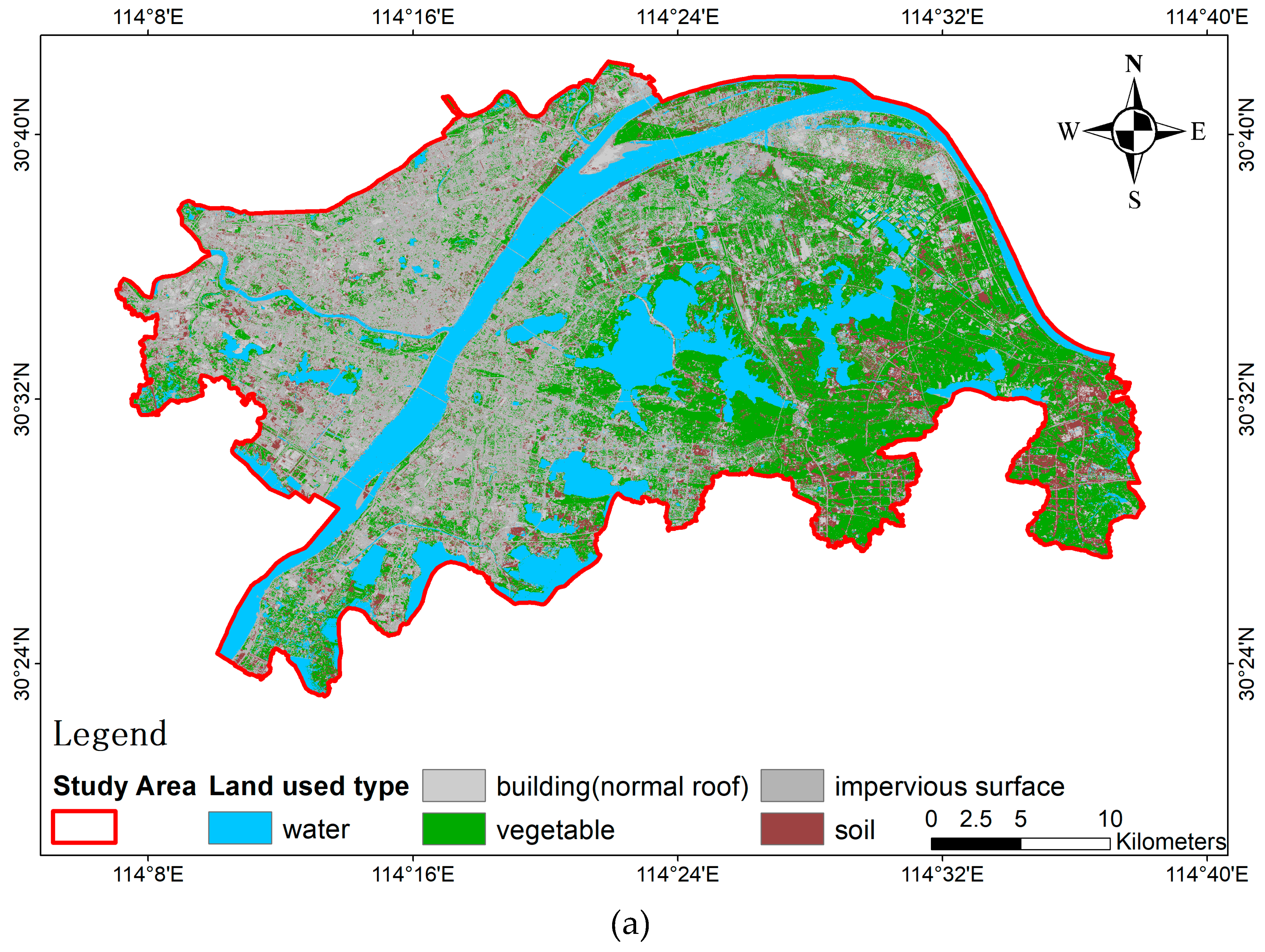
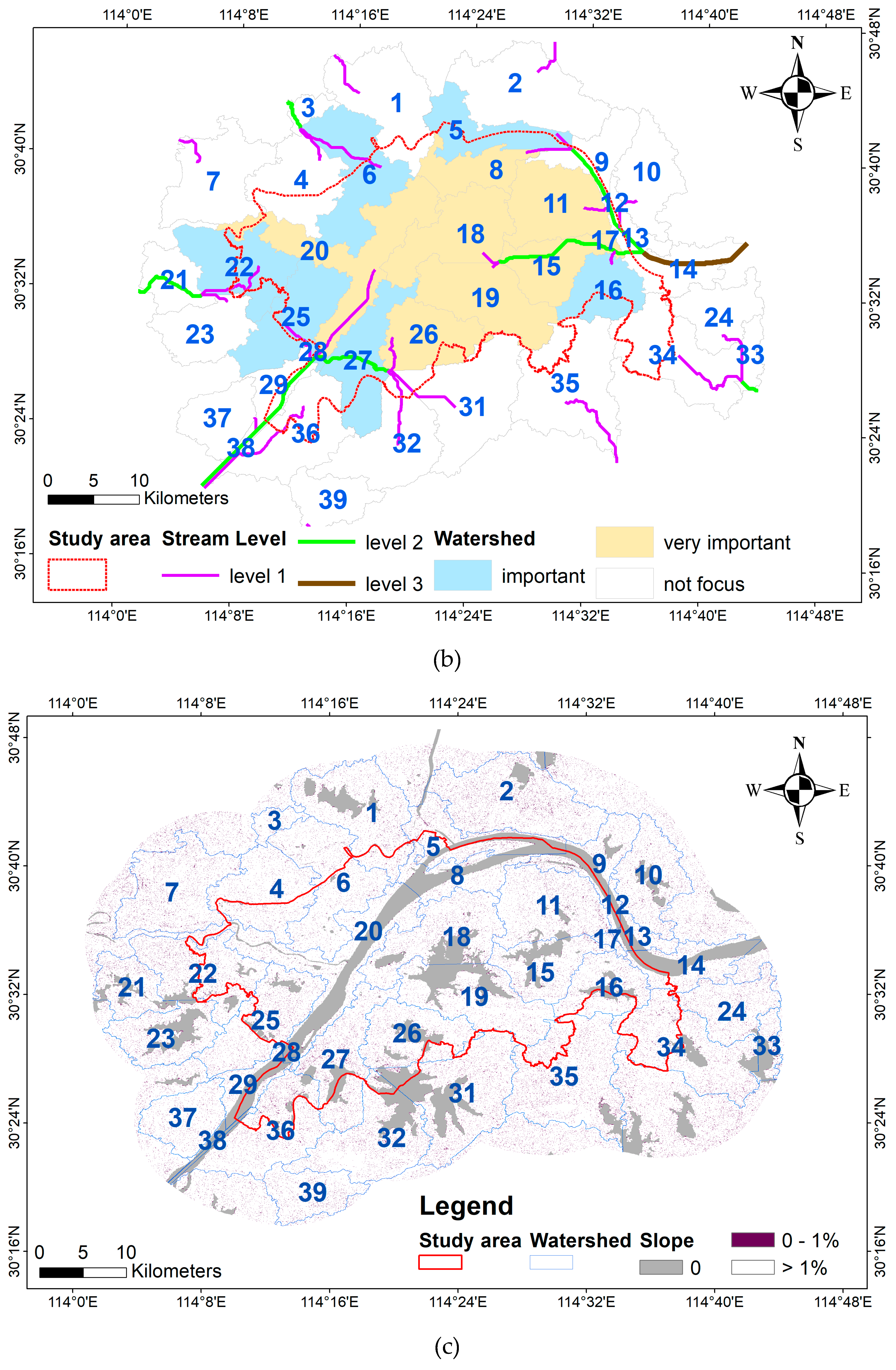
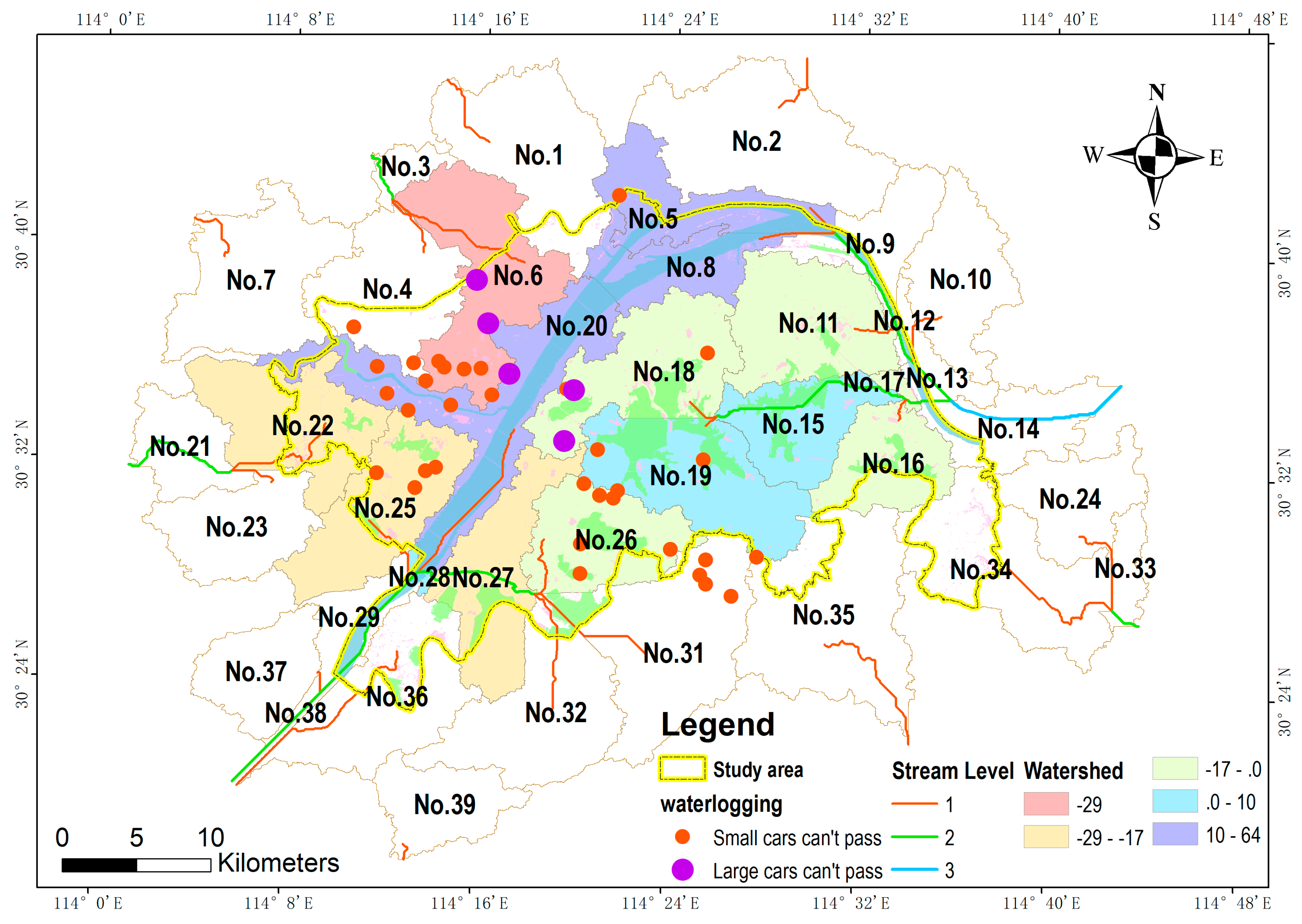
We mainly need to map the slope, land-use type, and the watershed, as shown in Figure 3. With the exception of the land-use type, which is extracted by ENVI 5.3, the other maps are produced using the related tools in ARCGIS 10.2.

1) Land-use type. The ratio of land cover type is used to calculate the rainfall–runoff production based on the urban runoff coefficient in each sub-watershed. The land cover type is composed of the vegetation, impervious surface, soil, and water, based on the VIS-W model. The maximum likelihood method was used to extract the land cover type by ENVI 5.3 from the GF-1 and GF-2 images. We firstly extracted the vegetation, impervious surface, soil, water, and shadow. Then, according to the spatial adjacency between the shadow and the water, we could identify the part of shadow which should belong to water, and we regarded the left part of shadows as the impervious surface. This might bring a slight overestimation of the impervious surface, but we considered this as acceptable because the rainwater produced by the overestimated impervious surface is too small to disturb the collected water.

2) Watershed. The watershed polygon is the defined basic evaluation unit. We used the hydrology tool of ARCGIS 10.2, which is based on the D8 algorithm, to delimitate watershed. Related to the previous research, we used a refined DEM by water body for watershed delimitation, since the performances will increase the certainty of flow direction and improve the accuracy of the delimited watershed compared to the original DEM [42]. The adopted water body was extracted from GF-1 and GF-2 by the previous land type map step. Based on the smallest area of the Sanjiaohu lake watershed [43], we used 11,111 (10 km²/ 30 m × 30 m ≈ 11,111) as the limitation of flow accumulation to extract the stream network, and we got 38 sub-catchments, finally. Considering the condition that the inside area ratio must be higher than 40%, there are 15 sub-catchments that have been chosen. They are divided into two groups: the “very important” group, for which the ratio is more than 89% (including No. 8, No. 11, No. 15, No. 17, No. 18, No. 19, No. 20, and No. 26), and the “important” group, for which the ratio is between 40% and 89% (including No. 5, No. 6, No. 16, No. 22, No. 25, No. 27, and No. 28).

3) Slope < 1%. The slope < 1% raster map is used to identify the low-lying area, and it will be used to analyze the areas which need to pump outside of the watershed. It is calculated by the DEM data set using the slope analysis tool and the raster calculation tool in ARCGIS 10.2.

(5) Construct basic indicators

(1) $V_{Capacity}$. Corresponding precipitation in each sub-catchment is used to express the storage capacity. It is composed of three parts: the river, the lake, and the puddle or pond.

$$V_{Capacity}=R\_V_{Capacity}+L_{V_{Capacity}}+P\_V_{Capacity}$$

(8)

where $V_{Capacity}$ (unit: m³) represents the rainwater storage, and the storage volume of the river, lake, and puddle or pond are represented by the $R\_V_{Capacity}$ (unit: m³), $L\_V_{Capacity}$(unit: m³), and $P\_V_{Capacity}$(unit: m³), respectively.

● River storage

The potential storage of a river is determined by the limitation of the water level in flood seasons. In this paper, we take three meters as the water level increase limitation based on the flood control water level of the Yangtze River and Han River. Equation (9) is used to calculate this storage capacity:

$$R\_V_{Capacity}={{\displaystyle \sum }}_1^n{A}_i\times \rho \times h \left(\rho =1.0, h=3.0\right)$$

(9)

where $R\_V_{Capacity}$_y (its unit is 10⁶ m³) represents the storage capacity of the river area in the sub-catchment, A_i (unit 10⁶ m³) is the area of water belonging to the river, ρ represents the area coefficient of the calculated river, and h (unit is m) is the storing water depth. We default set the following: ρ = 1.0 and h = 3.0.

● Lake storage

Zhou et al. [43] proposed the identification of the storage of lakes in terms of pre-regular pumping (the water level should be 0.3 m, and the area coefficient should be 0.8), normal storage (the water level should be 1 m, and the area coefficient should be 1), and extended water level (the water level should be 0.3 m, and the area coefficient should be 1.2).

$$\{\begin{array}{ll}\multicolumn{2}{c}{\mathrm{L}\_{\mathrm{V}}_{\mathrm{Capacity}}={\mathrm{V}}_{\mathrm{normal}}+{\mathrm{V}}_{\mathrm{pre}\_\mathrm{pumping}}+{\mathrm{V}}_{\mathrm{expansion}}}\\ {\mathrm{V}}_{\mathrm{normal}}={{\displaystyle \sum }}_1^{\mathrm{n}}{\mathrm{A}}_{\mathrm{i}}\times \mathsf{\rho }\times \mathrm{h}& \mathsf{\rho }=1.0,\mathrm{h}=1.0\\ {\mathrm{V}}_{\mathrm{pre}\_\mathrm{pumping}}={{\displaystyle \sum }}_1^{\mathrm{n}}{\mathrm{A}}_{\mathrm{i}}\times \mathsf{\rho }\times \mathrm{h}& \mathsf{\rho }=0.8,\mathrm{h}=0.3\\ {\mathrm{V}}_{\mathrm{expansion}}={{\displaystyle \sum }}_1^{\mathrm{n}}{\mathrm{A}}_{\mathrm{i}}\times \mathsf{\rho }\times \mathrm{h}& \mathsf{\rho }=1.2,\mathrm{h}=0.3\end{array}$$

(10)

Here, $L\_V_{Capacity}$ (unit: 10⁶ m³) represents the capacity of lake storage, $V_{normal}$ (unit: 10⁶ m³) represents the storage of a normal storage capacity, $V_{pre\_pumping}$ (unit: 10⁶ m³) represents the volume of the pre-regular pumping water level before flood seasons, and $V_{expansion}$ (unit: 10⁶ m³) represents the magnifying storage according to the surveyed average flood control water level. A_i (unit: 10⁶ m²) represents the area of lakes in the sub-catchment, ρ represents the calculating area coefficient of lakes, and h (unit: m) represents the permission increasing water level in lakes. We default set ρ = 1.0 and h = 1.0 to calculate the normal storage, set ρ = 0.8 and h = 0.3 to calculate the pre-pumping storage, and set ρ = 1.2 and h = 0.3 to calculate the lakes’ expansion storage.

● Puddle or pond storage

Puddles or ponds can temporarily store rainwater in residential areas. In this study, we defined single areas of water bodies measuring between 900 square meters and 100,000 square meters as puddle or pond entities. This is because 900 square meters represents an area of about the horizon resolution of DEM (length 30 meters, and width 30 meters). Additionally, the area of 100,000 square meters is close to the area of Sanjiao Lake, which is the smallest lake in Wuhan. The distribution of pits or ponds is wide and relatively separate. We found the location of pits or ponds to be generally near residents, which demonstrated that there is no room to extend the water level higher than the shores. We default set the average increase in water level as 0.8 m.

$$P\_V_{Capacity}={{\displaystyle \sum }}_1^n{A}_i\times \rho \times h(\rho =1.0, h=0.8)$$

(11)

Here, $P\_V_{Capacity}$ (unit: 10⁶ m³) represents the storage, A_i (unit: 10⁶ m²) represents the area of the puddle or pond in the sub-catchment, ρ represents the area coefficient for calculating the puddle or pond, and h (unit: m) represents the water level. We default set ρ = 1.0 and h = 0.8.

● The storage capacity identify by the interval of rainfall intensity

According to the pre-defined runoff coefficient, the integrated runoff coefficient by land cover type area in each catchment can be estimated according to Equation (6). Finally, the storage capacity of each sub-catchment can be calculated as follows:

$$R_{Int}=R_{Int\left(12h\right)} or R_{Int\left(6h\right)} ,Precipitation=1000\times \frac{\raisebox{1ex}{$V_{Capacity}$}\!\left/ \!\raisebox{-1ex}{$Area$}\right.}{{\Psi }_{int}}$$

(12)

where the rainfall intensity $Precipitation\left(\mathrm{unit}:\mathrm{mm}\right)$ is restricted by the rainwater storage $V_{Capacity}$ (unit: m³); the area of sub-catchment is recorded as $Area$(unit: m²); and the integrated runoff is the coefficient ${\Psi }_{int}$. $R_{Int\left(12h\right)}$ or $R_{Int\left(6h\right)}$ represent the precipitation of a certain return period interval, which is calculated by Equation (7).

(2) Ai. This represents the area of vegetation, soil, impervious surface, and water. It can be calculated by the statistical analysis tool in ARCGIS 10.2. The sub-catchment polygon is used to extract the area of vegetation, soil, impervious surface, and water from the land used type raster by the geometry analysis function in ARCGIS 10.2.

(3) $F_{Low}$. The ratio of low-lying areas represents the area for which the slope is less than 1%, except the area for which the land cover type is water.

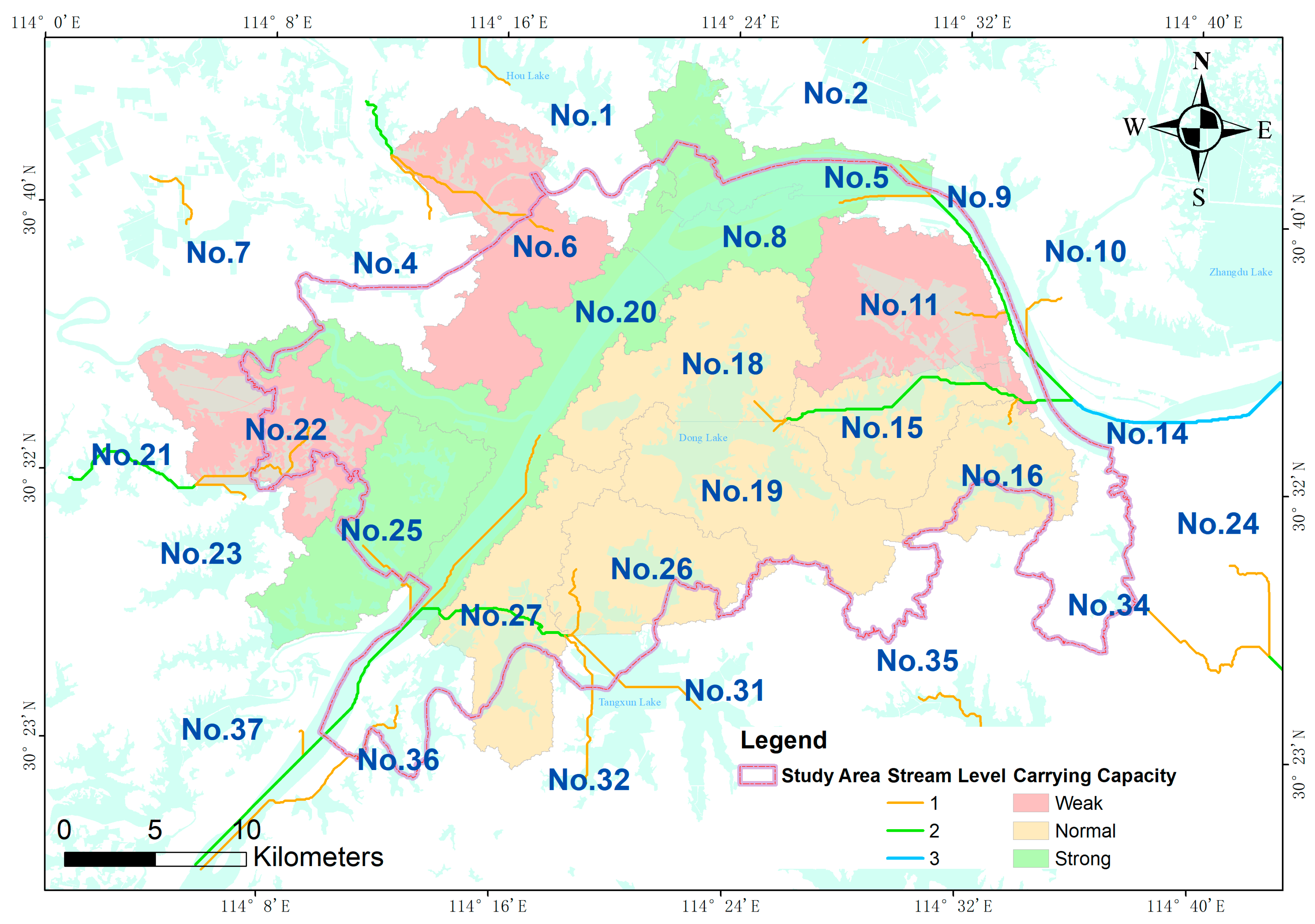
(4) $L_{River}.$ The stream level represents the flow path inside the urbanized catchment. It adopts the river level function in the hydrology analysis tool in ArcGIS 10.2 to calculate its value, using the stream data extracted from the flow accumulation raster. The level of stream is named according to the Strahler level definition, which adopts the river link to the stream level from upstream to downstream. When the branches with the same grade of streams converge together, the level of current link will move up one grade, otherwise, the higher value is kept among its branches.

(5) $F_{Terminaltype}$. The terminal flow type of the sub-watershed current is analyzed by the stream link and the flow path. It is labeled as “river” “inner”, and “outer”. The term “river” represents the downstream link finally pouring into river and the term “outer” represents the downstream link finally pouring outside of the catchment; otherwise, the terminal flow type can be labeled as “inner”.

(6) $F_{Nexttype}$. The sub-catchment of the next flow type represents the type of neighbor sub-catchment along the flow path. It is also labeled as “river”, “inner”, and “outer”.

(7) $Len(F_{Outlet})$. The length is from current sub-catchment to the main outlet. In this paper, it is used to record the sub-watersheds to the river. If the terminal flow type is “outlet”, the value of $Len(F_{Outlet})$ shall use a value twice the $Len(F_{Outlet})$ maximum values among the sub-watersheds for which the terminal flow types are labeled as “river” or “inner”.

(8) $Count\left(F_{Areas}\right)$. The count of sub-catchment follows the flow path from upstream. Its value is default set as 1, which means that the area only receives rainwater from itself.

Finally, all of the basic indicators in each sub-catchment are listed in

Table 6. The basic indicator used in the study area for flood capacity assessment.

Catchment	VCapacity		FLow	LRiver	FTerminaltype	FNexttype	Len(FOutlet)	$\mathit{C}\mathit{o}\mathit{u}\mathit{n}\mathit{t}$ $\left({\mathit{F}}_{\mathit{A}\mathit{r}\mathit{e}\mathit{a}\mathit{s}}\right)$	Ai
	${\mathit{R}}_{\mathit{I}\mathit{n}\mathit{t}\left(6\mathit{h}\right)}$	${\mathit{R}}_{\mathit{I}\mathit{n}\mathit{t}\left(12\mathit{h}\right)}$							(water)
No.5	>100	>100	1.08	1	river	river	1	1	0.38
No.6	<1	<1	0.81	1	outer	outer	6	1	0.02
No.8	>100	>100	0.68	1	river	river	0	1	0.32
No.11	1–5	5–10	1.14	1	river	river	1	1	0.07
No.15	~100	20–100	0.97	2	river	inner	2	3	0.2
No.16	20–100	20~100	0.84	1	river	inner	2	1	0.12
No.17	<1	<1	1.48	3	river	river	1	5	0.03
No.18	20–100	20–100	0.95	1	river	inner	3	1	0.18
No.19	~100	20~100	0.77	1	river	inner	3	1	0.23
No.20	>100	>100	0.55	1	river	inner	0	1	0.34
No.22	1–5	5–10	1.21	1	outer	inner	6	1	0.08
No.25	20–100	20–100	1.06	1	river	river	1	1	0.13
No.26	20–100	20–100	1.01	1	river	inner	2	1	0.17
No.27	20–100	20–100	1.27	2	river	river	1	4	0.12
No.28	>100	>100	0.90	2	river	river	0	7	0.51

.

3. Results

According to the proposed model, the urban flood-carrying capacity can be derived by the storing ability, the receiving ability, the drainage potential, and the pumping emergency. The flood-carrying capacity estimating result is shown in

Table 7. Urban flood-carrying capacity assessment in the study area.

Index	Catchment	Storing Ability	Receiving Ability	Drainage Potential	Pumping Emergency	Flood-carrying Capacity
1	No.5	very strong	very strong	very strong	normal	strong
2	No.6	very weak	very weak	weak	urgent	weak
3	No.8	very strong	very strong	very strong	not urgent	strong
4	No.11	weak	weak	strong	normal	weak
5	No.15	strong	strong	normal	urgent	weak
6	No.16	strong	strong	normal	normal	normal
7	No.17	very weak	very weak	strong	urgent	weak
8	No.18	strong	strong	normal	normal	normal
9	No.19	strong	very strong	normal	normal	normal
10	No.20	very strong	very strong	very strong	not urgent	strong
11	No.22	very weak	weak	very weak	urgent	weak
12	No.25	strong	strong	strong	normal	normal
13	No.26	strong	normal	normal	normal	normal
14	No.27	normal	normal	strong	urgent	weak
15	No.28	very strong	strong	very strong	not urgent	strong

. We find that the previous three abilities are summarized strictly by the lowest level, and the pumping emergency has the highest prior affectation in the final estimation results. The final result will be moved down one grade by the state of emergency compared with the previous three abilities combined. The state of “not urgent” keeps the original level unchanged. Taking No.5 and No.25 for example, for both the pumping emergency is labeled as “normal”. Meanwhile, the original levels of No.5 and No.25 are “very strong” and “strong”, respectively. Therefore, the finally flood-carrying capacities are “strong” and “normal”, respectively.

As shown in Table 7, there are four, five, and six sub-catchments whose capacities are labeled as “strong”, “weak”, and “normal”, respectively. Figure 4 shows the distribution of the flood-carrying capacity. We can determine that the “strong” sub-catchment (e.g., No.5, No.8, No.20, and No.28) contains a part of river area. We can also find that the flood-carrying capacity is determined by the distance to the outlet, its rain water storage advantage, the receiving demand along the stream flow, and its low-lying areas. For example, comparing the distance to the river, both sub-catchments No.25 and No.27 neighbor the river, but the final state of No.25 is normal, and that of No.27 is weak. As we can see in Figure 4, sub-catchment No.27 is located downstream of the flow path and it needs to receive the rainwater from upstream, including sub-catchment No.26, No.31, and so on; meanwhile, the stream level of No.25 is first, meaning it is located at the beginning of stream. The flood-carrying capacity of No.25 is better than that of No.27.

4. Discussion

4.1. Comparing the Carrying Capacity with Waterlogging Points

According to the rainfall intensity during 12-hour in Wuhan shown in Table 4, the return period value in 5–20 years is 107.35–171.85 mm, and the return period values for 5 years, 20 years, and 100 years are 138.1 mm, 205.6 mm, and 336.2 mm, respectively. In the flood disaster from 30 June to 6 July 2016, the cumulative precipitation value on severe days was 583.1 mm, according to the precipitation record of Station No. 57,494. The cumulative precipitation passed the limitations of the 100-year return period.

Indeed, as per the waterlogging point distribution released by Wuhan officials on July 6, 2016 (http://www.whwater.gov.cn/water/fxkht/7958.html, accessed: November 5, 2017), this flood and waterlogging event caused 99 waterlogging places in central Wuhan city, and all the water depths are too high to be convenient for motor vehicles to pass through. Inside Third Ring Road of Wuhan, there were 40 waterlogging points not suitable for motor vehicles to pass through, as shown in Figure 5. We found that 30 of them were located in the range of the study area. These points were grouped as “large cars cannot pass” and “small cars cannot pass”. Here, “large cars” refer to large vehicles like buses and trucks, as compared to small household cars. The points labeled as “large car cannot pass” indicate none of the cars can pass through, while in the “small car cannot pass” range, only the large cars can pass through. As shown in Figure 5, there are a total of eight sub-catchments located inside Third Ring Road of Wuhan. The flood-carrying capacity in two of them are “weak”, four of them are “normal”, and the remaining two are “strong”. On comparing the waterlogging distribution to the flood-carrying capacity of sub-watersheds, one of the “weak” sub-catchments (No.6) suffering from waterlogging was labeled as “large car cannot pass” and “small cars cannot pass”, and one of the “normal” sub-catchments (No.18) has the same situation as No.6. There are four “normal” sub-catchments (No.19, No.20, No.25, and No.26) which have waterlogging points labeled as “small car cannot pass”. Furthermore, there was one “strong” sub-catchment (No.8) and one “weak” sub-catchment (No.27) that did not have waterlogging point, respectively. The accumulative waterlogging points of three level are listed in

Table 8. The typical waterlogging points distribution inside Third Ring Road of Wuhan. As listed in the number of sub-catchments, there are eight sub-catchments inside Third Ring Road, and there are two sub-catchments that have no waterlogging points. The columns “Large car cannot pass” and “Small car cannot pass” indicate different depths of waterlogging points, where the depth in the former is higher than in the latter. The distribution of waterlogging section lists the quality of points in three classes of sub-catchment, respectively.

Label	Amount of Sub-Catchments				Distribution of Waterlogging
	Total	No Waterlogging	Large Car Cannot Pass	Small Car Cannot Pass	Total	Large Car Cannot Pass	Small Car Cannot Pass
weak	2	1	1	1	9	3	6
normal	4	0	1	3	17	2	15
strong	2	1	0	1	4	0	4

.

According to the statistical waterlogging points in Table 7, we can find that firstly, in terms of the sub-watershed, 100% of the “large cars cannot pass” waterlogging points occurred in the “weak” or “normal” sub-catchments. We also noticed that in the two sub-catchments for which the flood-carrying capacity level is “weak”, No.27 had no waterlogging points. Compared to the real drainage pumping station, the Tangxun Lake pumping station is located in No.27, and it fully runs during the flood days. This may be the reason that this “weak” area met no waterlogging points at all. We can also see that 80% of the waterlogging points labeled as “small cars cannot pass” took place in the “weak” and “normal” sub-catchments, but there are still some waterlogging points in the “strong” sub-catchment (No. 20). Secondly, in terms of the numbers of waterlogging points, as shown in Figure 6, we can see that 84% of the points located in the “weak” and “normal” sub-watershed, and 100% of the points labeled “large cars cannot pass” were located in the “weak” or “normal” sub-watersheds. As the accumulative precipitation nearly passed the return period of 100 years during the flood and waterlogging event, the waterlogging points which take place in areas with flood-carrying capacities of “weak” or “normal” are understandable.

Generally, over 80% of the typical waterlogging points are located in area whose flood-carrying capacity states are “weak” or “normal”. This statistical result indicates the urban flood-carrying capacity estimated by the proposed model is reasonable, and the proposed model can be used to estimate the urban flood-carrying capacity.

4.2. Discussion on the Storing Ability of Each Sub-Catchment in the Waterlogging Event

We further analyzed the potential capacity of the natural water system according to the flood and waterlogging disaster event. Based on the hydrological observation data, from 00:00 h on 30 June 2016 to 00:00 h on 12 July 2016 (Station: Hankou Station), we found that the original water level of Yangtze River on 30 June 2016 was 25 m, and the maximum level reached 28.37 m at 04:00 h on 7 July 2016. This record verified that the storage rainwater ability of the Yangtze River can be calculated by the increase in the limitation water level of 3 m. Additionally, the increased water level in the lakes in the direct pre-regular plan is 1 m, the normal rising level is 0.3 m, and the extended flood control level is 0.3 m, according to the flood control for Wuhan proposed in the literature [43].

We finally calculated the result of the quantity of runoff based on the rainfall–runoff hydrological model by integrating the runoff coefficient of the underlying surface, which was about 235 million m³ in the flood and waterlogging disaster event which occurred from 30 June 2016 to 6 July 2016. Meanwhile, the whole storage capacity was about 298 million m³. Therefore, the total balance of the flood-carrying capacity is higher than that of the runoff rainwater. In theory, the whole city can avoid waterlogging if the storing capacity can be regulated as freely as possible.

As shown in Figure 7, the rainwater storage capacities in the waterlogging disaster in sub-catchments No.6 (in red color), No.22, No.25, and No.27 (in light brown colors), and No.11, No.18, No.16, No.17, and No.26 (in light green colors), are overloaded. The storage capacities of sub-catchments No.15 and No.19 in light blue color are slightly greater than the quantity of rainwater. Furthermore, the storage capacities in No.5, No.8, and No.20 (in light purple colors) are much higher than the quantity of rainwater.

Compared to the self-container storage capacity in the sub-catchment, the seven waterlogged places located in No.5, No.8, and No.20, and the three waterlogged places located in No.19, are not reasonable. The waterlogged places located in No.25, No.26, and No.18 can be understood in terms of the natural water system as having a lesser capacity compared to the quantity of rainwater. The five waterlogged places located in the No.6 sub-catchment are reasonable. This is because the local storage of the natural water entity is not plentiful. According to the stream network, the flow path of the sub-catchment is finally outside of the study areas whose direction is opposite to the main outlet of the Yangtze River or Han River.

In our opinion, the waterlogging disaster could have been mitigated by a combination of fully using the natural drainage capacity and a reasonable drainage schedule of the city. According to the standards of the Wuhan government, if there exists waterlogging of higher than 0.4 m for more than 2 h, the level of waterlogging can be defined as serious. In the serious flood and waterlogging disaster used in this paper, we believe the ability to regulate the natural water system is not sufficient. Taking catchment No.26 as an example, the longest duration of waterlogging is located here. From the city’s drainage network, the rainwater naturally flows to No.27 and is finally pumped into the Yangtze River at the Tangxun lake pump station. During the waterlogging event, sub-catchment No.26 produced about 22 million m³ of runoff rainwater, and its maximum regulated storing capacity is 13 million m³. Therefore, there remained 9 million m³ of rainwater that needed to be discharged. According to the official information, the designed drainage capacity of the Tangxun Lake pump station is 120 m³/s, which means that the pump system needs to work for about 21 h to pump rainwater into the city’s drainage system. However, in the pump work report, the Tangxun Lake pump station ran for 90 h from July 1 to 6. Meanwhile, we have found that there are six waterlogging places located in sub-catchment No.26.

4.3. Analyzing the Carrying Capacity with Land Type and Terrian Factors

According to the estimation model expressed in Section 2.3, we can see that the urban flood-carrying capacity corresponds with the underlying surface. For example, the terrain characteristics will affect the delimitation of the watershed and influence the flow path. The land cover type will determine the ratio of runoff yield, and the potential of discharge will affect the degree of waterlogging risk. As shown in Figure 8, we adopted statistical graphs to discuss the relation between the estimated results and the underlying surface characteristics. Figure 8a,b used the main axis on the left to display comparison factors (land cover type ratio, storing ability transforming into precipitation measured by runoff yield, elevation range, and slope), and adopted “1”, “2”, and “3” to map the carrying capacity states of “weak”, “normal”, and “strong”, respectively, by the secondary axis.

Figure 8a uses the cumulative ratio of land use type to draw a histogram chart. In Figure 8a, we can find that the “weak” areas always have a similar shape to areas with a low ratio of the water body, while most of the “strong” areas are similar to those with a high ratio of the water body. Furthermore, the “normal” areas are not very significant in terms of the proportion of water. These phenomena indicate that the flood-carrying capacity of each sub-catchment is positively correlated with the water ratio. Moreover, the water area is the land cover of open water extracted by the remote sensing images. This indicates that the carrying capacity can reflect the storing rainwater ability to regulate the natural water system.

Figure 8b uses the logarithmic function with a base of 2 to pre-calculate the underlying surface factors, and finally displays the results as a line chart. In Figure 8b, we used two kinds of terrain factors (ratio of slope < 1% areas and elevation range) and one kind of rainfall factor (runoff) for analysis. Both of the terrain factors reflect the change of elevation from different aspects. The slope is the average value of elevation, which shows the local land relief character, and can distinguish the ratio of low-lying areas. The elevation range is the regional topographic drop, and can reflect the flow path of rainwater. The line shape and the amplitude of terrain factors are different. From Figure 8b, we can find that the storing runoff ability is similar to the shape of the slope to a certain degree. The reason for this is that the ratio of low-lying land is an indicator of the storing ability. Additionally, the area with a “high” carrying capacity always has a peak value of storing ability of runoff. Sub-catchment No.25 does not have not the local peak runoff ability, but its slope of less than 1% is low and the elevation range is very high, which shows that the area might flow into a neighboring area. Therefore, its flood-carrying capacity is “strong”. The phenomenon indicates that the estimating model is synthesized considering the water areas, runoff coefficient, and flow path.

5. Conclusions

The study proposed a novel model based on the underlying surface VIS-W model to estimate the urban flood-carrying capacity in terms of the consistency with the land use type, the terrain features, the storage, receiving and discharge ability, and pumping outward emergency of the natural water system, through (1) extending the VIS underlying surfaces model to form the VIS-W model, (2) delimiting the sub-watershed of the urban catchment by DEM data set constrained by the water body, and (3) calculating the rainwater budget with the storage capacity of rivers, lakes, and puddles or ponds in each sub-catchment by a rainfall–runoff model; combined with the hydrological features of the terrain, the flood-carrying capacity could be comprehensively derived.

On comparing to the verified result with the flood-carrying capacity and typical waterlogging points inside Third Ring Road of Wuhan, we found 80% of sub-catchments with flood-carrying capacity categorized as “weak” or “normal” suffered waterlogging disasters, and 84% were located in sub-watersheds labeled as “weak” or “normal”. This proves that the proposed model could be suitable for estimating the flood-carrying capacity in cities like Wuhan. Furthermore, on comparing the surplus state of the storing ability, the inconsistency between the waterlogging places and the flood-carrying capacity indicated that the storing ability might have some space for improvement. In our opinion, waterlogging disasters might be mitigated by fully utilizing the natural storage capacity to coordinate the normal flood drainage schedule.

In future research, the potential for regulating the natural water system in urbanized catchments should be analyzed. Additionally, rainfall scenes simulated by 1D or 2D hydrodynamic models should be overlapped to analyze the drainage performances.

References

1. Guha-Sapir, D.; Hoyois, P.; Wallemacq, P.; Below, R. Annual Disaster Statistical Review 2016; CRED: Brussels, Belgium, 2016; pp. 1, 19. [Google Scholar]
2. CMA. The National Disaster Reduction Statistics Report in 2016. Available online: http://www.mca.gov.cn/article/zwgk/mzyw/201701/20170100002965.shtml (accessed on 16 November 2017). (In Chinese)
3. Zhang, J.; Wang, Y.; He, R.; Hu, Q.; Song, X. Discussion on the urban flood and waterlogging and causes analysis in China. Adv. Water Sci. 2016, 27, 485–491. [Google Scholar]
4. Xu, Z.; Chen, T.; Ren, M. “City Ocean”: Urban hydrological challenges and opportunities. China Flood Drought Manag. 2017, 5, 64–66. (In Chinese) [Google Scholar]
5. Zhang, Y.; Li, H.; Reggiani, P. Climate variability and climate change impacts on land surface, hydrological processes and water management. Water 2019, 11, 1492. [Google Scholar] [CrossRef]
6. Zhou, D.; Zhao, S.; Zhang, L.; Liu, S. Remotely sensed assessment of urbanization effects on vegetation phenology in China’s 32 major cities. Remote Sens. Environ. 2016, 2016, 272–281. [Google Scholar] [CrossRef]
7. Yang, L.; Smith, J.A.; Wright, D.B.; Baeck, M.L.; Villarini, G.; Tian, F.; Hu, H. Urbanization and climate change: An examination of nonstationarities in urban flooding. J. Hydrometeorol 2012, 14, 623–631. [Google Scholar] [CrossRef]
8. Locatelli, L.; Mark, O.; Mikkelsen, P.S.; Arnbjerg-Nielsen, K.; Deletic, A.; Roldin, M.; Binning, P.J. Hydrologic impact of urbanization with extensive stormwater infiltration. J. Hydrol. 2017, 544, 524–537. [Google Scholar] [CrossRef] [Green Version]
9. Barasa, B.N.; Perera, E.D.P. Analysis of land use change impacts on flash flood occurrences in the Sosiani River basin Kenya. Int. J. River Basin Manag. 2018, 16, 179–188. [Google Scholar] [CrossRef]
10. Zhang, L.; Zhang, M.; Yao, Y. Mapping seasonal impervious surface dynamics in Wuhan urban agglomeration, China from 2000 to 2016. Int. J. Appl. Earth Obs. 2018, 70, 51–61. [Google Scholar] [CrossRef]
11. Zhu, J.; Zhang, Q.; Tong, Z. Impact analysis of lakefront land use changes on lake area in Wuhan, China. Water 2015, 7, 4869–4886. [Google Scholar] [CrossRef]
12. Deng, Y.; Jiang, W.; Tang, Z.; Li, J.; Lv, J.; Chen, Z.; Jia, K. Spatio-temporal change of lake water extent in wuhan urban agglomeration based on landsat images from 1987 to 2015. Remote Sens. 2017, 9, 270. [Google Scholar] [CrossRef]
13. Huang, Z.Y.; Peng, T.; Zhang, H.Y.; Yao, W.L. Study of risk and early warning index of rainstorm waterlogging in Wuhan City. In Proceedings of the 3rd International Conference on Water Resource and Environment (WRE 2017), Qingdao, China, 26–29 June 2017; Li, P., Ed.; IOP Publishing Ltd.: Qingdao, China, 2017. [Google Scholar]
14. Chen, X. Analysis on the causes of systematic waterlogging of Tangxun Lake and Nan Lake region in Wuhan city. China Water Wastewater 2017, 33, 7–10. [Google Scholar]
15. Xia, J.; Shi, W.; Wang, Q.; Zou, L. Discussion of several hydrological issues regarding sponge city construction. Water Resour. Prot. 2017, 33, 1–8. [Google Scholar]
16. Rezende, O.M.; Miranda, F.M.; Haddad, A.N.; Miguez, M.G. A framework to evaluate urban flood resilience of design alternatives for flood defense considering future adverse scenarios. Water 2019, 11, 1485. [Google Scholar] [CrossRef]
17. General Office of the State Council. Office of the state council guiding opinions of the general office of the state council on promoting the construction of sponge city. Water Feild 2015, 6, 4–6. (In Chinese) [Google Scholar]
18. Zevenbergen, C.; Fu, D.; Pathirana, A. Transitioning to sponge cities: Challenges and opportunities to address urban water problems in China. Water 2018, 10, 1230. [Google Scholar] [CrossRef]
19. Sang, Y.; Yang, M. Urban waterlogs control in China: More effective strategies and actions are needed. Nat. Hazards 2017, 85, 1291–1294. [Google Scholar] [CrossRef]
20. Ning, Y.; Dong, W.; Lin, L.; Zhang, Q. Analyzing the causes of urban waterlogging and sponge city technology in China. IOP Conf. Ser. Earth Environ. Sci. 2017, 59, 12047. [Google Scholar] [CrossRef]
21. Li, B.; Dong, S.; Huang, Y.; Wang, G. Development of a heterogeneity analysis framework for collaborative sponge city management. Water 2019, 11, 1995. [Google Scholar] [CrossRef]
22. Zheng, Z.; Gao, J.; Ma, Z.; Wang, Z.; Yang, X.; Luo, X.; Jacquet, T.; Fu, G. Urban flooding in China: Main causes and policy recommendations. Hydrol. Process. 2016, 30, 1149–1152. [Google Scholar] [CrossRef]
23. Chen, K.; Wang, X.; Li, D.; Li, Z. Driving force of the morphological change of the urban lake ecosystem: A case study of Wuhan, 1990–2013. Ecol. Model. 2015, 318, 204–209. [Google Scholar] [CrossRef]
24. Wang, W.; Pilgrim, M.; Liu, J. The evolution of river-lake and urban compound systems: A case study in Wuhan, China. Sustainability 2016, 8, 15. [Google Scholar] [CrossRef]
25. Bhowmik, N.G.; Demissie, M. Carrying capacity of flood plain. J. Hydraul. Div. ASCE 1982, 108, 443–452. [Google Scholar]
26. Buehler, B.; ASCE, F. Discussion of “Carrying capacity of flood plains”. J. Hydraul. Eng. 1983, 109, 643–644. [Google Scholar] [CrossRef]
27. Qu, P.; Huang, R. Flood Carrying Capacity Analysis of Xinyihe River. In Proceedings of the 1st International Yellow River Forum, Zhengzhou, China, 12–15 May 2003; Shang, H.Q., Ed.; Yellow River Conservancy Press: Zhengzhou, China, 2003; pp. 417–420. [Google Scholar]
28. Shi, C.; Liu, J.; Zhang, Y. Flood carrying capacity and characteristic flow (water level) of the middle and lower reaches of Weihe river in 2009. J. Water Resour. Water Eng. 2009, 20, 129–132. [Google Scholar]
29. Islam, M.T.; Baki, A.B.M.; Hossain, M.M.; Mahalder, B.; Kafi, M.A.H.; Parvin, B. An assessment of Carrying Capacity of Dhaleshwari River using HEC-RAS Model. Dhaka Univ. J. Sci. 2009, 57, 47–50. [Google Scholar]
30. Stoica, F.; Rosu, I.; Sofronie, C.; Dulau, R.; Sarb, M. Study regarding delineation of flood hazard zones in the hydrographic basin of the Somes River, Border area. Aerul si Apa. Componente ale Mediului; Air Water Compon. Environ. 2014, 2014, 264–269. [Google Scholar]
31. Seidl, I.; Tisdell, C.A. Carrying capacity reconsidered: From Malthus’ population theory to cultural carrying capacity. Ecol. Econ. 1999, 31, 395–408. [Google Scholar] [CrossRef]
32. Shelby, B.; Heberlein, T.A. Carrying Capacity in Recreation Settings; Oregon State University Press: Corvallis, OR, USA, 1986. [Google Scholar]
33. Khanna, P.; Babu, P.R.; George, M.S. Carrying-capacity as a basis for sustainable development a case study of National Capital Region in India. Prog. Plann. 1999, 52, 101–166. [Google Scholar] [CrossRef]
34. Khalequzzaman, M. Underlying causes of the Haor flood in 2017 in Bangladesh. In Proceedings of the Special Conference on Floods Waterlogging and Landslides in Bangladesh, Dhaka, Bangladesh, 4 February 2019. [Google Scholar]
35. Sriyana, I. Evaluation of watershed carrying capacity for watershed management (a case study on Bodri watershed, Central Java, Indonesia). MATEC Web Conf. 2018, 195, 5003. [Google Scholar] [CrossRef]
36. Wuhan Municipal People’s Government. The Overview of Wuhan city. Available online: http://www.wh.gov.cn/2018wh/zjwh_5785/whgk/ (accessed on 10 July 2019).
37. Bathrellos, G.D.; Skilodimou, H.D.; Chousianitis, K.; Youssef, A.M.; Pradhan, B. Suitability estimation for urban development using multi-hazard assessment map. Sci. Total Environ. 2017, 575, 119–134. [Google Scholar] [CrossRef]
38. Ouma, Y.; Tateishi, R. Urban flood vulnerability and risk mapping using integrated multi-parametric ahp and GIS: Methodological overview and case study assessment. Water 2014, 6, 1515–1545. [Google Scholar] [CrossRef]
39. Ren, B.Z. Study on the Urban Design Rainstorm and Rainfall Runoff Calculation Model. Ph.D. Thesis, Chongqing University, Chongqing, China, 2004. [Google Scholar]
40. Online Solicitation Opinions on “Wuhan Drainage and Flood Control System Planning and Design Standards”. Available online: http://zrzyhgh.wuhan.gov.cn/pc-6-51777.html (accessed on 4 September 2019). (In Chinese)
41. Hong, G.P.; Wan, J.; Liu, J.H.; Ye, H.M.; Xiang, H. Rainstorm waterlogging research on numerical simulation for short-duration in the urban area of Wuhan. Torrential Rain Disasters 2018, 12, 83–89. (In Chinese) [Google Scholar]
42. Zhang, H.; Cheng, X.; Zhao, D.; Ma, H. Analyzing the contribution of high resolution water range in dividing catchment based on D8 algorithm. In Proceedings of the IGARSS 2018–2018 IEEE International Geoscience and Remote Sensing Symposium, Valencia, Spain, 22–27 July 2018; IEEE: Valencia, Spain, 2018. [Google Scholar]
43. Zhou, Y.H.; Zhong, N.B.; Shi, Y.Q. Utilizing flood storage potential of lakes in Wuhan city (in Chinese). China Flood Drought Manag. 2015, 25, 18–21. [Google Scholar]
Figure 1. The study area comprises the downtown districts of Wuhan, Hubei Province, China, including the Jiang’an, Jianghan, Qiaokou, Hanyang, Wuchang, Hongshan, and Qingshan Districts.
Water 11 02345 g001
Figure 2. The urban flood-carrying capacity assessment process is made up of four steps. First, we extended the underlying surface model; second, we identified the parameters; third, we constructed the basic estimating maps and indicators; and finally, we estimated the urban flood-carrying capacity.
Water 11 02345 g002
Figure 3. The basic maps for estimating urban flood-carrying capacity. (a) The land-use type related to the structure of the VIS-W model. The building for which the roof is plastic or brick is extracted independently. The runoff coefficient of the impervious surface is adopted to calculate the final rainwater. (b) The watershed delimitation derived by the DEM data set constrained by the water body. (c) The area with slope less than 1%. It is colored in two classes: slope = 0 and 0 < slope < 1%.
Water 11 02345 g003aWater 11 02345 g003b
Figure 4. The flood-carrying ability of each catchment. The flood-carrying capacity is derived from the storing ability, the receiving ability, the drainage potential, and the pumping outward emergency.
Water 11 02345 g004
Figure 5. The typical waterlogging points distributed as overlapping the flood-carrying capacity result based on the actual data from the flood and waterlogging event which took place from 30 June to 6 July 2016. In the 30 waterlogging points, there were five points were not suitable for large motor vehicles to pass through, and 25 points were not suitable for small motor vehicles to pass through.
Water 11 02345 g005
Figure 6. The ratio of waterlogging points grouped by “small cars cannot pass” and “large cars cannot pass” according to the location in the sub-catchment with “weak”, “normal”, and “strong” capabilities.
Water 11 02345 g006
Figure 7. The waterlogging and carrying capacity in the flooding event in July 2016, showing the waterlogging sites overlapping with the estimated surplus storage of runoff rainwater.
Water 11 02345 g007
Figure 8. The urban flood-carrying capacity results comparing the factors of land-use type and terrain. (a) The comparison of land-use type. (b) The comparison of the elevation range of terrain, the slope, and the storing rainwater ability transforming as runoff.
Water 11 02345 g008