Linking Climate, Basin Morphology and Vegetation Characteristics to Fu’s Parameter in Data Poor Conditions

Abstract

The prediction of long term water balance components is not a trivial issue, even when empirical Budyko’s type approaches are used, because parameter estimation is often hampered by missing or poor hydrological data. In order to overcome this issue, we provided regression equations that link climate, morphological, and vegetation parameters to Fu’s parameter. Climate is here defined as a specific seasonal pattern of potential evapotranspiration and rain: five climatic scenarios have been considered to mimic different conditions worldwide. A weather generator has been used to create stochastic time series for the related climatic scenario, which in turn has been used as an input to a conceptual hydrological model to obtain long-term water balance components with low computational effort, while preserving fundamental process descriptions. The morphology and vegetation’s role in determining water partitioning process has been epitomized in four parameters of the conceptual model. Numerical simulations explored a large set of basins in the five climates. Results show that climate superimposes partitioning rules for a given basin; morphological and vegetation watershed properties, as conceptualized by model parameters, determine the Fu’s parameter within a given climate. A sensitive analysis confirmed that vegetation has the most influencing role in determining water partitioning rules, followed by soil permeability. Finally, linear regressions relating basin characteristics to Fu’s parameter have been obtained in the five climates and tested in a basin for each case, obtaining encouraging results. The small amount of data required and the very low computational effort of the method make this approach ideal for practitioners and hydrologists involved in annual runoff assessment.

1. Introduction

One of the most important challenges in hydrology is to quantify water availability for every climatic scenario and geographic area in order to support socio-economic activities and ecosystem needs [1].

Simplified models are available to explore water partitioning processes at large temporal and spatial scales [2,3,4]. Considering steady state conditions [5,6] and neglecting the variation of water storage [7,8,9], the mean annual precipitation $P$ is balanced by mean annual runoff $Q$ and mean annual evapotranspiration $ET$. Under these conditions, Budyko [10] found a semi-empirical relation between the ratio of mean annual potential evapotranspiration $E{T}_P$ to $P$ and the ratio of $ET$ to $P$. The first one is called the aridity index ($AI$) and it is an indicator related to the local climatic condition, meaning the higher the aridity index is, the dryer the climate. In the Budyko’s theory, $ET$ is constrained by energy and water availability, by net radiation, and by $P$ [11,12,13]. For this reason, the ratio of $ET/P$, called the evaporative index ($EI$), can vary between 0 and 1 (energy and water limit), differently to the aridity index that could be higher than one and theoretically could reach an infinite value.

The variability of Budyko’s curve could be caused by three main triggers [14]: (i) climate properties [15,16,17,18], (ii) catchments physical processes [19,20], and (iii) vegetation [6,21,22].

Different authors proposed parametric or analytic expressions to describe the relation between $EI$ and the aridity index $AI$ [5,23,24,25,26,27]; one of the most well known expressions was obtained by Fu [28] with only one parameter, commonly indicated as $\omega$, describing the rainfall partitioning into $Q$ and $ET$. The mathematical expression was as follows:

$$EI=\frac{ET}{P}=1+AI-{\left(1+A{I}^{\omega }\right)}^{1/\omega }.$$

(1)

The higher the Fu’s parameter, the higher $EI$ for a given aridity index $AI$. Some authors derived the $\omega$ value of Budyko’s semi-empirical expression as being equal to 2.6 [23,29,30].

Since Fu’s equation is a representation of Budyko’s curve that, as said before, is responsive to climate, catchment processes, and vegetation, $\omega$ should comprise and describe the variability in the annual water catchment response [8,30,31,32,33].

Different attempts have been done to interpret and model $\omega$. Using 270 Australian catchments, Zhang, Hickel, Dawes, Chiew, Western, and Briggs [9] performed a stepwise regression analysis between $\omega$ and basin properties (i.e., vegetation cover, precipitation characteristics, catchment slopes, and plant available water capacity), and found that the most significant elements were the average storm, depth, and coefficient of variation in daily precipitation. Similarly, Xu et al. [34] linked Fu’s parameter with geographic and morphometric catchment properties of a dataset composed by MOPEX “small” basins [35] and a “large basin” whose data are from different sources (CRU TS 3.20, HYDRO1K, GIMMS). A simple stepwise regression and a more complex artificial neural network analysis were adopted to explain the relationship between the $\omega$ hydrological defined parameter and morphological basin properties, finding good explanatory capacity of the two developed models for small and large basins ($R^2$ = 0.53–0.83). Latitude has proved to be the best correlate with Fu’s parameter. As an alternative, Yang et al. [36] selected non-linear expression for predicting $\omega$ over 180 non-humid basins in China, which was a function of infiltration capacity, soil water storage, and average terrain slope. The expression was able to predict annual water cycle components (95.2% and 62% of the variance of mean annual evapotranspiration and runoff, respectively) by just using the aforementioned morphological descriptors. Through water-soil-vegetation metrics, Abatzoglou and Ficklin [2] studied the correlation between $\omega$ and morphological properties over watersheds in the United States. The relative cumulative moisture surplus ($rCMS$), the ratio of available soil water holding capacity to precipitation ($AWC/P$), and the topographic slope were integrated in a regression model that demonstrated the ability to simulate the spatial variability of $\omega$ (81.2%), which was involved in increasing the value of $rCMS$ as Fu’s parameter decreased, whereas $AWC/P>0.4$ has direct proportionality with $\omega$.

In this work, we will trace an original way (i) to further demonstrate and support the idea that climate, basin morphology, and vegetation drive water partitioning within Budyko’s framework and (ii) to establish the $\omega$ value in data-poor condition, providing practitioners and hydrologists with a tool for assessing annual runoff. But, differently from the previous studies, we used in silico experiments. Namely, we ran a simple conceptual lumped model, which preserved the physical description of fundamental hydrological processes acting within a natural basin. The choice of a simple model allowed us to deal with a huge amount of stochastic input data, consider a large range of basin descriptors and vegetation types, and work within reasonable computational time. The model will be forced by stochastic synthetic potential evapotranspiration and precipitation daily timeseries. The climatic input will be generated by a weather generator that roughly epitomizes the climatic variability by using five combinations of seasonal patterns involving potential evapotranspiration and precipitation. The model parameters domain was explored in order to assess how basin morphology and vegetation impact on the water partitioning process and for determining the $\omega$ value. Then we interpreted the model outputs within the Budyko’s framework to unravel the role of climate, basin morphology, and vegetation in multi-years water partitioning rules.

2. Methods

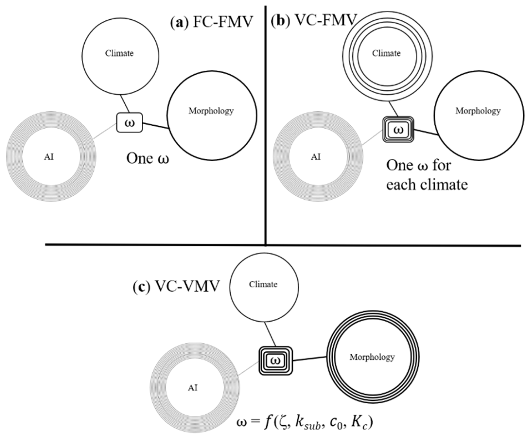
The role of climate, basin morphology, and vegetation in characterizing long term hydrological processes and in determining the $\omega$ value was explored by three consequent modeling experiments, which are sketched in Figure 1.

Supposing a particular climate, defined as a characteristic seasonal pattern of potential evapotranspiration and precipitation, once defined the morphological basin and vegetation properties (model parameters), we hypothesize that the hydrological response is only related to the aridity index. In other words, for a given climate condition, notwithstanding that the combinations between mean annual precipitation and potential evapotranspiration are infinite, water partitioning rules are uniquely defined. In the Budyko’s framework and using the Fu’s equation, this means that for different casual couples of $AI$ and $EI$, a unique value of $\omega$ is identifiable (Figure 1a).

Another cornerstone of this work is to support the idea that the hydrological behavior of a basin is driven by climate, again defined as a seasonal pattern of potential evapotranspiration and precipitation. Namely, the same basin (the same model parameters and then, morphological and vegetation properties), in different geographic areas with different seasonal patterns of climatic variables will result in different partitioning rules as a function of climate (Figure 1b).

Finally, we support the idea of biunivocal relationship between basin morphometric and vegetation properties and hydrological response (Figure 1c). Numerical simulations were run for the five climates with different basin morphological and vegetation properties (model parameter combinations). Results were used to create five linear relations (one for each climate type) between model parameters (that are four, representing the role of morphology and vegetation) and $\omega$. These relations are aimed to help practitioners and hydrologists in using Fu’s parameter in the case of limited or missing evapotranspiration and runoff data.

2.1. Climatic Scenarios and Weather Generator

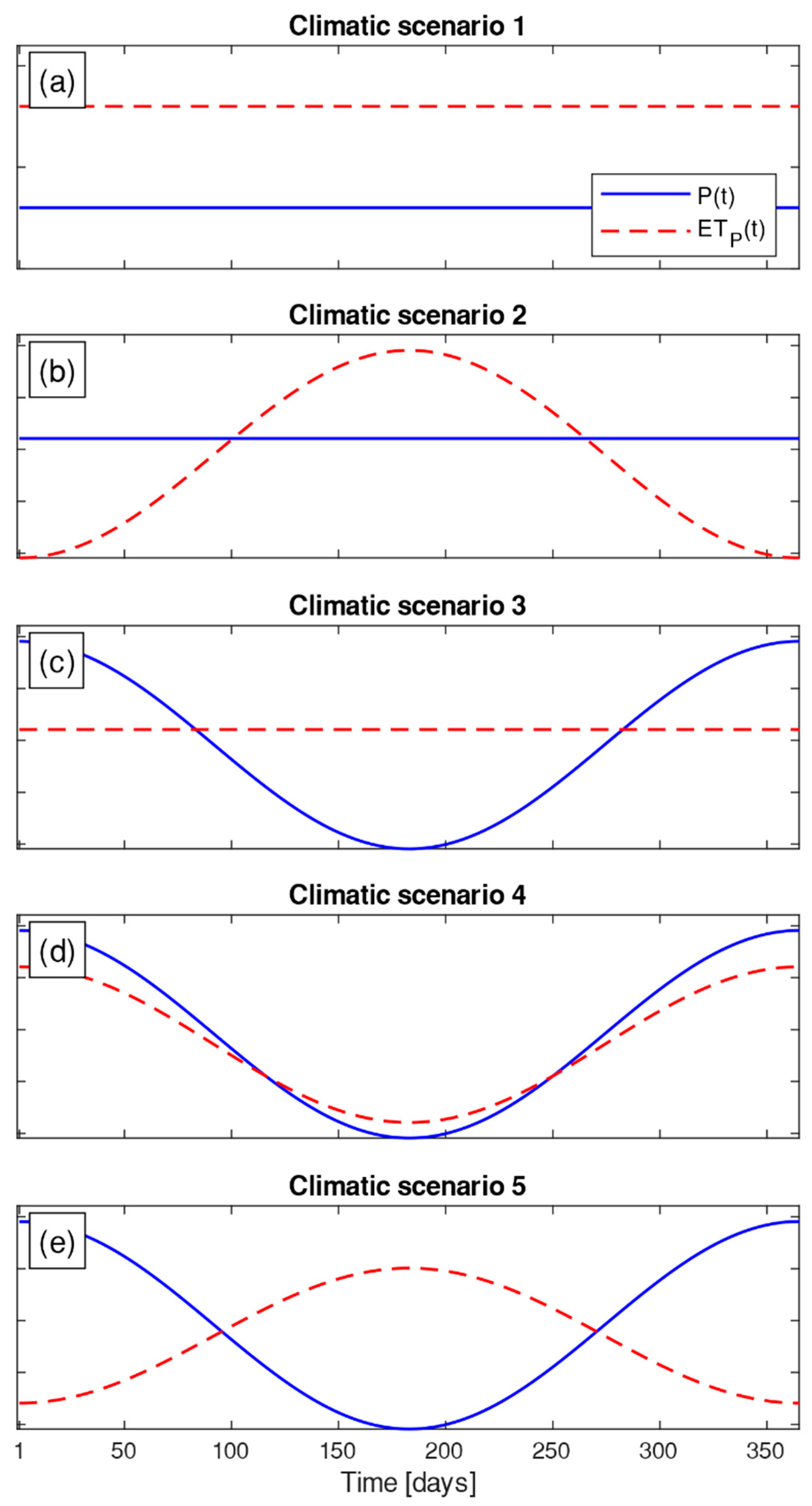
To take into account the role of climate in water partitioning, we considered five climatic scenarios which roughly mimic some of the most frequent climate conditions. As specified before, every climate is characterized here by different seasonal patterns of rain and potential evapotranspiration. Within a given climate, we generated synthetic series of rainfall $P\left(t\right)$ and $E{T}_P\left(t\right)$ at daily time scale $t$ using a weather generator. The five climatic scenarios are intended to represent the seasonal variability of rain and potential evapotranspiration time patterns, as illustrated in Figure 2. The idea of exemplifying climate in such a simple schematization refers to Viola et al. [37], where it has been used to investigate green roof retention performances. The first climatic scenario (Figure 2a) represents stationary condition of rain and potential evapotranspiration during the year. This is an ideal situation in which the variance of meteoclimatic variables is zero, being the less realistic seasonal pattern of the five proposed in this work. The second case (Figure 2b) is typical of oceanic areas with almost constant precipitation during the hydrological year, while potential evapotranspiration has a peak. Climatic scenario 3 (Figure 2c) is the opposite of the last ones, namely potential evapotranspiration is almost constant and major precipitation values are observed during a specific rain season. This climatic scenario is attributable to a tropical climate with high constant temperatures along the year and a monsoon season with a precipitation peak. The feature of climatic scenario 4 (Figure 2d) is in-phase climatic forcing: this is a classic case of humid subtropical climates, where the precipitation peak occurs simultaneously with the temperature one. The last case is the opposite of the climatic scenario 4 (Figure 2e), that is rainfall and potential evapotranspiration are in counter-phase during the hydrological year. Mediterranean climate is well represented by this climatic scenario, because it is well known that rainfall mostly occurs during the winter, while temperature peaks occur in the summer.

In this work the synthetic time series $P\left(t\right)$ and $E{T}_P\left(t\right)$ referring to climatic scenarios were created by the weather generator proposed by Viola, Hellies, and Deidda [37], whose parameters have been calibrated according to main climatic features observed in 10,000 observational sites worldwide. The rain series are intended as daily precipitation arising from a non-stationary and cyclic Poisson point process, characterized by a frequency $1/\lambda \left(t\right)$ (rate of the Poisson process occurrences, (1/days)). The $\lambda \left(t\right)$ parameter was modeled as a sinusoidal function of time $t$ (days), with amplitude $\overline{\lambda }$, the average interarrival time (days) between two rain events and one-year period, as described in in the following equation:

$$\lambda \left(t\right)=\overline{\lambda }\left(1+{\delta }_{\lambda }\sin \left(\frac{2\pi t}{365}+{\omega }_{\lambda }\right)\right),$$

(2)

where ${\delta }_{\lambda }$ characterizes the ratio of the semi-amplitude of the annual harmonics of $\lambda \left(t\right)$ to the annual average, while ${\omega }_{\lambda }$ is the initial phase of the sinusoidal function. Every day with precipitation different to a zero event $P\left(t_i\right)$ (mm/day), where i subscript indicates rain days in the $P\left(t\right)$ series, is simulated as a random process extracted from an exponential distribution with mean daily value $\alpha \left(t\right)$ (mm/day), modeled as follows:

$$\alpha \left(t\right)=\overline{\alpha }\left(1+{\delta }_{\alpha }\sin \left(\frac{2\pi t}{365}+{\omega }_{\alpha }\right)\right),$$

(3)

where $\overline{\alpha }$ is the average amount of rainfall (mm/day), ${\delta }_{\alpha }$ represents the ratio of the semi-amplitudes of the annual harmonics of $\alpha \left(t\right)$ to the annual average, and ${\omega }_{\alpha }$ is the value of phase when $t=0$. Therefore, Equations (1) and (2) allow us to calculate mean interarrival times and mean daily precipitation along the year, which in turns allow us to randomly obtain rain time series.

Similarly, the daily potential evapotranspiration series $E{T}_P\left(t\right)$ (mm/day) are defined as a sinusoidal function with a similar structure to the previous one:

$$E{T}_P\left(t\right)=\overline{E{T}_P}\left(1+{\delta }_E\sin \left(\frac{2\pi t}{365}+{\omega }_E\right)\right),$$

(4)

where $\overline{E{T}_P}$ is the daily mean evapotranspiration (mm/day), ${\delta }_E$ the ratio of the semi-amplitude of the annual harmonics of $E{T}_P\left(t\right)$ to the annual average, and ${\omega }_E$ is the initial phase.

Each climate is defined by a phase between rain and potential evapotranspiration (as described by ${\omega }_{\lambda }$, ${\omega }_{\alpha }$ and ${\omega }_E$) and by a specific seasonal variability of rainfall (as described by ${\delta }_{\alpha }$ and ${\delta }_{\lambda }$) and potential evapotranspiration (modeled by ${\delta }_E$). The values of the semi-amplitude ${\delta }_{\lambda }$, ${\delta }_{\alpha },$ and ${\delta }_E$ have been assessed by Viola, Hellies, and Deidda [37] as the median of their empirical distributions, as observed in 10,000 worldwide stations. For the five climate scenarios, the parameters of the Equations (2)–(4) are reported in

Table 1. Parameters of the sinusoidal Equations (2)–(4) that define the particular pattern of precipitation and potential evapotranspiration, related to the considered climatic scenario. ${\delta }_{\lambda }$, ${\delta }_{\alpha }$ and ${\delta }_E$ represent the ratio of the semi-amplitude of the sinusoidal equations to their mean value, whereas ${\omega }_{\lambda }$, ${\omega }_{\alpha }$, and ${\omega }_E$ are the initial phase. $\overline{\lambda }$, $\overline{\alpha },$ and $\overline{E{T}_P}$ are respectively the average interarrival time, the average amount of daily precipitation, and the average daily potential evapotranspiration.

Climate	$\overline{\mathit{\lambda }}$ (days)	${\mathit{\delta }}_{\mathit{\lambda }}$ (-)	${\mathit{\omega }}_{\mathit{\lambda }}$ (rad)	$\overline{\mathit{\alpha }}$ (mm/day)	${\mathit{\delta }}_{\mathit{\alpha }}$ (-)	${\mathit{\omega }}_{\mathit{\alpha }}$ (rad)	$\overline{\mathit{E}{\mathit{T}}_{\mathit{P}}}$ (mm/day)	${\mathit{\delta }}_{\mathit{E}}$ (-)	${\mathit{\omega }}_{\mathit{E}}$ (rad)
Climatic scenario 1	4.35	0	0	Variable	0	0	Variable	0	0
Climatic scenario 2	4.35	0	0	Variable	0	0	Variable	0.3	−π/2
Climatic scenario 3	4.35	0.45	−π/2	Variable	0.35	π/2	Variable	0	0
Climatic scenario 4	4.35	0.45	−π/2	Variable	0.35	π/2	Variable	0.3	π/2
Climatic scenario 5	4.35	0.45	−π/2	Variable	0.35	π/2	Variable	0.3	−π/2

.

The climate definition, as given above, may embed wide geographic areas where the seasonal patterns of rainfall and potential evapotranspiration are homogeneous, and are described by the six aforementioned parameters. At the same time, annual precipitation and potential evapotranspiration may vary within a climatic area, for instance following topographic gradients. This kind of variability is reflected in the weather generator by allowing us to obtain different aridity indices ($AI$). Numerically, this is achieved by generating synthetic series with different values of $\overline{\alpha }$ and $\overline{E{T}_P}$; we suppose that $\overline{\alpha }$ varies between 3.5–24 (mm/day) and $\overline{E{T}_P}$ between 0.3–5.5 (mm/day). These ranges have been selected considering a realistic range of annual precipitation and potential evapotranspiration. For sake of simplicity, $\overline{\lambda }$ was assumed to be constant, and equal to 4.35 (days) (Table 1) in all the considered climates. This numerical value has been obtained as the mean of the global interarrival times between rainfall events; indeed, the assumption of a unique value restricts the generality of this approach because it hampers the ability to investigate the influence of this parameter on the annual rainfall partitioning, but it is indeed a common and reasonable assumption [20]. Under these conditions, the mean annual amount of precipitation $P$ generated and used in this work can vary between 300 and 2000 mm; similarly, $E{T}_P$ ranges from 100 to 2000 mm.

2.2. EHSM Model

The precipitation $P\left(t\right)$ and the potential evapotranspiration $E{T}_P\left(t\right)$ time series have been then used as an input into a conceptual hydrological model, namely a slight simplified version of the Ecohydrological Streamflow Model (EHSM) [38]. The way the model is used to describe hydrological responses is to represent a basin with two linear reservoirs describing surface and baseflow runoff, and one soil bucket split into two compartments representing the impervious area $c_0$ and the permeable area (1 $-c_0$). The daily precipitation $P\left(t_i\right)$ that falls in the soil bucket is divided in two parts: $c_{0}P\left(t_i\right)$ flows directly in the surface linear reservoir and (1 − $c_0$)$P\left(t_i\right)$ infiltrates in the permeable soil bucket portion (1 − $c_0$) and is accumulated into the soil bucket. Water infiltration and leakage in and from the soil bucket are regulated by 3 parameters: the active soil depth $n{Z}_r$ (mm), which is the product of the soil porosity $n$ (-), the root zone thickness $Z_r$ (mm), the hygroscopic point $s_h$ (-), and the soil moisture at field capacity $s_{fc}$ (-). In order to have only a variable that expresses hydrological soil properties, we condensed $n{Z}_r$, $s_h$, and $s_{fc}$ with the following expression:

$$\zeta =n{Z}_r\left(s_{fc}-s_h\right),$$

(5)

where $\zeta$ (mm) is maximum water holding capacity, representative of maximum amount of water that could be stored in the soil.

The soil moisture of soil bucket regulates the partition of (1 − $c_0$)$P\left(t_i\right)$ in runoff that flows into surface and baseflow linear reservoir. If the soil moisture content exceeds the field capacity, this water volume becomes leakage pulses that feed the linear reservoir which is responsible for baseflow conceptual description. The mean residence time of water within this bucket has been defined as 1/$k_{sub}$ (1/day), which from a physical point of view is related to groundwater dynamics. When soil moisture overpasses saturation, the excess feeds the surface linear reservoir related to surface runoff production. From the union of the outputs of the two linear reservoirs, the model generated the daily runoff series $Q\left(t\right)$.

The model allows us to simulate soil moisture dynamics and the influence of vegetation in drying the soil during two consecutive rain events. In order to quantify the evapotranspiration process, we assumed a limitation induced by the soil moisture that is equal to the maximum value calculated as the product between reference evapotranspiration and the coltural coefficient $K_c$ (-).

The model parameters describing the watershed are only four, summarizing the key processes producing, limiting, and delaying runoff at long time scales. Namely, the selected descriptors are: $\zeta$ maximum water holding capacity, $k_{sub}$ subsurface bucket parameter, $c_0$ impermeable area, and $K_c$ coltural coefficient. For all experiments and demonstrations conducted in this work, the model parameters can vary between physically reasonable ranges, reported in

Table 2. The ranges for the morphological and vegetation parameters used in this work: minimum and maximum supposed values. In the last column, it is stated the value assumed referring to the test-watershed, used for leading our in-silico experiment.

Name	Acronym	Minimum Value	Maximum Value	Test-Watershed
Maximum water holding capacity	$\zeta$ (mm)	18	230	50
Subsurface bucket parameter	$k_{sub}$ (1/day)	0.0017	0.1	0.05
Impervious area	$c_0$ (-)	0	0.05	0.025
Coltural coefficient	$K_c$ (-)	0.5	1.5	1

. It is worth mentioning that $c_0$ range (less than 5%) is reasonable because Budyko’s framework applies to large watersheds, in which impervious surfaces are often spread over the basin. This physically implies that impervious surfaces away from outlet, still contribute to runoff, because the routing drives water volumes to pervious areas, where infiltration occur; this physical process is not accounted in the model. Then, impervious areas in EHSM should be considered as the ones close to the outlet, therefore, we limited the range of $c_0$.

3. Results and Discussions

The simulation outputs are presented in three parts, supporting each of our assumptions: (i) in the first part we show how $\omega$ is unique for a given climate and watershed morphological and vegetation characteristics; (ii) in the second we indicate the effect of climate in water partitioning and (iii) in the last part we quantify the role of basin morphology and vegetation in driving water partitioning for different climate, providing a practical expression of $\omega$.

3.1. Fixed Climate, Fixed Morphology and Vegeatation (FC-FMV)

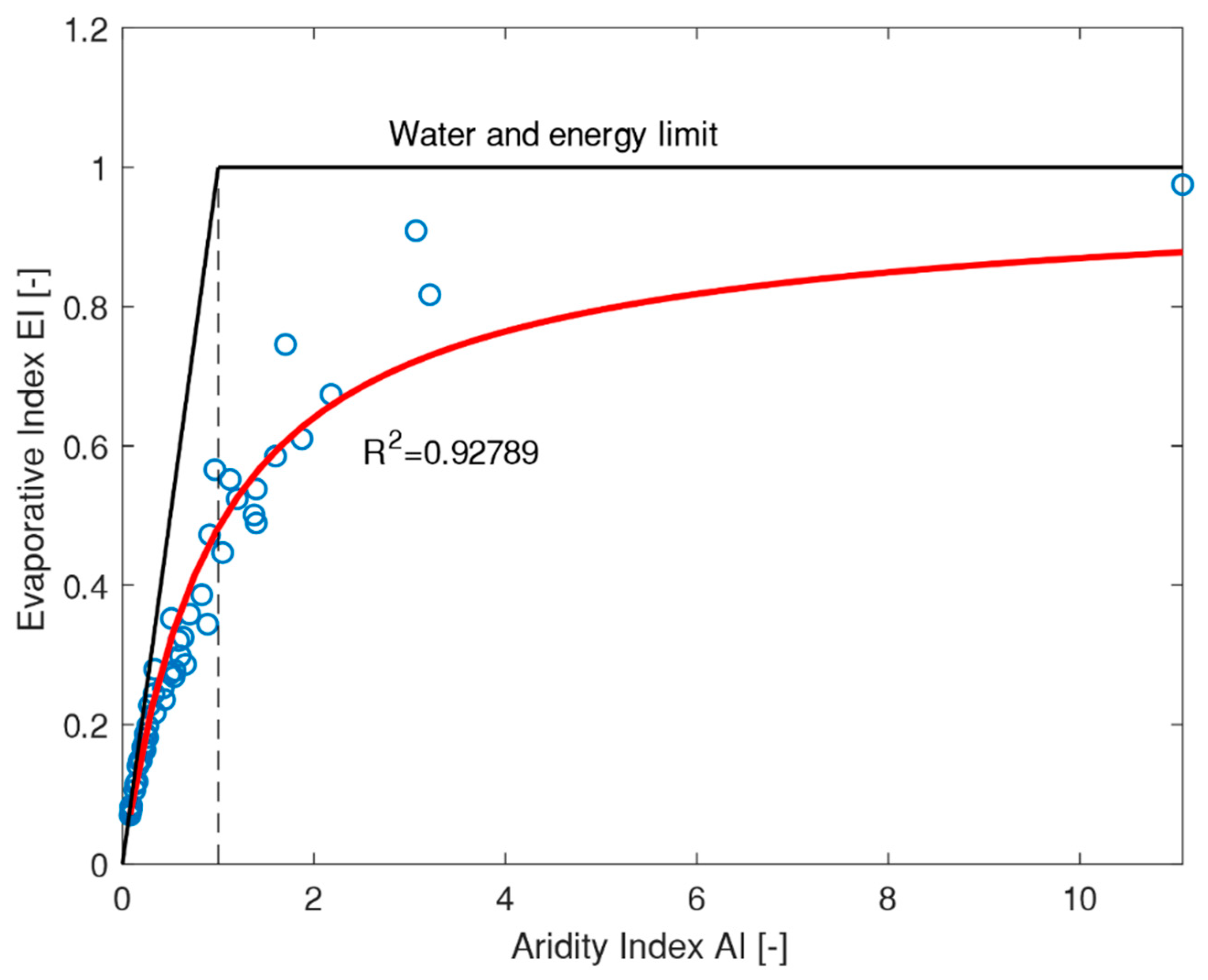
Under a climate scenario and for a given watershed, the first assumption that we aim to prove is the univocity of Fu’s parameter over a wide range of aridity indices (see Figure 1a). Following the method described in Section 2, we generated 50 series of daily precipitation and potential evapotranspiration from a given climatic scenario with a duration equal to 100 years. Every couple of these climatic forcings identified an $AI$’s value. These time series have been used as meteoclimatic input to a test-watershed, in which morphological and vegetation properties are summarized by model parameters reported in the last column in Table 2. Using the model described in Section 2.2 that represented the hydrological response of the test-watershed, we obtained 50 daily time series of runoff $Q\left(t\right)$ and then evapotranspiration series $ET\left(t\right)$, which in turn has been summed at a yearly time scale and then averaged and divided by the related yearly averaged $P$ to obtain 50 values of evaporative index, $EI$. The 50 $AI$-$EI$’s couples may be interpreted as several hydrological responses of the same basin under different aridity index conditions, but under the same climate. The 50 AI-EI’s couples were plotted and the Fu’s equation has been fit to data maximizing the coefficient of determination $R^2$ (Figure 3). After the optimization process, the coefficient of determination $R^2$ obtained was very high for the test-watershed (namely 0.93) meaning that Fu’s equation is a good estimator of water partitioning processes and that the Fu’s parameter could be seen as the hydrological signature of a given basin over different aridity indices within a certain climate. Only few points, with high values of the aridity index, depart from Fu’s curve in Figure 3. This is due to the conceptual model used for describing hydrological processes that allocates a constant percentage of rainfall to surface runoff regardless of the soil and vegetation dynamics under dry conditions (high aridity index values).

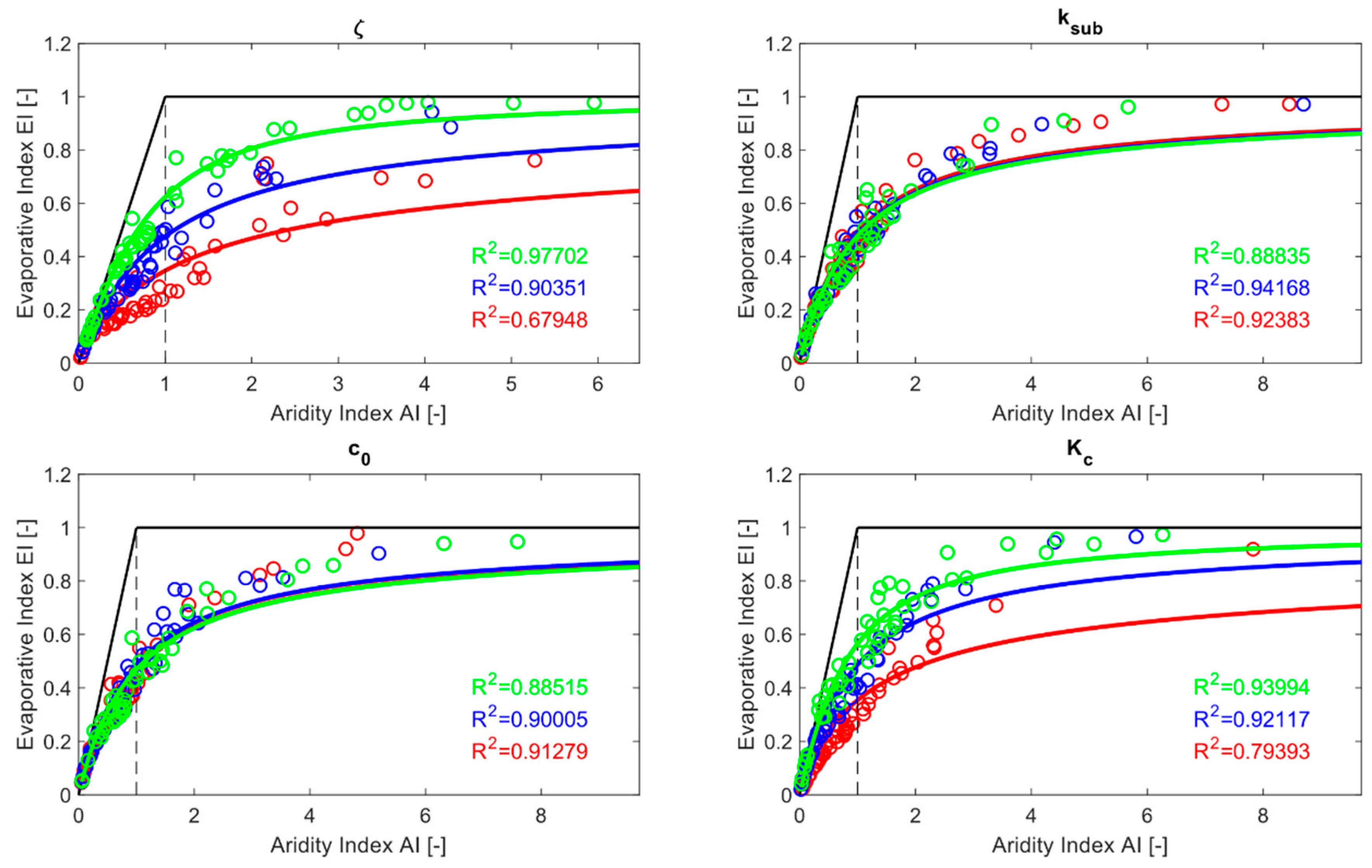
In order to generalize this result, starting from the test-watershed configuration, we tuned morphological and vegetation parameters, once at time, at the minimum/mean/maximum values (reported in Table 2). The number of test-watersheds became nine, for which has been conducted the previous experiment (i.e., the climatic scenario is fixed), in order to demonstrate what has been said in all morphological and vegetation parameter domains. The results are shown in Figure 4, where AI-EI’s couples fit very well to the optimized Fu’s curves, highlighting the generality of the proposed method and the validity of first assumption.

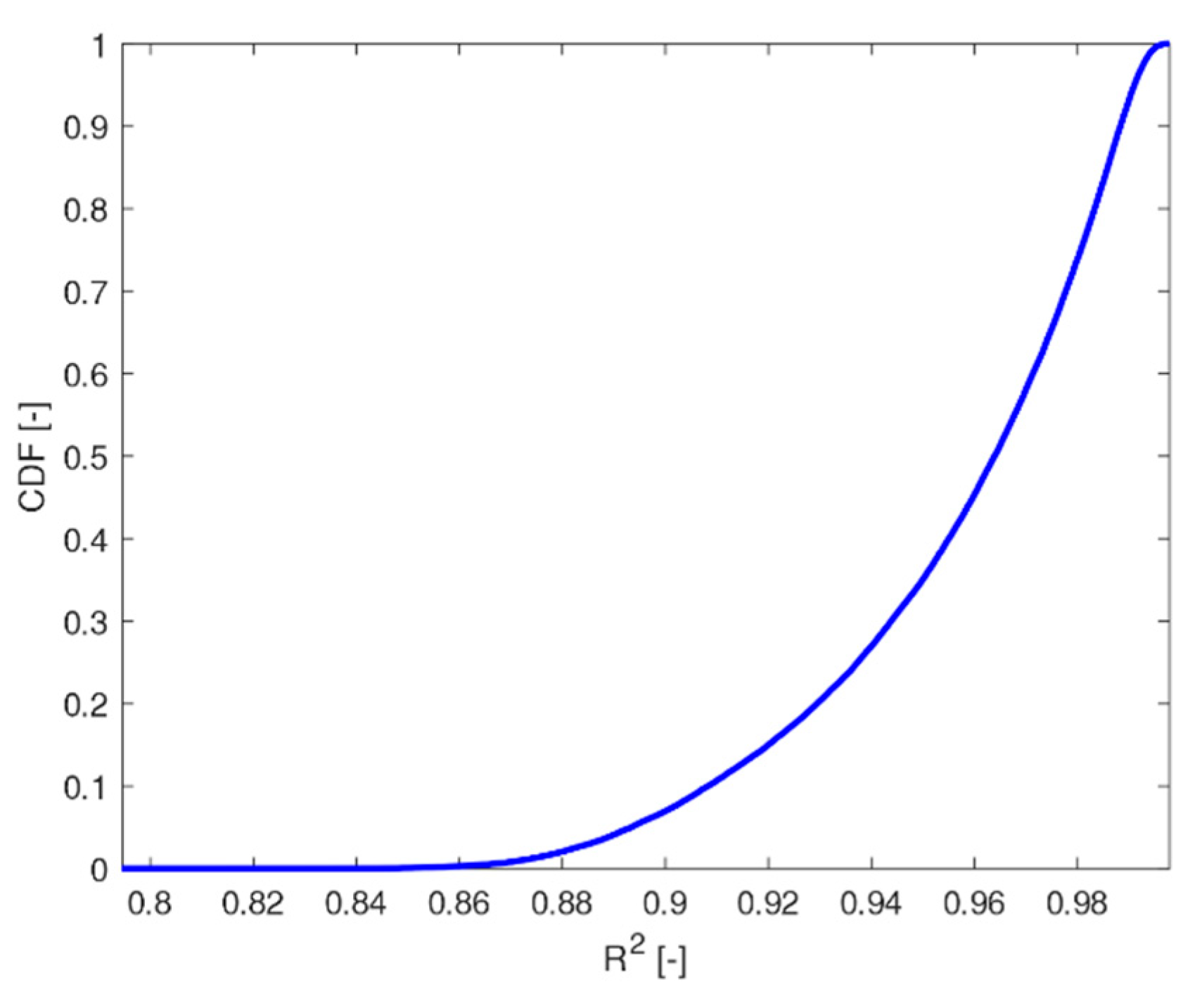
Furthermore and finally, 50,000 combinations of random morphological and vegetation characteristics, extracted from Table 2, and climatic scenarios, were tested to verify that the coefficient of determination is high in every case, regardless of the watershed properties and climate. The number of combination was set to 50,000 for a robust demonstration and in order to limit computational time. Results are presented as the probability distribution of $R^2$, shown in Figure 5. It is easy to note that almost all the examined cases exhibit a high correlation of determination, giving further proof that Fu’s law and $\omega$ are good descriptors of the water partitioning process.

Generally, we can say that, once climate and basin morphological and vegetation properties have been defined, then the hydrological behavior is a function of the aridity index and the long term water partitioning rules can be described with low uncertainties by the Fu’s curve.

3.2. Varying Climate, Fixed Morphology and Vegetation (VC-FMV)

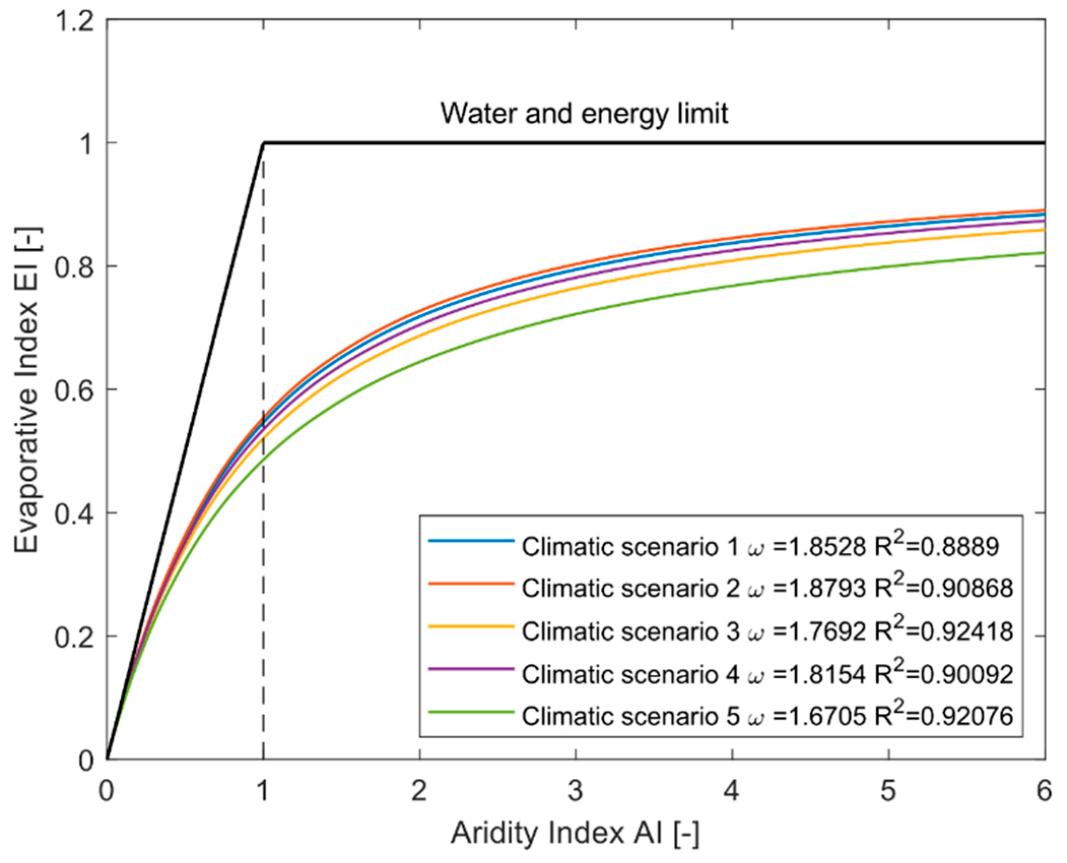
In Section 3.1 we showed that, for a given watershed and climate, only the aridity index drives the rainfall partitioning. Now we explore the influence of climate in water partitioning processes (see Figure 1b). As in the last section, we applied the same methodology recursively involving the test-watershed for the five different climatic scenarios, and we compared the different Fu’s parameters obtained. We basically intended to transpose the test-watershed in different geographic areas (with different climate) and observe the long-time hydrological responses. The five analytical Fu’s curves associated with the five-climatic scenarios and $\omega$ are reported in Figure 6.

In line with what has already been seen in the previous section, for each climate scenario R² has a value close to one, demonstrating that the univocal hydrological response is a condition independent of the climate scenario considered.

Observing the five curves, we can state that climate is an important driver in runoff (and evapotranspiration) generation. The climate seems to define different hydrological behavior for the same watershed, as already pointed out by Budyko [10], Potter, Zhang, Milly, McMahon, and Jakeman [17]. Under climate scenarios 1, 2, and 4, the test-watershed results show less mean annual runoff $Q$ (higher $\omega$ values) than in the 3 and 5 cases. The physical explanation lies in the potential evapotranspiration seasonal pattern: indeed, high evapotranspitative demand during the rain season prevents soil saturation and consequently disadvantages subsurface and surface runoff generation. The climatic scenarios 3 and 5 induce the opposite hydrological behavior due to the aforementioned mechanism. Under these climate conditions, the soil moisture is often equal to the maximum water holding capacity, which implies frequent surface and subsurface runoff production and then higher mean annual runoff $Q$. This happens because in the wettest periods of the year, potential evapotranspiration assumes its minimum value.

Fu’s parameter is strictly correlated to the rain and evapotranspiration seasonal patterns, as demonstrated by Feng et al. [39]. Particularly in climatic scenario 5, characterized by out-of-phase rain and potential evapotranspiration, the $\omega$ value is lower (1.67) while in case 4 involving in-phase rain and potential evapotranspiration, $\omega$ is almost equal to 1.88.

3.3. Varying Climate, Varying Morphology, and Vegetation (VC-VMV)

In this section, we show how basin morphological and vegetation properties are significant in the water partition process (see Figure 1c). To describe such a relation, we proceeded as follows: for all climatic scenarios, we considered 10,000 random watersheds, creating 10,000 independent morphological and vegetation parameter sets, each chosen within the ranges reported in Table 2. By using the procedure described in Section 2 and already used in Section 3, for each morphological and vegetation parameter set, we evaluated the relative Fu’s parameter. The intermediate results are five databases, composed by 10,000 parameter sets and the associated $\omega$ values. To investigate the relationship between hydrological response (represented by $\omega$) and morphological and vegetation descriptors ($\zeta$, $k_{sub}$, $c_0$, $K_c$), we applied stepwise linear regression to mathematically investigate the possible links.

Results of linear regression are reported in

Table 3. Results of the linear regression between morphological and vegetation parameters and Fu’s parameter for all the considered climates. The $a_i$, $\beta$, and $R^2$ respectively represent the coefficients related to each morphological and vegetation parameter, the constant term, and the coefficient of determination of the linear equations that allow obtaining an empirical estimate of $\omega$. All terms of the equation are obtained by stepwise regression, linking the random generated morphological and vegetation parameters’ sets (which value’s range are reported in Table 2) and the associated $\omega$. The colors of the cells are related to the p-value: white cells represent the p-value equal to 0, light grey cells represent p-values higher than 0 and lower than 0.25, and the dark grey cells indicate p-values bigger than 0.25.

Climate	${\mathit{a}}_{\mathit{i}}$				$\mathit{\beta }$	${\mathit{R}}^2$ (-)
	$\mathit{\zeta }$	${\mathit{k}}_{\mathit{s}\mathit{u}\mathit{b}}$	${\mathit{c}}_0$	${\mathit{K}}_{\mathit{C}}$	Intercept
Climatic scenario 1	0.008699	1.207	−5.532	2.623	−0.576	0.784
Climatic scenario 2	0.008379	0.044	−5.853	2.484	−0.385	0.809
Climatic scenario 3	0.005831	−0.179	−5.697	1.979	−0.035	0.867
Climatic scenario 4	0.007851	0.214	−5.939	2.405	−0.393	0.837
Climatic scenario 5	0.003725	0.177	−3.475	1.287	0.516	0.901

for all considered climates, where we reported the $a_i$ coefficient associated with morphological and vegetation parameters, as well as intercept $\beta$ and $R^2$, whereas colors refer to p-values. More precisely, white cells represent a p-value equal to 0, light grey cells represent p-values higher than 0 and lower than 0.25, and dark grey cells indicate p-values bigger than 0.25.

Generally, there is a good correlation between $\omega$ and basin morphological and vegetation descriptors for every climate, which is demonstrated by elevated values of $R^2$. The best result is obtained for climatic scenario 5, where $R^2$ is equal to 0.901. The most significative parameter is $K_c$, the coltural factor (p-values = 0, for all climates). This means that the vegetation plays a significate role in water partitioning processes. In line with the positive sign of the related coefficient/weight (Table 3), $K_c$ is the most important contributor to evapotranspiration. $k_{sub}$, by contrast, does not have a critical role in water partition processes as stated by the related p-value. The subsurface bucket parameter does not appear as a key descriptor of long-term water balance dynamics.

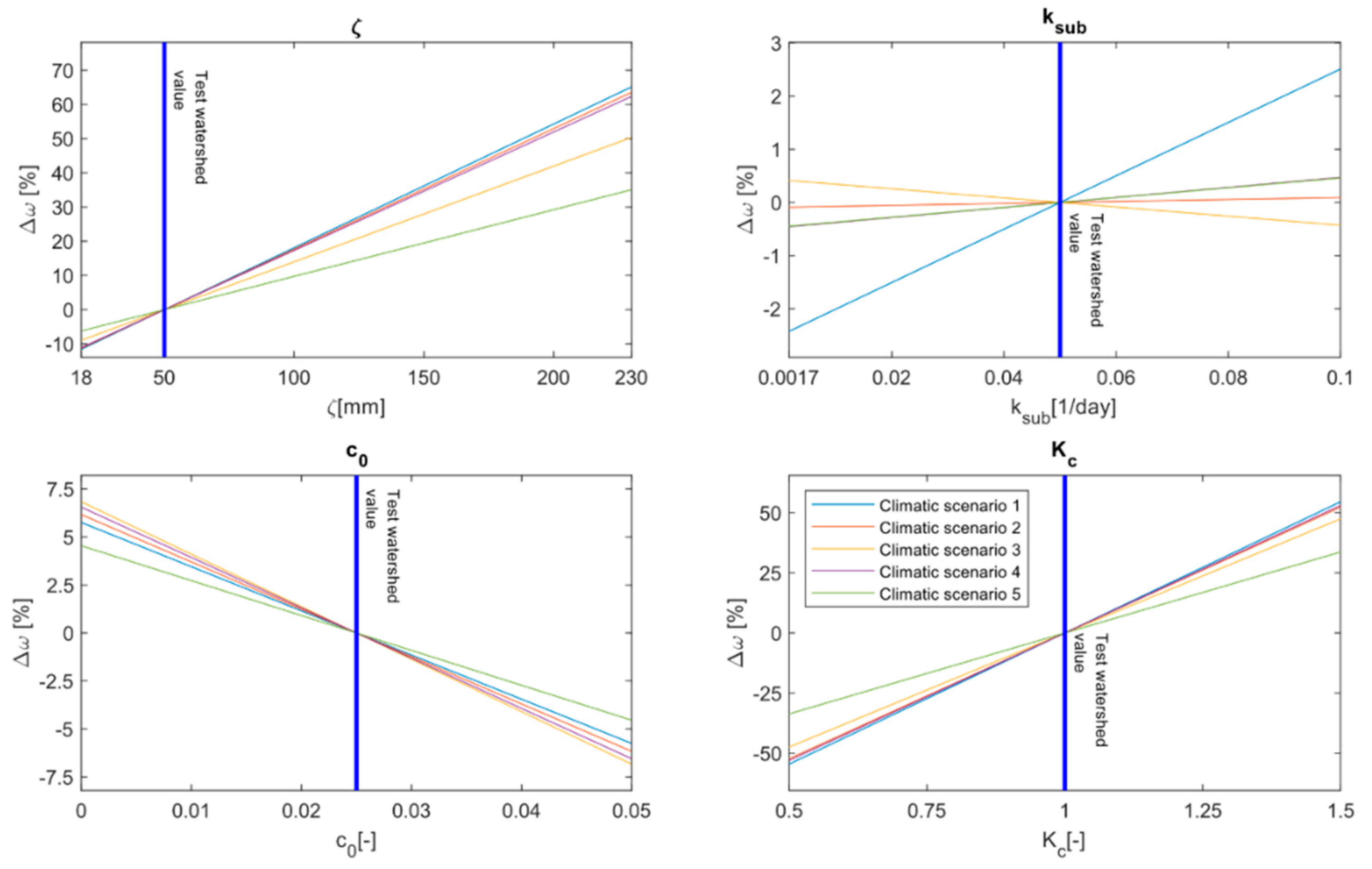
In order to determine the role of each morphological and vegetation descriptor in determining $\omega$, we performed a simple sensitivity analysis (Figure 7). Of course, since the regression equations are linear, results were immediately obtained. Our aim was to represent how the variation of morphometric and vegetation variables affects by the water partitioning process. This analysis is an attempt to represent the influence of the EHSM parameters on $\omega$. Fu’s parameter is particularly sensitive to the coltural coefficient $K_c$: assuming an increasing (decreasing) from the value of the test-watershed to the related extreme, both defined for the coltural coefficient in Table 2, the parameter influences $\omega$ in +26%–+51% (−26%–−51%). Effects on $\omega$ due to an increase (or decrease) of $\zeta$ have the same sign of the latter, but this parameter seems to be less sensitive, as shown by lower slopes of the related sensitivity curves in Figure 7. The effect of vegetation and hydraulic soil capacity is fundamental in the water partitioning processes, and the change of type and quantity can particularly modify the runoff and evapotranspiration’s relative magnitude [6,30,32,40]. The influence of impervious areas $c_0$ is less pronounced than the last two variables, but it plays an important role in hydrological response. The influence of $k_{sub}$ is negligible because subsurface runoff timing has not a fundamental role in long term hydrological processes. In our work we supposed a maximum delay for transformation of subsurface flow in runoff of the order of 600 days ($k_{sub}$ = 1/600 = 0.017). This means that most of the water becomes runoff $Q$ in about two years; this does not influence the water balance during a long-term period and thus it could be considered a constant background noise that does not affect the rules of water partitioning.

Known the effect of different parameters and in order to demonstrate how morphological and vegetation parameters influence runoff, we used the latter results in an additional analysis. We perturbed morphological and vegetation parameters one at the time from the same test-watershed reported in Table 2; then we evaluated ω using the regression equations previously obtained and we evaluated the mean annual runoff alteration $\Delta Q$ due to morphological and vegetation parameter variation for all climatic scenarios. In Figure 8, we represent the influence of parameters on mean annual runoff $Q$ for 10, 20, and 30 per cent positive and negative variations. As each of the considered variables increases or decreases, the figure shows how runoff is modified from the reference condition, as a function of the aridity index. We report results of climatic scenario 5 (the Mediterranean climate) but similar results have been obtained for the other ones considered. For all morphological and vegetation parameters, the pattern of curves is the same and related to the magnitude of $\omega$’s variation. Clearly, moving from low to high $AI$’s values, the magnitude of runoff variation $\Delta Q$ is always raising. This means that, in climate change conditions, as annual rainfall is decreasing and potential evapotranspiration is increasing [41], non-negligible runoff changes are foreseen, leading to important economic and environmental impacts.

The coltural coefficient $K_c$ has a tremendous effect on $\Delta Q$: remarkably, positive or negative variations have not experienced the same impacts. For instance, deforestation or afforestation on the same area induces different runoff changes. Negative alteration of $K_c$ (i.e., deforestation) induces annual runoff to increase more, as a percentage, than the values obtained with positive $K_c$ variations (i.e., afforestation).

4. Case Study Basins

In order to demonstrate the ability of the obtained regression equations to reproduce $\omega$ in different climate in the real world, we used four case study catchments, associated with the last four climatic scenarios considered. The first climatic scenario has been neglected since it is an ideal condition. We compared the values collected from regression equations (in this work called “assessed $\omega$”) with the ones calculated by fitting the Fu’s curve to hydrological data (called “hydrological $\omega$”).

The first case study is Saline River Basin at Rye, Arkansas (USA) and it is a sub-catchment of Ouachita River with an extension of 2102 km². The climate is Atlantic-oceanic with constant precipitation during the year and potential evaporation that has a peak in the summer months (June–August). We observed that its climatic condition is associable with climate scenario 2. Mean annual precipitation $P$ is 1314 mm with a runoff coefficient of 0.33, while mean annual potential evapotranspiration $E{T}_P$ is 945 mm, close to real evapotranspiration $ET$ (883.6 mm). Evergreen forest is the most prevalent land use coverage (96%) and the remaining part is urban and built-up areas.

The second case is the Parana River at Guaira, which is in South America and passes through Brazil, with an approximate area of 830,000 km². The climate is tropical with a constant value of potential evapotranspiration and a precipitation peaks in December, following seasonal pattern of climatic scenario 3. The mean annual precipitation is pretty high (1469.7 mm), as is the mean annual potential evapotranspiration (1368.15 mm); the runoff coefficient is about 0.22, also due to high mean annual evapotranspiration (1144.15 mm). The largest part of the basin is covered by pasture (44%), while annual crop and sugar cane occupy the 27% and 9% of the watershed, respectively; finally, forest is only the 9% of the total of Parana basin.

The third case study is a tributary of the Missouri River and its basin covers three USA states: Montana, North Dakota and South Dakota with a catchment area of 1970 km². to the climate in this area satisfies climate condition 4, with the most important precipitations in the summer months and a mean annual value of 394.2 mm. Precipitation is in-phase with the potential evapotranspiration that has a maximum in the middle of the year, with a mean annual value of 1022 mm. Runoff coefficient is 0.06 and mean annual evapotranspiration is 372.3 mm. The vegetation consists of permanent wetland (61%) and woody savannah (37%).

The latter case study refers to a watershed in California, namely the Santa Ysabel Creek, with a typical Mediterranean climate, characterized by wet winter/autumn and dry summers, attributable to climatic scenario 5. Santa Ysabel Creek has an extension of 112 km², $P$ is 521.95 mm; only a small fraction of rainfall, namely 6%, is transformed into discharge. The mean potential annual evapotranspiration $E{T}_P$ is 1405.25 mm due to high temperature and only 489.1 mm becomes real evapotranspiration $ET$ because of soil moisture limitation. Forest and shrubland are the prevalent land cover type (51% and 46%), with a small amount of savannas.

Monthly rainfall and temperature in the four considered case study are represented in Figure 9. Climatic data are provided by different sources: for the three US watersheds (Saline River Basin at Rye, the tributary of the Missouri River and Santa Ysabel Creek) we used the Model Parameter Estimation Experiment (MOPEX) [35], while for the Parana at Guaira basin we employed CRU TS version 4.00 [42], the CGIAR-CSI Global Aridity Index (Global-Aridity), and the Global Potential Evapo-Transpiration (Global-PET) Climate Database [43,44]. In order to give a morphological and vegetation characterization of the study cases, different sources of data have been used: for the three US watersheds, the MOPEX [35] database was used, and for Parana at Guaira basin, the info reported by Melo et al. [45] and soil maps were utilized.

Starting from the basin morphological and vegetation characteristics, we calculated the four aforementioned model parameters ($\zeta$, $k_{sub}$, $c_0,$ and $K_c$). The maximum water holding capacity $\zeta$ was calculated using different soil parameters, according to Equation (5). $n$, $s_{fc}$ and $s_h$ were obtained from soil type information, while $Z_r$ was related to the vegetation type within the considered basin following Yang et al. [46]. The evaluation of the subsurface parameter $k_{sub}$ was done using the global maps provided by Beck et al. [47]. The percentage of impervious area $c_0$ was obtained from soil use information reported within the mentioned database. The coltural coefficient $K_c$ was presumed to be related to vegetation type; we set a value of 1.5 for forest, 1.25 for shrubland and savannahs, 1 for cropland and grassland, and 0.5 for bare soil. Then, a weighted average provided a unique value over the considered basins.

Once we had calculated the model parameters, we then calculated $\omega$ through the regression equations of Section 3.3 and reported values in the column “Assessed $\omega$” in

Table 4. Case study basins, their associated climatic scenario, and morphological and vegetation parameters, evaluated by a “general database”, composed by the MOPEX database [35], Padrón, et al. [48], Melo, Scanlon, Zhang, Wendland and Yin [45], and other mixed information. The last three columns point out the results of comparison between “hydrological $\omega$” (obtained by the Fu’s expression) and “assessed $\omega$” (obtained by the proposed regression equations).

Case Study	Climatic Scenario	$\mathit{\zeta }$ (mm)	${\mathit{k}}_{\mathit{s}\mathit{u}\mathit{b}}$ (1/day)	${\mathit{c}}_0$ (-)	${\mathit{K}}_{\mathit{c}}$ (-)	Hydrologic $\mathit{\omega }$	Assessed $\mathit{\omega }$	$\Delta \mathit{\omega }$ (%)
Saline River near Rye	2	155.05	0.08	0.03	1.50	4.50	4.44	1.21%
Parana River at Guaira	3	146.95	0.08	0.02	1.13	2.96	2.92	1.25%
Little Missouri at Camp Crook	4	44.41	0.17	0.01	1.25	2.92	2.90	0.60%
Santa Ysabel Creek near Ramona	5	96.35	0.09	0.00	1.38	2.72	2.63	3.10%

. On the other hand, climatic and hydrological data also allowed us to define $AI$ and $EI$ for each case study, and consequently $\omega$ could be assessed by making the Fu’s curve pass through those points. A simple comparison has been carried out between the “hydrological” and “assessed” $\omega$ values, while the relative percentual difference $\Delta \omega$ was assessed and reported in Table 4. For the considered case study, errors are indeed limited, with only 3% for the Santa Ysabel Creek near Ramona.

The results are encouraging, but it is necessary to underline some limitations of the proposed method. First, the definition of a climatic pattern may be too simplistic in representing seasonal behavior of rainfall and potential evapotranspiration worldwide. In addition, the daily rainfall representation as a Poissonian process, with a constant interarrival time, could result in errors in streamflow estimation. In fact low values of $\overline{\lambda }$ imply elevate soil moisture and more runoff production and vice versa. Thus, a correct characterization of $\overline{\lambda }$ is crucial for a precise description of long-term hydrological dynamics.

5. Conclusions

In this work, we examined the complex relations between climatic, morphological, and vegetation watershed properties and long term water partitioning processes. We provided simple equations for calculating the Fu’s parameter $\omega$ in hydrological data poor conditions. We believe that the proposed tool will help practitioners and hydrologists to assess mean annual runoff, even in ungauged basins.

We used five seasonal patterns of precipitation and potential evapotranspiration and chose four basin morphological and vegetation descriptors ($\zeta$, $k_{sub}$, $c_0$ and $K_c$) to summarize climate and basin characteristics. First, given a climate and a basin, we demonstrated that water partitioning is only related to the aridity index, which is a measure of local climatic conditions. This was based on a different point of view about Budyko’s theory: water partitioning rules for a given basin, in a given climatic scenario, forced by different couples of stochastic $P\left(t\right)$ and $E{T}_P\left(t\right)$, are well described by a Fu’s curve, as stated by the high values of coefficient of determination $R^2$ (Figure 3, Figure 4 and Figure 5).

Second, we conducted an experiment to assess the climate effect in determining $\omega$; we simulated hydrological behavior of the same watershed within different climatic scenarios. As expected, water partition is heavily affected by climate: under a Mediterranean climate we observed the highest mean annual runoff Q, while the oceanic climate was the driest among the considered climatic scenarios. This means that seasonal patterns and the phase between precipitation and potential evapotranspiration (temperature) play a non-negligible role in long term water partitioning.

Third, we evaluated how the morphological and vegetation properties influence water partitioning. Then, given different climate and different watersheds, we mathematically described the effect of morphological and vegetation descriptors in water partitioning processes. Five linear regressions between the four model parameters and $\omega$ have been calculated, one for each climatic scenario. We showed that the coltural coefficient $K_c$ and the maximum soil water holding capacity $\zeta$ are the most important factors in influencing long term hydrological processes. Finally, we tested the linear regressions performances in four case studies in the US and South America, and obtained encouraging results.

Obviously, the range within which regression equations have been tuned (Table 2) and the limited number of parameters (Section 2.2) are a limitation for the presented method, which introduces further approximation within Budyko’s theory. Nevertheless, the regression equations enlarge the feasibility of Fu’s equation, providing a rough assessment of annual runoff in limited data conditions and with low computational effort.

References

- Vörösmarty, C.J.; Green, P.; Salisbury, J.; Lammers, R.B. Global water resources: vulnerability from climate change and population growth. Science 2000, 289, 284–288. [Google Scholar] [CrossRef] [PubMed]
- Abatzoglou, J.T.; Ficklin, D.L. Climatic and physiographic controls of spatial variability in surface water balance over the contiguous United States using the Budyko relationship. Water Resour. Res. 2017, 53, 7630–7643. [Google Scholar] [CrossRef]
- Schaake, J.C.; Koren, V.I.; Duan, Q.Y.; Mitchell, K.; Chen, F. Simple water balance model for estimating runoff at different spatial and temporal scales. J. Geophys. Res. Atmos. 1996, 101, 7461–7475. [Google Scholar] [CrossRef]
- McCabe, G.J.; Wolock, D.M. Independent effects of temperature and precipitation on modeled runoff in the conterminous United States. Water Resour. Res. 2011, 47. [Google Scholar] [CrossRef]
- Porporato, A.; Daly, E.; Rodriguez-Iturbe, I. Soil water balance and ecosystem response to climate change. Am. Nat. 2004, 164, 625–632. [Google Scholar] [CrossRef]
- Donohue, R.J.; Roderick, M.L.; McVicar, T.R. On the importance of including vegetation dynamics in Budyko’s hydrological model. Hydrol. Earth Syst. Sci. 2007, 11, 983–995. [Google Scholar] [CrossRef]
- Koster, R.D.; Suarez, M.J. A simple framework for examining the interannual variability of land surface moisture fluxes. J. Clim. 1999, 12, 1911–1917. [Google Scholar] [CrossRef]
- Shao, Q.; Traylen, A.; Zhang, L. Nonparametric method for estimating the effects of climatic and catchment characteristics on mean annual evapotranspiration. Water Resour. Res. 2012, 48. [Google Scholar] [CrossRef]
- Zhang, L.; Hickel, K.; Dawes, W.R.; Chiew, F.H.S.; Western, A.W.; Briggs, P.R. A rational function approach for estimating mean annual evapotranspiration. Water Resour. Res. 2004, 40, W025021–W02502114. [Google Scholar] [CrossRef]
- Budyko, M. Climate and Life; Academic Press: New York, NY, USA, 1974; p. 508. [Google Scholar]
- Wang, C.; Wang, S.; Fu, B.; Zhang, L. Advances in hydrological modelling with the Budyko framework: A review. Prog. Phys. Geogr. 2015, 40, 409–430. [Google Scholar] [CrossRef]
- Zhang, L.; Dawes, W.R.; Walker, G.R. Response of mean annual evapotranspiration to vegetation changes at catchment scale. Water Resour. Res. 2001, 37, 701–708. [Google Scholar] [CrossRef]
- Budyko, M. The Heat Balance of the Earth’s Surface. Available online: https://www.cia.gov/library/readingroom/docs/CIA-RDP81-01043R002500010003-6.pdf (accessed on 5 November 2019).
- Donohue, R.J.; Roderick, M.L.; McVicar, T.R. Roots, storms and soil pores: Incorporating key ecohydrological processes into Budyko’s hydrological model. J. Hydrol. 2012, 436–437, 35–50. [Google Scholar] [CrossRef]
- Gerrits, A.M.J.; Savenije, H.H.G.; Veling, E.J.M.; Pfister, L. Analytical derivation of the Budyko curve based on rainfall characteristics and a simple evaporation model. Water Resour. Res. 2009, 45. [Google Scholar] [CrossRef]
- Feng, X.; Vico, G.; Porporato, A. On the effects of seasonality on soil water balance and plant growth. Water Resour. Res. 2012, 48. [Google Scholar] [CrossRef]
- Potter, N.; Zhang, L.; Milly, P.; McMahon, T.A.; Jakeman, A. Effects of rainfall seasonality and soil moisture capacity on mean annual water balance for Australian catchments. Water Resour. Res. 2005, 41. [Google Scholar] [CrossRef] [Green Version]
- Milly, P. Climate, soil water storage, and the average annual water balance. Water Resour. Res. 1994, 30, 2143–2156. [Google Scholar] [CrossRef]
- Yang, D.; Sun, F.; Liu, Z.; Cong, Z.; Lei, Z. Interpreting the complementary relationship in non-humid environments based on the Budyko and Penman hypotheses. Geophys. Res. Lett. 2006, 33. [Google Scholar] [CrossRef]
- Yokoo, Y.; Sivapalan, M.; Oki, T. Investigating the roles of climate seasonality and landscape characteristics on mean annual and monthly water balances. J. Hydrol. 2008, 357, 255–269. [Google Scholar] [CrossRef]
- Donohue, R.J.; Roderick, M.L.; McVicar, T.R. Can dynamic vegetation information improve the accuracy of Budyko’s hydrological model? J. Hydrol. 2010, 390, 23–34. [Google Scholar] [CrossRef]
- Gentine, P.; D’Odorico, P.; Lintner, B.R.; Sivandran, G.; Salvucci, G. Interdependence of climate, soil, and vegetation as constrained by the Budyko curve. Geophys. Res. Lett. 2012, 39. [Google Scholar] [CrossRef] [Green Version]
- Choudhury, B. Evaluation of an empirical equation for annual evaporation using field observations and results from a biophysical model. J. Hydrol. 1999, 216, 99–110. [Google Scholar] [CrossRef]
- Schreiber, P. Über die Beziehungen zwischen dem Niederschlag und der Wasserführung der Flüsse in Mitteleuropa. Z. Meteorol. 1904, 21, 441–452. [Google Scholar]
- Pike, J. The estimation of annual run-off from meteorological data in a tropical climate. J. Hydrol. 1964, 2, 116–123. [Google Scholar] [CrossRef]
- Turc, L. Le bilan d’eau des sols: relations entre les précipitations, l’évaporation et l’écoulement. Annales Agron. 1954, 5, 491–569. [Google Scholar]
- Ol’Dekop, E. Ob isparenii s poverknosti rechnykh basseinov (On evaporation from the surface of river basins). Trans. on Meteorol. Obs., Univ. Tartu 1911, 4, 200. [Google Scholar]
- Fu, B. On the calculation of the evaporation from land surface. Sci. Atmos. Sin. 1981, 5, 23–31. [Google Scholar]
- Donohue, R.J.; Roderick, M.L.; McVicar, T.R. Assessing the differences in sensitivities of runoff to changes in climatic conditions across a large basin. J. Hydrol. 2011, 406, 234–244. [Google Scholar] [CrossRef]
- Li, D.; Pan, M.; Cong, Z.; Zhang, L.; Wood, E. Vegetation control on water and energy balance within the Budyko framework. Water Resour. Res. 2013, 49, 969–976. [Google Scholar] [CrossRef]
- Williams, C.A.; Reichstein, M.; Buchmann, N.; Baldocchi, D.; Beer, C.; Schwalm, C.; Wohlfahrt, G.; Hasler, N.; Bernhofer, C.; Foken, T.; et al. Climate and vegetation controls on the surface water balance: Synthesis of evapotranspiration measured across a global network of flux towers. Water Resour. Res. 2012, 48. [Google Scholar] [CrossRef]
- Zhang, S.; Yang, H.; Yang, D.; Jayawardena, A.W. Quantifying the effect of vegetation change on the regional water balance within the Budyko framework. Geophys. Res. Lett. 2016, 43, 1140–1148. [Google Scholar] [CrossRef]
- Zhou, G.; Wei, X.; Chen, X.; Zhou, P.; Liu, X.; Xiao, Y.; Sun, G.; Scott, D.F.; Zhou, S.; Han, L.; et al. Global pattern for the effect of climate and land cover on water yield. Nat. Commun. 2015, 6. [Google Scholar] [CrossRef]
- Xu, X.; Liu, W.; Scanlon, B.R.; Zhang, L.; Pan, M. Local and global factors controlling water-energy balances within the Budyko framework. Geophys. Res. Lett. 2013, 40, 6123–6129. [Google Scholar] [CrossRef]
- Duan, Q.; Schaake, J.; Andréassian, V.; Franks, S.; Goteti, G.; Gupta, H.V.; Gusev, Y.M.; Habets, F.; Hall, A.; Hay, L.; et al. Model Parameter Estimation Experiment (MOPEX): An overview of science strategy and major results from the second and third workshops. J. Hydrol. 2006, 320, 3–17. [Google Scholar] [CrossRef] [Green Version]
- Yang, D.; Sun, F.; Liu, Z.; Cong, Z.; Ni, G.; Lei, Z. Analyzing spatial and temporal variability of annual water-energy balance in nonhumid regions of China using the Budyko hypothesis. Water Resour. Res. 2007, 43, 12–16. [Google Scholar] [CrossRef]
- Viola, F.; Hellies, M.; Deidda, R. Retention performance of green roofs in representative climates worldwide. J. Hydrol. 2017, 553, 763–772. [Google Scholar] [CrossRef] [Green Version]
- Viola, F.; Pumo, D.; Noto, L.V. EHSM: A conceptual ecohydrological model for daily streamflow simulation. Hydrol. Process. 2014, 28, 3361–3372. [Google Scholar] [CrossRef]
- Feng, X.; Porporato, A.; Rodriguez-Iturbe, I. Stochastic soil water balance under seasonal climates. Proc. R. Soc. A Math. Phys. Eng. Sci. 2015, 471. [Google Scholar] [CrossRef]
- Wigmosta, M.S.; Vail, L.W.; Lettenmaier, D.P. A distributed hydrology-vegetation model for complex terrain. Water Resour. Res. 1994, 30, 1665–1679. [Google Scholar] [CrossRef]
- Viola, F.; Francipane, A.; Caracciolo, D.; Pumo, D.; La Loggia, G.; Noto, L.V. Co-evolution of hydrological components under climate change scenarios in the Mediterranean area. Sci. Total Environ. 2016, 544, 515–524. [Google Scholar] [CrossRef]
- Harris, I.; Jones, P.D.; Osborn, T.J.; Lister, D.H. Updated high-resolution grids of monthly climatic observations—the CRU TS3.10 Dataset. Int. J. Climatol. 2014, 34, 623–642. [Google Scholar] [CrossRef]
- Trabucco, A.; Zomer, R.J.; Bossio, D.A.; van Straaten, O.; Verchot, L.V. Climate change mitigation through afforestation/reforestation: A global analysis of hydrologic impacts with four case studies. Agric. Ecosyst. Environ. 2008, 126, 81–97. [Google Scholar] [CrossRef]
- Zomer, R.J.; Trabucco, A.; Bossio, D.A.; Verchot, L.V. Climate change mitigation: A spatial analysis of global land suitability for clean development mechanism afforestation and reforestation. Agric. Ecosyst. Environ. 2008, 126, 67–80. [Google Scholar] [CrossRef]
- Melo, D.D.C.D.; Scanlon, B.R.; Zhang, Z.; Wendland, E.; Yin, L. Reservoir storage and hydrologic responses to droughts in the Paraná River basin, south-eastern Brazil. Hydrol. Earth Syst. Sci. 2016, 20, 4673–4688. [Google Scholar] [CrossRef]
- Yang, Y.; Donohue, R.J.; McVicar, T.R. Global estimation of effective plant rooting depth: Implications for hydrological modeling. Water Resour. Res. 2016, 52, 8260–8276. [Google Scholar] [CrossRef] [Green Version]
- Beck, H.E.; van Dijk, A.I.J.M.; Miralles, D.G.; de Jeu, R.A.M.; Bruijnzeel, L.A.; McVicar, T.R.; Schellekens, J. Global patterns in base flow index and recession based on streamflow observations from 3394 catchments. Water Resour. Res. 2013, 49, 7843–7863. [Google Scholar] [CrossRef] [Green Version]
- Padrón, R.S.; Gudmundsson, L.; Greve, P.; Seneviratne, S.I. Large-Scale Controls of the Surface Water Balance Over Land: Insights from a Systematic Review and Meta-Analysis. Water Resour. Res. 2017, 53, 9659–9678. [Google Scholar] [CrossRef]
Figure 1.
(a) Fixed climate, fixed morphology and vegetation: given a climate, a watershed, over different annual precipitation, and potential evapotranspiration, hydrological response follows the same law. (b) Varying climate, fixed morphology and vegetation: given a watershed, the climate drives the hydrological response in different ways. (c) Varying climate, varying morphology and vegetation: for each climate, the water partitioning process is driven by morphological and vegetation properties of the basin.
Figure 2.
Schematic representation of seasonal time patterns of precipitation and potential evapotranspiration. Lines represent the daily mean of stochastic time series, as generated by Equations (2) and (3) for and by Equation (4) as regard to . Parameters are given in Table 1. Following Viola, Hellies, and Deidda [37].
Figure 3.
-’s couples into the Budyko’s domain generated by the combination of weather generator and conceptual model EHSM, the optimised Fu’s curve, and the related coefficient of determination value for the climatic scenario 5 and the test-watershed (see Table 2).
Figure 4.
Fu’s curves obtained considering the test-watershed parameters (blue line, Table 2, last column) and perturbating one parameter at time (one for each panel), testing their minimum (red line, Table 2 second column) and maximum values (green line, Table 2 third column). has been reported for the associated curves.
Figure 5.
Cumulative distribution frequency of of a sample of 50,000 random generated basins. The coefficient of determination describes the goodness of Fu’s equation in describing water partitioning over wide range of aridity indices.
Figure 6.
The five associated Fu’s equations related to the test-watershed in the five different climatic scenarios. In the inset, the optimized and the are reported referring to the five curves.
Figure 7.
Sensitivity analysis on morphological and vegetation regression equations relating model parameters to , in different climates. Coefficients are reported in Table 3. The percentual alteration due to variation of each morphological and vegetation descriptors (ranging between minimum and maximum values reported in Table 2) from the configuration of test-watershed setting, is reported.
Figure 8.
Runoff alteration, under different , referring to the climatic scenario 5 and supposing an increment/decrement of 10, 20, or 30 per cent of the four morphological and vegetation descriptors from the test-watershed configuration. The curves associated with positive alteration of the morphology and vegetation parameters are reported in green and the ones associated with negative variation are in red.
Figure 9.
Seasonal patterns of monthly rainfall and potential evapotranspiration in the four considered case study basins. The red line represents the mean monthly potential evapotranspiration, whereas the blue bar represents the mean monthly precipitations from MOPEX database [35]. For the case study with an asterisk: the precipitation and potential evapotranspiration datasets respectively come from CRU TS version 4.00 [42], the CGIAR-CSI Global Aridity Index (Global-Aridity), and the Global Potential Evapo-Transpiration (Global-PET) Climate Database [43,44].