Characterization of the Groundwater Storage Systems of South-Central Chile: An Approach Based on Recession Flow Analysis


1
Department of Water Resources, Universidad de Concepción, Chillán 3812120, Chile
2
Centro Fondap CRHIAM, Concepción 4070411, Chile
3
Department of Civil Engineering, Universidad Católica de la Santísima Concepción 4090541, Chile
4
Centro de Investigación en Biodiversidad y Ambientes Sustentables CIBAS, Concepción 4090541, Chile
*
Author to whom correspondence should be addressed.
Water 2019, 11(11), 2324; https://doi.org/10.3390/w11112324
Submission received: 16 September 2019
/
Revised: 22 October 2019
/
Accepted: 1 November 2019
/
Published: 7 November 2019
(This article belongs to the Section Hydrology)
Abstract
:Groundwater storage and discharge are important processes that have not yet been sufficiently studied in some parts of Chile. Additionally, in watersheds without snow cover or glaciers, groundwater storage and release are the main sources of minimum flow generation; therefore, improvements are required to characterize this process. This study aimed to use recession flow analysis to link groundwater storage depletion to the predominant geological characteristics of each watershed in order to improve our understanding of the groundwater storage-release process in 24 watersheds in south-central Chile. The results allowed different groundwater storage behaviors associated with different geological characteristics to be identified, making recession flow analysis a valuable tool for improving the representation and conceptualization of this process in order to advance toward better minimum flow predictions.
1. Introduction
Mountain watersheds tend to be dominated by snowmelt or occasionally glacier melt, which are often the main sources of water in adjacent low-lying areas [1]. However, in watersheds without snow cover or glaciers, groundwater storage and release make up the main source of minimum flow (or baseflow) generation, making it an important process in the hydrological system of a watershed [2], and its contribution to river streamflows proves fundamental to meeting the water demands of various economic activities in periods of water scarcity. Therefore, improvements are necessary to characterize the low-flow behavior of rivers for the joint management of water use, water quality management, and ecosystem services [3].
The descending flow of rivers in rainless periods is known as the recession flow. These flows are directly related to the groundwater storage of the watershed; therefore, the groundwater storage and discharge process can be studied through flow measurements during the recession period [4]. Brutsaert and Nieber [5], using recession-period flow data, proposed an analysis method (the recession flow analysis method) to indirectly estimate watershed-scale hydraulic parameters [6] based on the Boussinesq equation, which describes the drainage process of an ideal aquifer. Put simply, the analysis consists of plotting the average recession flow discharge (Q) as a function of the rate of change in discharge (dQ/dt) in log-log space. This allows different recession events to be identified, producing a data cloud that permits different recession regimes to be identified in order to indirectly obtain the hydraulic parameters of the aquifer [6]. However, recent literature has shown that the method can be applied more broadly [7]. For example, Brutsaert [8] showed that flow records can be used to characterize groundwater storage and release processes in a watershed. The author developed a methodology to quantify the variability of long-term groundwater storage using recession flows. Kirchner [9], using the recession flow method, developed a methodology to quantify dynamic groundwater storage, with which the watershed can be represented as a simple dynamic system. The methodology described by the author allows estimates of the dynamic storage of the basin and recession times to be obtained. Ajami et al. [10] used recession flow analysis in the Sabino Creek catchment (United States), which has a fractured rock influence, to derive groundwater storage-release relationships in order to estimate changes in storage to quantify mountain block recharge (MBR) rates. Shaw and Riha [7] applied the recession analysis approach of [5] considering individual events in seven basins in the United States. The authors suggest that individual analysis of recession events can be a valuable tool to obtain information on watershed-scale hydrological processes and can justify alternatives to current low-flow models. According to the literature cited, recession flow data contain information on the dynamic behavior of groundwater storage and release [8,9,10]; thus, these data can represent the rate at which the groundwater storage is depleting (groundwater storage behaviors) and in turn different storage structures. Therefore, the behavior of recession flow data can be associated with the predominant geological characteristics of watersheds to provide a better understanding of hydrological processes in order to improve the structure of hydrological models.
There are various mountain watersheds in Chile with fractured geology (e.g., the watershed system associated with the Chillán volcanic complex), [11,12,13], as well as mountain watersheds with mixed geology [14]. In addition, due to the formation of the country, the Central Valley presents a higher proportion of geological sequences of sedimentary origin [14]; therefore, the watersheds located in this area and mountain watersheds should present different storage behaviors. Thus, the objective of this study is to identify and characterize the behavior of groundwater storage systems in watersheds with different geological characteristics using recession flow analysis to improve our understanding of the groundwater storage-release process.
2. Methods
To study the groundwater storage behavior in the watersheds the recession flow analysis method described in Brutsaert and Nieber [5] was used. Then, to complement the analysis the identified behaviors were linked to the geological characteristics of each watershed.
2.1. Study Area and Hydrometeorological Data
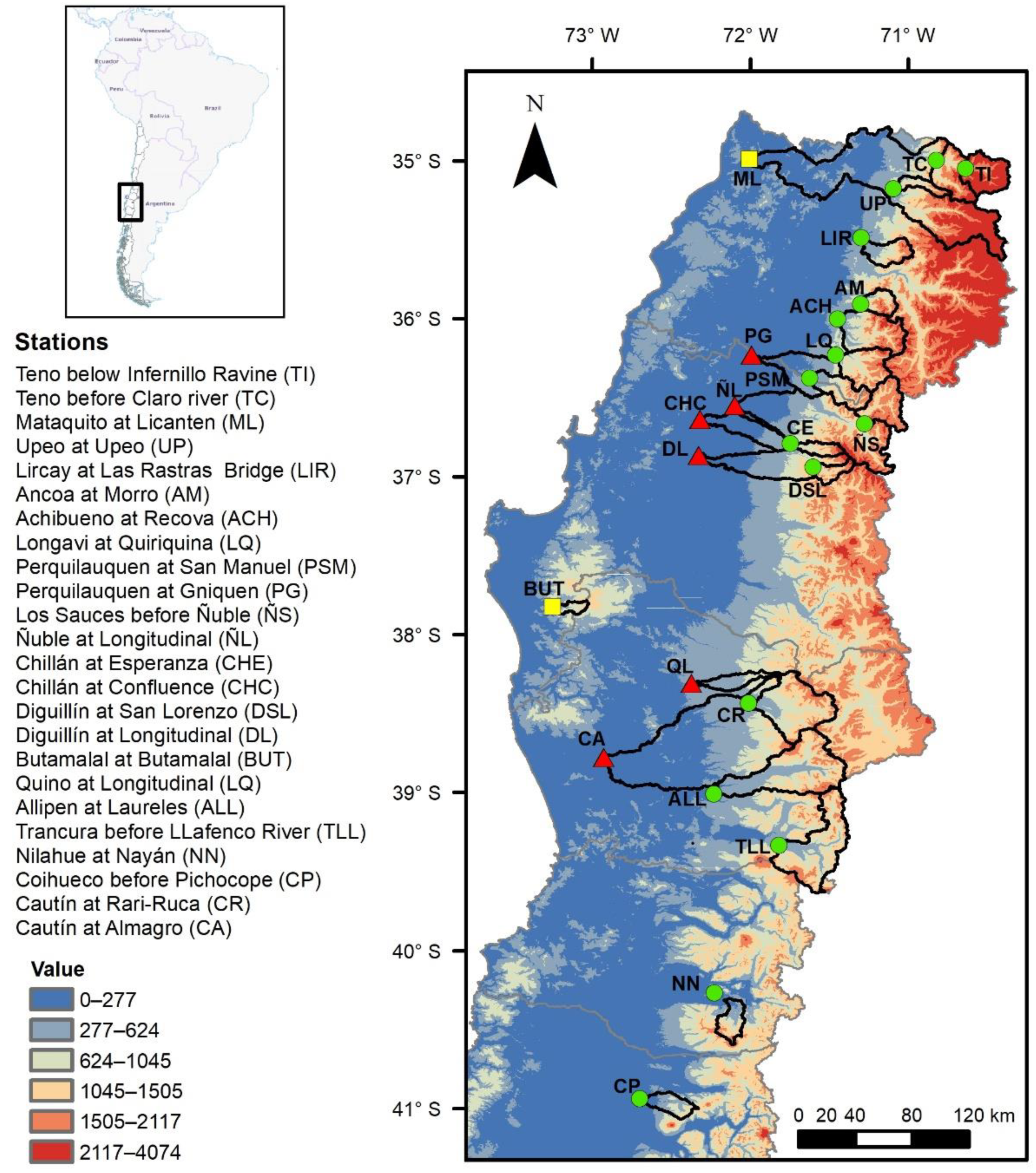
The study area comprises of 24 watersheds located in south-central Chile between latitudes 35° and 41° S (Figure 1), 16 of which are located in the Andes Mountains (AM), 6 in the Central Valley (CV), and 2 in the Coastal Range (CR). The watershed areas range between 123 and 5688 (see Table 1). Watersheds without anthropogenic alterations or with minimal alterations were selected in order to discard anthropogenic effects on the analysis.
In general, the selected watersheds in the central zone present a Mediterranean climate (latitudes ~35–36° S), while those farther south (latitudes ~37–41° S) present a wet climate [15]. In addition, they present a hydrological regime dominated by precipitation in winter and high precipitation variability, with annual averages from 700 to 4000 mm [13,15,16]. Table 1 provides a summary of the geological formations present in each watershed. In accord with the classification carried out by SERNAGEOMIN [14], the geological formations are classified as sedimentary sequences (SS), volcano-sedimentary sequences (SVS), volcanic sequences (VS) and, to a lesser extent, formations associated with intrusive (IF) and metamorphic rocks (MF). These formations consist mainly of alluvial, colluvial, and mass removal deposits, moraine, fluvioglacial, and glaciolacustrine deposits (SS), basaltic to dacitic lavas, epiclastic and pyroclastic rocks (SVS), pyroclastic deposits, mainly rhyolitic, associated with caldera collapse, basaltic to rhyolitic lavas (SV), granodiorites, diorites, tonalites and hornblende (IF), and metaturbidites with low-grade metamorphism, metapelites. and metabasites (MF).
Of the 24 studied watersheds, 16 are on the western slope of the Andes at elevations above 200 m.a.s.l (yellow circles in Figure 1). Most of these watersheds are dominated by formations associated with volcanic and volcano-sedimentary sequences; however, a few (6 watersheds) present a significant portion of intrusive and metamorphic formations [11,12,13,14]. In addition, due to the tectonic uplift of the Andes, most of the watersheds present a rugged topography, with steep slopes of approximately 20° (Table 1). The watersheds located in the Central Valley (6 watersheds, red triangles in Figure 1) are located between 80 and 120 m.a.s.l. and present a geological configuration dominated by sedimentary formations. Despite the dominance of formations of a volcanic origin in their upper parts, the middle and lower zones are characterized by sedimentary deposits (e.g., alluvial, colluvial, and fluvioglacial deposits) originating in the Andes Mountains [14]. Meanwhile, one coastal range watershed (ML) is dominated by sedimentary and volcano-sedimentary formations and the other coastal range watershed (BUT) is dominated by granitic (intrusive) and metamorphic formations resulting from physical and chemical processes.
The geological formations have different characteristics (fractures, porosity, permeability, etc.) that determine the capacity of a watershed to conduct and transmit water, allowing water infiltration, storage, and discharge [17]. Therefore, the predominant geology of a basin can play an important role in the groundwater storage-release process.
For the recession flow analysis average daily flows obtained from the local water authority, the Dirección General de Aguas (DGA), were used. As the data availability periods and gaps vary among all the stream gauge stations, the recording periods depended on the data availability and quality. Periods were selected based on the presence of complete, continuous records; the period with the most complete records was then selected. Data availability in each watershed, among other characteristics, is described in Table 1.
2.2. Recession Flow Analysis
Daily flow data were used for the analysis, discarding the months with the greatest precipitation influence (May–October) in each year of records to represent only periods with low or recession flows [7]. Given the hydro-climatological characteristics of the studied watersheds (Mediterranean climate), precipitation events can be found in the selected periods, which can influence the results. To overcome this fact, precipitation records from rain gauge stations present in each studied watershed were compared with the recession data in the same period in order to eliminate flows associated with precipitation events greater than 0 mm.
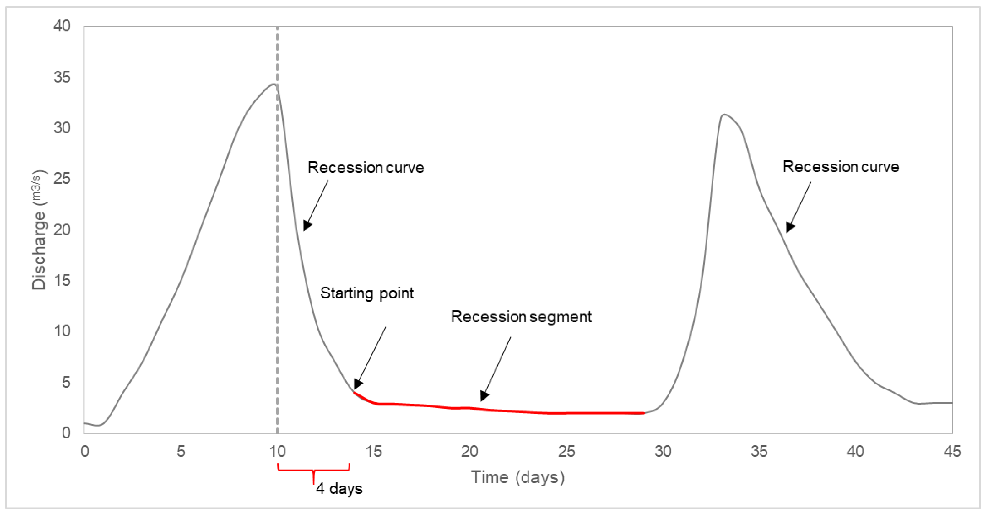
The recession events were identified when was less than zero for at least 6 consecutive days before becoming greater than zero, with the last two days of each selected period discarded to minimize the effect of precipitation processes—surface runoff on the observed flows [5,7]. Therefore, in accord with this criterion, recession periods of 4 or more consecutive days were used (Figure 2).
The theoretical relationship of the temporal variation in the surface discharge, fed by the aquifer, is given by Equation (1) [5]. This relationship indicates that the temporal variation in the recession flows depends on average aquifer discharge. Exponent of the equation represents the linearity of the groundwater storage-release process. If the exponent is not equal to 1, the equation represents an aquifer with a non-linear storage-release relationship, while if b is equal to 1, the aquifer is deemed to be represented by a linear relationship [18].
The employed methodology consisted of plotting the logarithm of the flow change rate (Equation (2)) against the logarithm of average discharge (Equation (3)) during the same period [6,19], where is the time between two consecutive recession days [7]. The logarithmic transformation simplifies the analysis, since Equation (1) becomes linear, as seen in Equation (4). Where is the intercept associated with the hydraulic and geomorphological characteristics of a watershed and is the slope of a line of best fit using least squares, called the “recession slope” [9,20].
In accord with Brutsaert and Nieber [5], recession data can be analyzed using 3 envelopes under the point cloud (3 slopes) obtained from the solution of the Boussinesq equation. The Boussinesq equation describes water drainage from an ideal rectangular aquifer—non-confined and with a width B that drains into a stream. The main assumption is that the aquifer is initially saturated [19,21].
When solving the Boussinesq equation, a slope equal to 1 represents an aquifer with linear drainage over time. A slope of ~3/2 represents a system in which the aquifer water table remains curved over its entire length and throughout the entire drainage process; therefore, the recession drawdown extends over the entire width of the aquifer (slow drainage process). Finally, a slope equal to 3 is obtained when the aquifer that drains the stream is initially saturated; therefore, the drainage is not yet influenced by the no-flow condition at the boundary (quick drainage process) [7,18,19,22]. Oyarzún et al. [19] stated that the surface flow of a river consists of two components: (i) an initial surface runoff component that operates over a relatively short time between a rainfall event and the arrival of the water at the river, i.e., quick drainage, and (ii) a component that infiltrates into the aquifer and is discharged more slowly, i.e., slow flow or baseflow. In other words, if the recession data present a behavior with a slope between 1 and 3/2, the aquifer has been draining for a long time; by contrast, a slope greater than 3/2 (or between 3/2 and 3) represents an aquifer that has been draining for a short time [7].
Brutsaert and Nieber [5] and Shaw and Riha [7] use lower envelope lines with slopes of 3/2 and 3 to identify slow-drainage (long-time) and quick-drainage (short-time) responses of the aquifer, respectively. In order to identify quick or slow drainage behaviors in the recession flow data and associate these behaviors with the predominant geological characteristics of the watershed, lines with slopes of 3/2 and 3 were fitted to the recession data of each watershed using the least-squares method. The slopes were fitted to each watershed assuming that at least 90% of the data points are above the lower envelopes [23].
As the exact position of the lower envelope is uncertain [24], a regression to grouped (bins) data was carried out with the aim of drawing a center line through the recession data. Mendoza et al. [6] mention that the slope of the regressions provides insight into the average basin-wide recession, which helps identify the average behavior of the recession data (dominant drainage regime). To this end, the data were grouped into data bins in accord with the methodology used in Kirchner [9]. To obtain the bins, the recession flows were arranged in descending order, and equal intervals with 5% of the data were obtained [25]. Within each interval an average of log () and log () was calculated, and, using the least-squares method, the value of slope b, which represents the average storage-release behavior of the watershed, was determined.
Finally, to assess the influence of the recession starting point (after the hydrograph peak) on fast or slow groundwater storage behavior according to geological characteristics, slope b was calculated again, varying the starting point. Starting points of 4, 6, 8, 10, 12, and 14 days after the hydrograph peak were considered.
3. Results and Discussion
3.1. Recession Flow Behavior
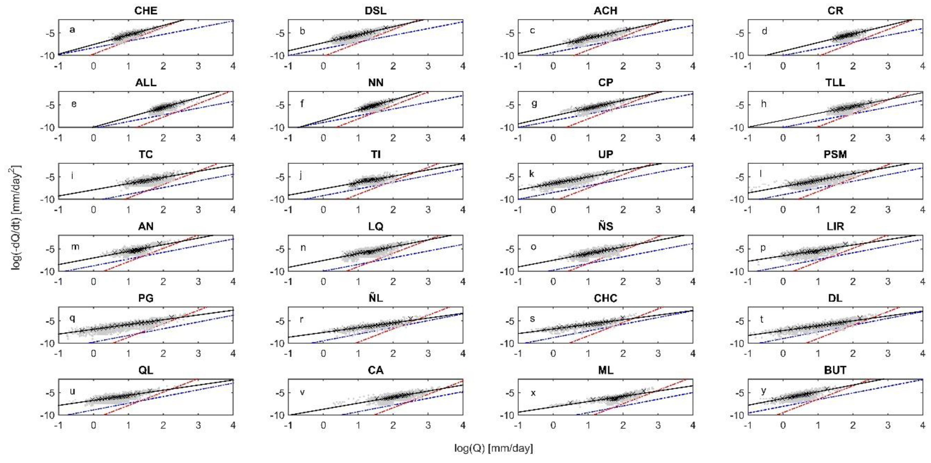
Figure 3 shows the recession graphs of the studied watersheds, as well as the lower envelope of slopes 3/2 and 3 as a reference. In general, three behaviors are observed: watersheds with slopes greater than 3/2, watersheds with slopes near 3/2 and watersheds with slopes less than 3/2. It is observed that the recession flows of mountain watersheds (AM) have a more pronounced slope than those of the watersheds of the Central Valley, which is associated with a geology composed of fractured rocks and lower residence time. These results are consistent with the geology associated with the various watersheds and the geological map published by SERNAGEOMIN [14]. A comparison of the mountain watersheds (Figure 3a–p), which present more pronounced slopes ( > 3/2), with those of the Central Valley (Figure 3q–v), which present a best-fit slope of less than 3/2, indicates that the watersheds located in Central Valley present slow drainage influenced by the sedimentary formations present in the watersheds (see geological formations in Table 1). These geological characteristics influence the storage residence time and the recession flow behavior recorded in this analysis.
Meanwhile, the recession flow behavior of the BUT watershed (Figure 3y), located in the upper zone of the Coastal Range, does not present a clear behavior (Figure 3); therefore, it is not possible to identify what type of behavior predominates there (quick or slow drainage). This behavior may be associated with the geological formations present in the watershed, with a significant proportion of intrusive formations (Table 1). In the case of the ML watershed (Figure 3x), the recession data present a behavior with a slope of less than 3/2. The watershed is located in the low-lying zone of coastal Chile, meaning that it presents a large proportion of sedimentary formations (~40%) and therefore it is similar to watersheds located in the Central Valley. Consequently, ML exhibits slow drainage behavior due to the sedimentary influence that increases groundwater residence time.
In accord with the recession flow behaviors observed in Figure 3, the watersheds located in the Andes Mountains present quick drainage behavior (recession data slope greater than 3/2). According to the geology described by SERNAGEOMIN [14], the watersheds located in the Andes zone exhibit a volcanic influence and typically present a large proportion of fractures. Millares et al. [26] indicate that these systems, in which it is difficult to explain the evolution of baseflow, are associated with a quick groundwater storage response. The fractures form preferential flow paths, which favor groundwater recharge, movement, and release, translating into quick drainage. In addition, in south-central Chile, the Andes Mountains receive much more precipitation than lower-lying areas (e.g., the Central Valley) due to the orographic effect [27] (see mean annual precipitation in Table 1). Thus, it can be inferred that the quick drainage behavior that predominates in these watersheds (located in the AM) is associated with local groundwater recharge and release. In contrast, the Central Valley watersheds present long-term drainage (recession data slope ~1). This is explained by the sedimentary nature of these watersheds [14], the influence of which results in greater groundwater residence time. Stoelzle et al. [4] state that valley aquifers are normally located in unconsolidated sediments with large groundwater deposits that drain slowly but continuously. Therefore, it can be inferred that the slow drainage behavior that predominates in the watersheds of the Central Valley is associated with prolonged groundwater recharge-storage-release processes.
3.2. Predominant Drainage Process
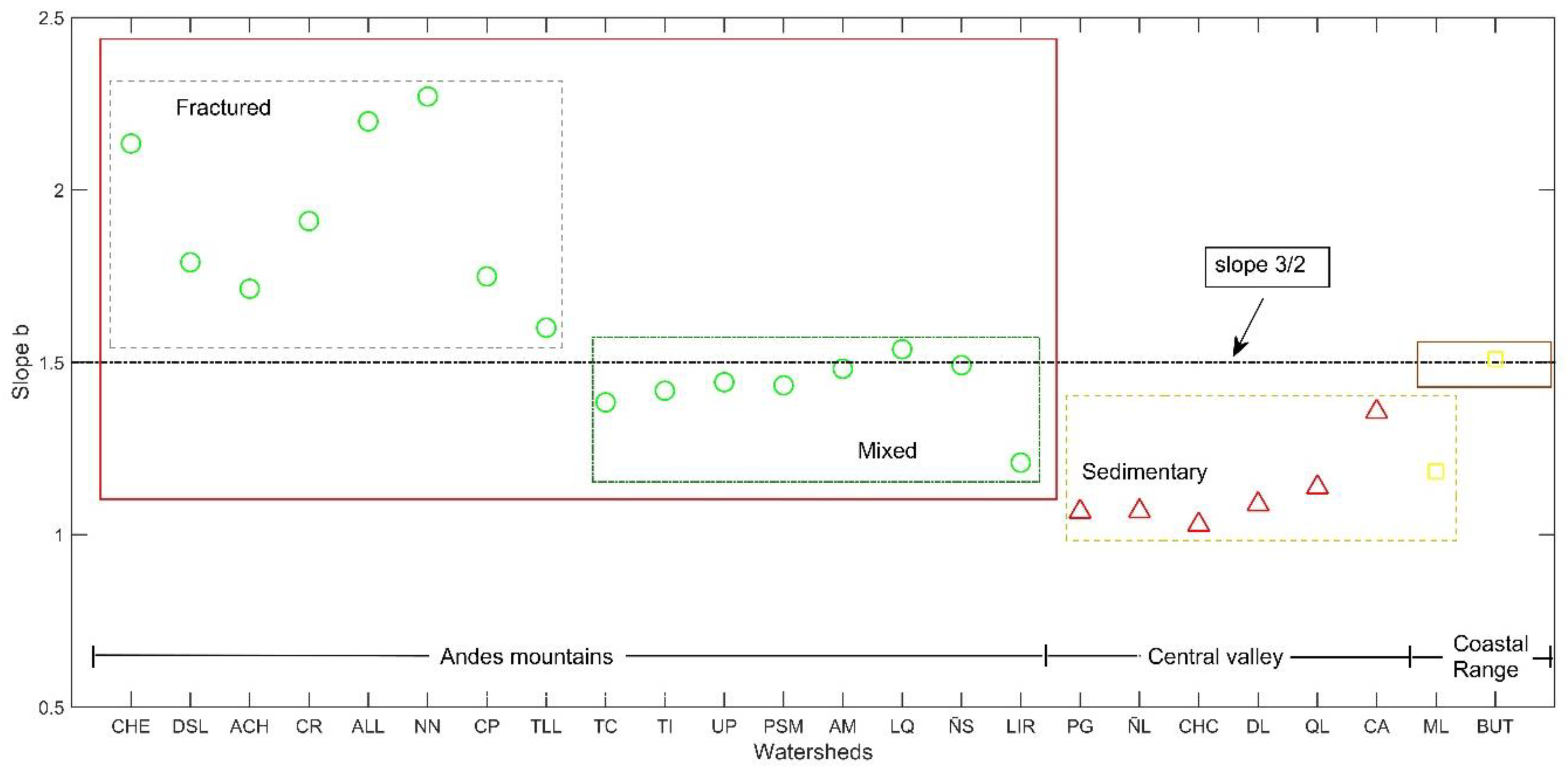
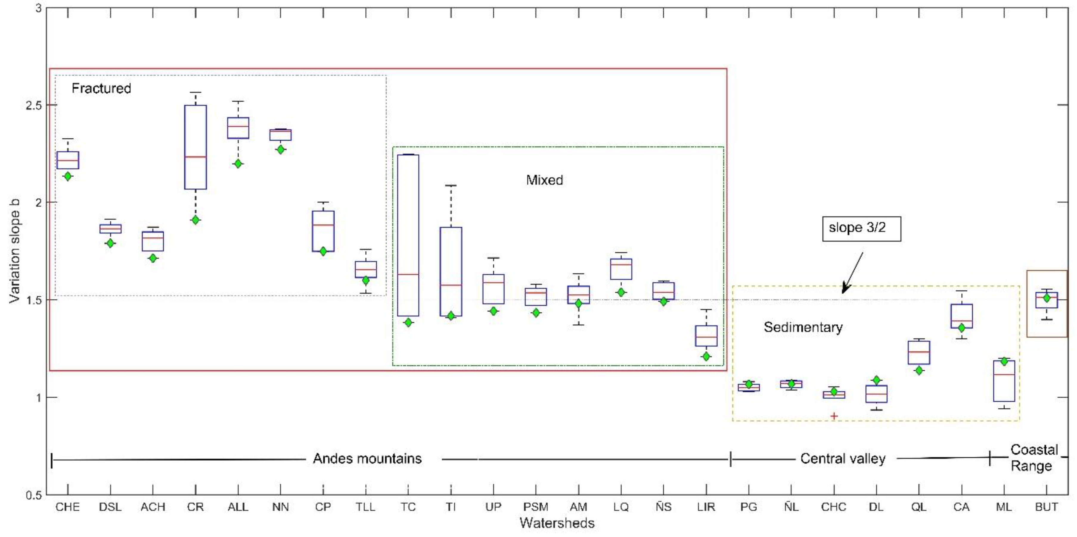
The value of slope obtained by the least-squares (associated with the data bins) is presented in Figure 4. The figure shows a classification by location (Andes Mountains, Central Valley, and Coastal Range) and the proportion of geological formations in each watershed according to Table 1 (fractured influence, mixed influence, sedimentary influence). These results confirm that the recession data (streamflows) from the watersheds of the Andes Mountains present a greater slope than those of the Central Valley. Slope of the recession data from the watersheds of the Andes Mountains presents a higher, broader range (between 1.60 and 2.27), while the watersheds of the Central Valley present a variation between 1.03 and 1.21. Thus, it can be inferred that the storage-discharge behavior of mountain watersheds is strongly influenced by geological formations with fractured characteristics [12], generating greater variability in groundwater storage-release behavior.
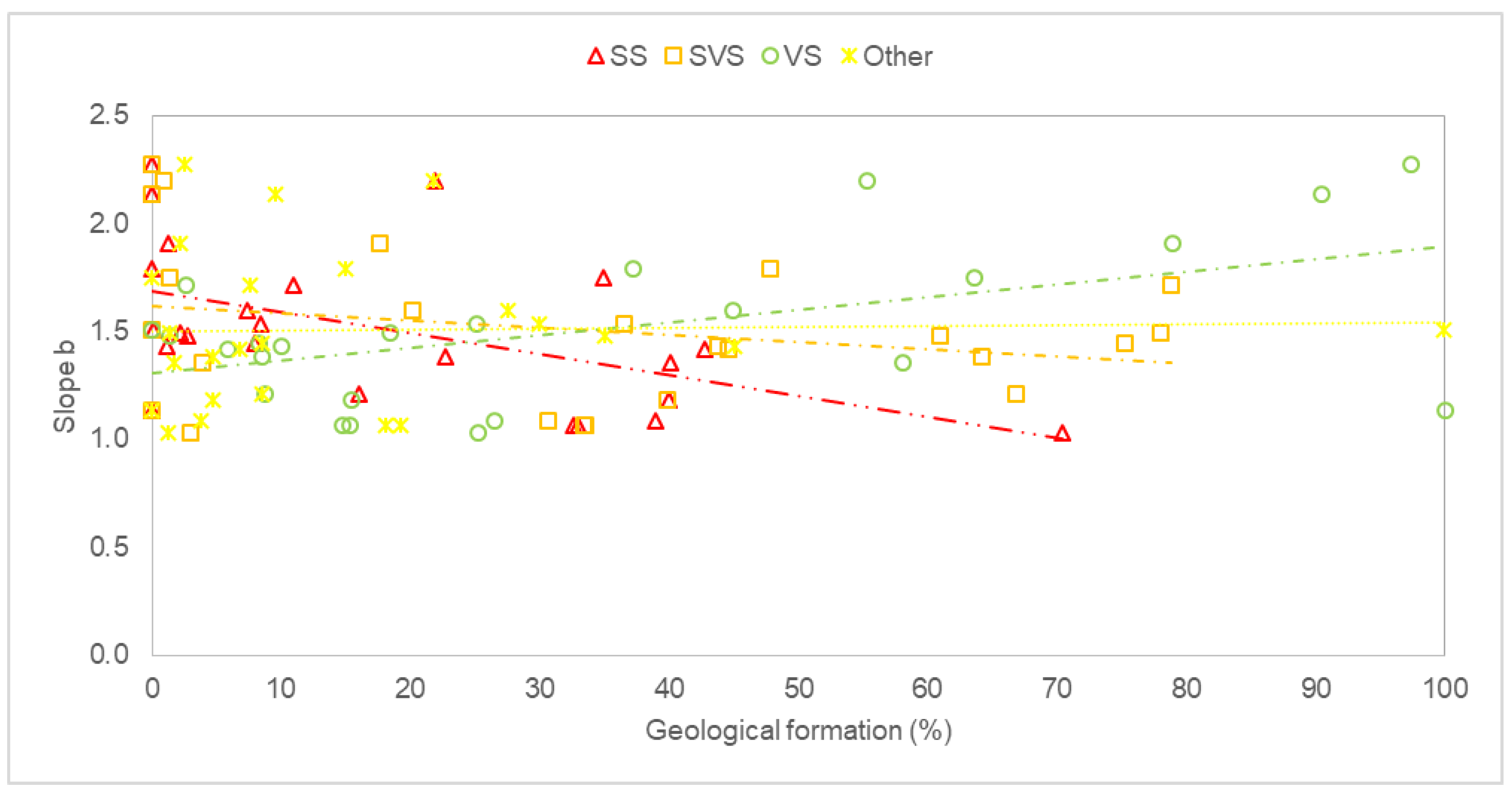
In addition, Figure 4 shows an area with watersheds that present an average slope of around 3/2. Although most of these watersheds are located in the Andes Mountains, this behavior can be attributed to a greater mix of geological formations, composed to a significant extent of a combination of sedimentary, volcano-sedimentary, volcanic, and intrusive sequences (Table 1). As already mentioned, the sedimentary effect influences residence time, which implies a lower slope compared to mountain watersheds with greater fractured volcanic characteristics. The TC, TI, UP, PSM, ÑS watersheds, which present a greater percentage of sedimentary characteristics than the other mountain watersheds (e.g., the CHE, CP, and NN watersheds), are in this group. It is possible that the watersheds, as they present a greater variety of geological formations, along with a lower proportion of formations associated with fractured rock systems, exhibit transient behavior between quick and slow drainage, with slopes close to 3/2. Similar behavior is observed in BUT (slope value of 1.51) due to the proportion of intrusive (68.8%) and metamorphic formations (31.1%) in the watershed, which are associated with granites and metamorphic slates that present a lower degree of fracturing [14]. Figure 5 shows the relationship between the geological formations and the slope . An upward trend of the slope is observed as the percentage of volcanic formations increases; by contrast, a downward trend of the slope is observed as the percentage of sedimentary formations increases. Meanwhile, mixed formations exhibit a neutral trend (slope close to 3/2).
The Diguillín at San Lorenzo (DSL) and Chillán at Esperanza watersheds (CHE) present slope values of 1.79 and 2.13, respectively. This difference is associated with the volcano-sedimentary influence in DSL (47.9%) and the lack of such an influence in CHE (0%), which implies that CHE has a lower aquifer recharge residence time than DSL. These results are consistent with the study of Arumí et al. [28], who state that springs along the river in the DSL watershed allow stable minimum flows, unlike in the Chillán at Esperanza watershed.
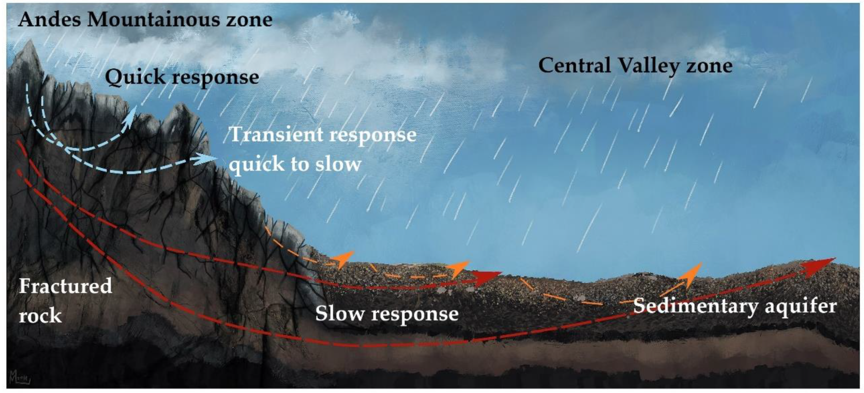
The results indicate different groundwater storage-discharge behaviors among the studied watersheds, suggesting that the watersheds located in the Andes Mountains and Coastal Range have different storage structures; therefore, the aquifers can be represented by different conceptual models. The mountain watersheds (AM), commonly associated with fractured material, present different characteristics than those composed of porous material [26], along with more complex aquifer structures [29]. This greater complexity could be a result of their fractured nature, which favors various flow responses (quick or slow responses). Stoelzle et al. [4] mention that a groundwater storage structure in fractured aquifers could be represented by two parallel deposits, one quick response (associated with precipitation periods) and another slow response. In addition, watersheds associated with sedimentary geology (Central Valley and ML watersheds) with relatively slow aquifer depletion are usually dominated by baseflow [30]. Thus, storage depletion in porous aquifers responds better as a single reservoir system because depletion is relatively slow [4]. Finally, the watersheds with groundwater storage associated with a slope of ~3/2 (which would represent a transition phase between slow and quick storage) could be represented by a non-linear structure because they incorporate a wide range of flows [4,31], although they could also be represented by two linear reservoirs, since different linear reservoir configurations can represent non-linear storage-discharge relationships [32]. Parra et al. [33] obtained similar results evaluating four groundwater storage-release structures (models) in various watersheds with different geological formations (fractured and sedimentary rock). These authors suggest that the two-reservoir structure is suitable for simulating low flows in watersheds with fractured geological characteristics and rugged or steep topography (Andean watersheds) and that a one-reservoir model with a linear response can be adequate for simulating low flows in watersheds with a sedimentary influence or flat topography (Central Valley). Thus, to improve the understanding and representation of different groundwater storage systems, depending on the geology, it can be appropriate to represent these systems in different ways, using either two deposits for mountain watersheds (fractured or mixed influence) or only one deposit for the watersheds of the Central Valley (sedimentary influence). Figure 6 shows a conceptual interpretation of the groundwater storage-release behavior of watersheds in the Andes Mountains and the Central Valley.
3.3. Does the Predominant Drainage Change?
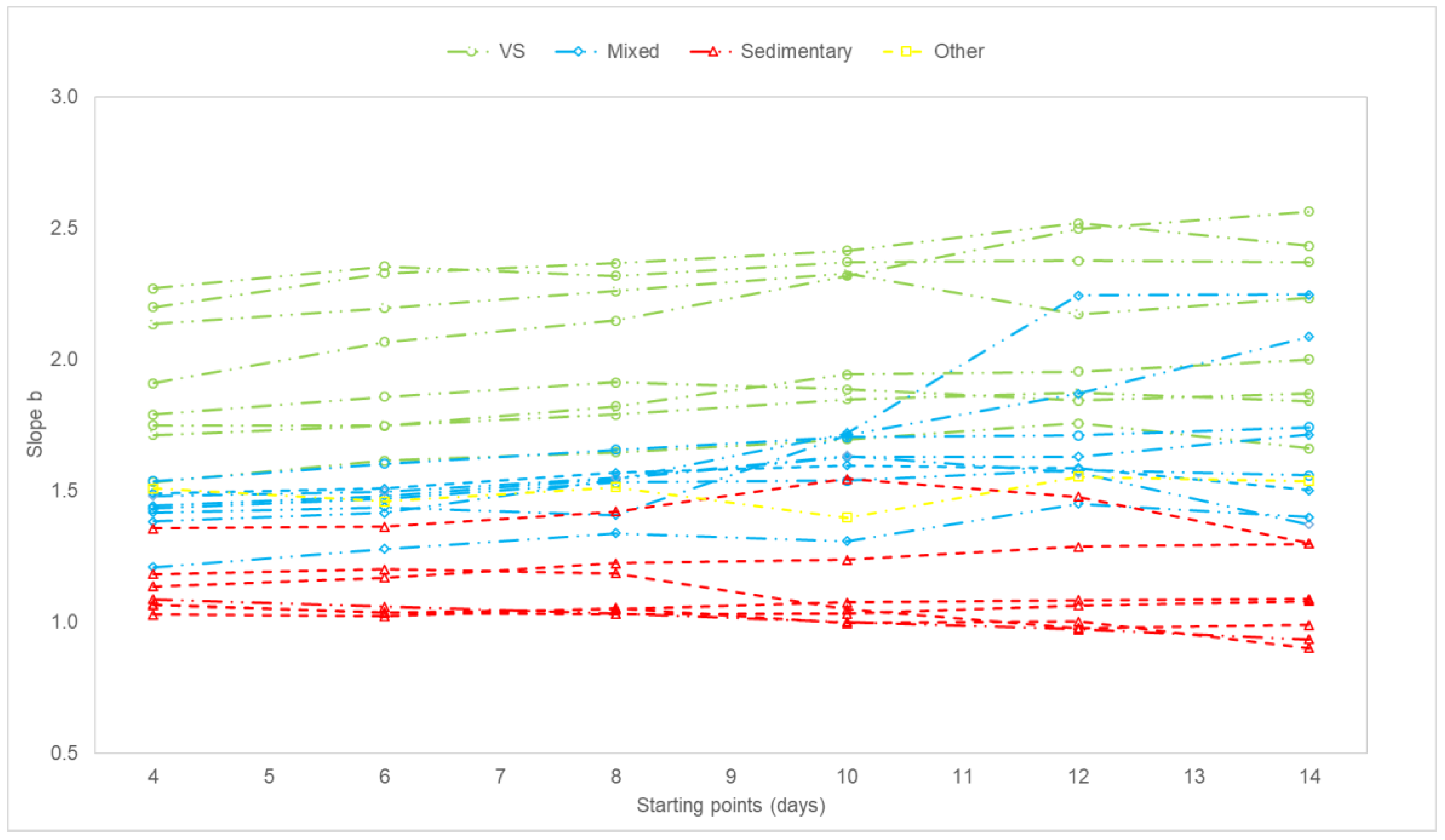
To assess whether the predominant drainage regime (quick or slow groundwater storage behavior) changes with any change in recession data, slope b was calculated for different recession starting points. Figure 7 shows boxplots that contain the six b slopes obtained with the different recession period starting points for all the studied watersheds to see the variation of the slope. It is observed that the average slope is sensitive to the recession starting point. Greater variability in watersheds with volcanic and mixed influence than in watersheds with sedimentary influence is observed. Similar results were found by Chen and Krajewski [34], who analyzed the sensitivity of recession parameters (Equation (1)) at 25 gauges in the Iowa and Cedar River basins in the United States, with drainage areas ranging from 7 to 17,000 km2. The authors assessed the estimation of parameters and under different criteria, finding high parameter sensitivity to the starting point, recession period length and method used. In accord with the obtained results, all of the watersheds showed variation in b when the recession period starting point changed; however, according to the results obtained in this study, in all the starting point scenarios, the mountain watersheds (Andes Mountains) presented quick drainage (b > 3/2), while sedimentary watersheds exhibited slow drainage ( < 3/2), thus reaffirming the link between geology and storage-discharge response (quick or slow response). Meanwhile, in watersheds associated with mixed geology, an upward trend in the average recession slope is observed (as seen in Figure 8). For example, the TC, TI, and UP watersheds present significantly greater variability than the other watersheds (e.g., CHE, DSL, ACH, NN), which could be associated with their mountainous characteristics, with high average slopes (over 20°) and a greater percentage of mixed volcano-sedimentary influence (64.2%, 44.6%, and 75.2%, respectively) compared to those with sedimentary formations (22.7%, 42.7%, and 8%, respectively) and volcanic formations (8.5, 5.8, and 8.3, respectively). The CR watershed, which presents fractured geology, also exhibits greater variability. This might be associated with its average slope of around 14°, which is lower than those of, for example, the DSL and CHE watersheds, which also present volcanic geology (fractured geology). The differences found in the estimated values might be influenced mostly by a combined effect of the geological and topographic characteristics as the average behavior presented a clear difference between the mountain and the Central Valley watersheds in terms of fast and slow drainage results. In general, the obtained behaviors are consistent with the geological characteristics of the watersheds (sedimentary formations associated with slow drainage and volcanic formations with quick drainage), as these characteristics affect their behavior and the response times of the effluent flows of the aquifers [35] (see Figure 8).
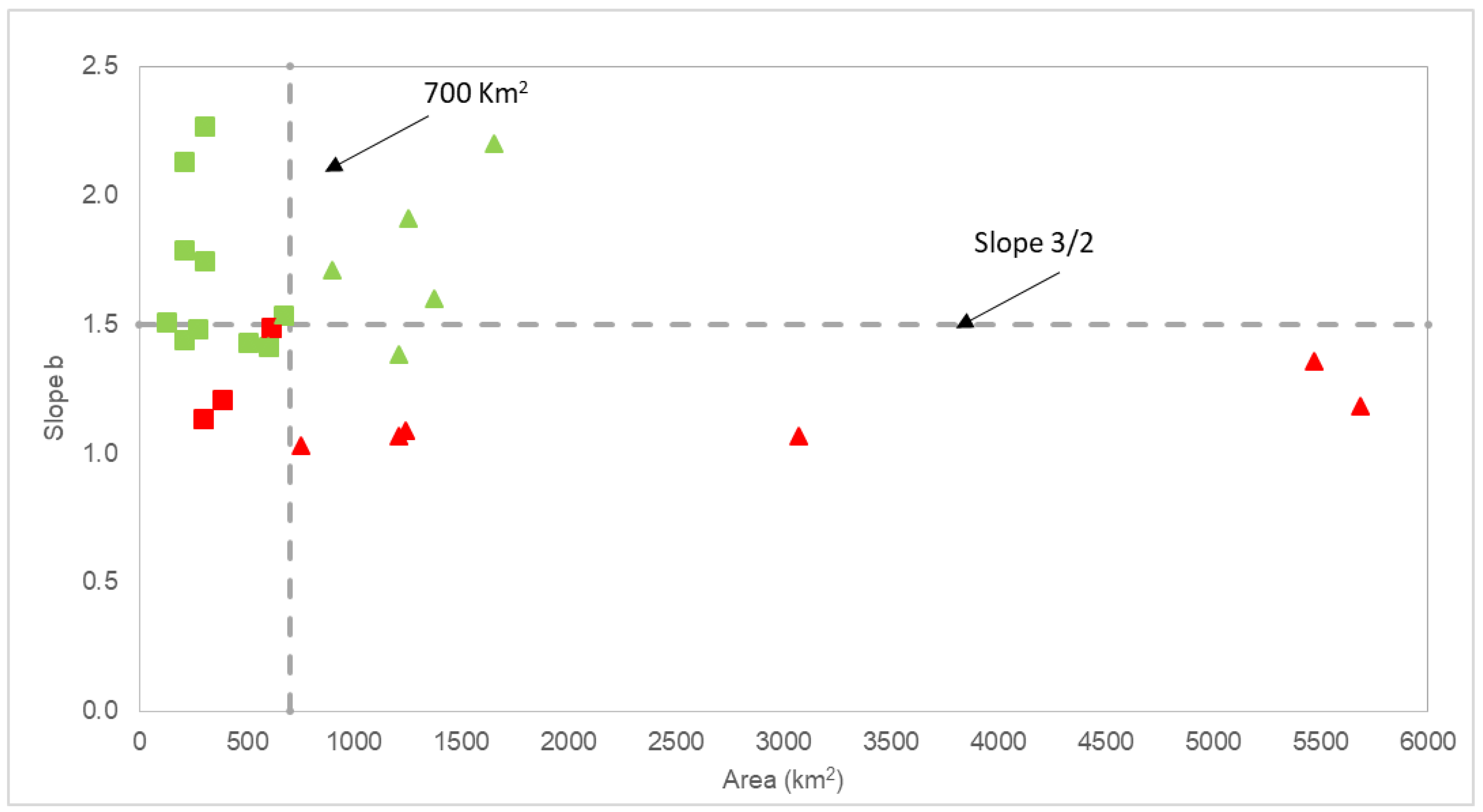
In Figure 9, it is observed that the watersheds with the greatest areas (ML, DL, CHC, PG, and CA) present slower drainage than headwaters or those with smaller areas (e.g., DSL, CHE, PSM, CP, and NN). Similar results were obtained by Hailegeorgis et al. [35], who studied 4 watersheds with areas between ~150 and 3000 km2. The authors stated that the watershed with the greatest area presented the slowest response, while the smallest watersheds presented quick drainage (greater slope in the log (dQ/dt)–log (Q) plot), which is associated with the characteristics of sedimentary or alluvial aquifers.
Understanding the groundwater storage of one or various watersheds is fundamental for meeting human consumption and agricultural needs [36]; therefore, predicting minimum flows becomes a crucial task. In general, conceptual groundwater storage models are used to predict flows; they can be based on a linear [37] or non-linear relationship [38]. However, the selected groundwater model does not necessarily provide an adequate conceptual representation of the characteristics of the watershed and, generally, modelers do not have a priori information on a groundwater storage-release system that can be better represented or simulated by a conceptual model. In accord with the results of this study, the groundwater storage-release systems of the studied watersheds present different behaviors depending on the predominant geological characteristics of each watershed, suggesting the existence of different structures in each set of watersheds. In general, there is no consensus on what structure is appropriate or optimal for predicting minimum flows. For example, Fenicia et al. [39] studied 8 watersheds in Luxembourg with different geological characteristics (marls, sandstones, schist, limestone), concluding that a linear storage model can properly represent the groundwater storage behavior of the watersheds. Chapman [40] indicates that in practical situations a linear storage-discharge model is a good approximation, while Gan and Lou [41] stated that a non-linear model can improve simulation in low-flow periods. Therefore, to properly predict minimum flows, it is necessary to delve into groundwater storage and release processes in order to improve both the quality of the predictions and the representativeness of the simulated processes.
4. Conclusions
This study was focused on using recession analysis to link groundwater storage and release behavior to the predominant geological characteristics of 24 watersheds. It was found that there is a relationship in which watersheds with greater volcanic influence present quick drainage behavior. This implies that water storage-release in this type of watershed is mainly a quick process. In contrast, watersheds with sedimentary characteristics reflect a greater groundwater residence time in the aquifer, which is associated with slow drainage and long-distance recharges. Watersheds with mixed geology present transient behavior between slow and quick drainage. In general, the results suggest that with the recession flow analysis, it is possible to identify different groundwater storage behaviors associated with different geological characteristics, making it a valuable tool for improving the representation and conceptualization of this process in order to advance in the prediction of minimum flows.
Author Contributions
V.P., J.L.A., and E.M. designed the research and analyses; V.P., J.L.A., and E.M. analyzed the data and performed the analyses; V.P., J.L.A., E.M., and J.P. designed the paper, developed the discussion, and wrote the paper.
Funding
This research was funded by CRHIAM, Conicyt/Fondap/15130015 and Dirección de Investigación UCSC DINREG 03/2019.
Acknowledgments
The authors thank the Dirección General de Aguas (National Water Directorate) for providing all the data for the development of this study.
Conflicts of Interest
The authors declare no conflict of interest.
References
- Hood, J.L.; Roy, J.W.; Hayashi, M. Importance of groundwater in the water balance of an alpine headwater lake. Geophys. Res. Lett. 2006, 33, L13405. [Google Scholar] [CrossRef]
- Basile, H.; Seguis, L.; Hiderer, J.; Cohard, J.; Wubda, M.; Descloitres, M.; Benarrosh, N.; Boy, J. Water storage changes as a marker for base flow generation processes in a tropical humid basement catchment (Benin): Insights from hybrid gravimetry. Water Resour. Res. 2015, 51, 8331–8361. [Google Scholar]
- Thomas, B.F.; Vogel, R.M.; Kroll, C.N.; Famiglietti, J.S. Estimation of the baseflow recession constant under human interference. Water Resour. Res. 2013, 49, 7366–7397. [Google Scholar] [CrossRef]
- Stoelzle, M.; Weiler, M.; Stahl, K.; Morhard, A.; Schuetz, T. Is there a superior conceptual groundwater model structure for baseflow simulation? Hydrol. Process. 2015, 29, 1301–1313. [Google Scholar] [CrossRef]
- Brutsaert, W.; Nieber, J.L. Regionalized drought flow hydrographs froma mature glaciated plateau. Water Resour. Res. 1977, 13, 637–643. [Google Scholar] [CrossRef]
- Mendoza, G.F.; Steenhuis, T.S.; Walter, M.T.; Parlange, J.Y. Estimating basin-wide hydraulic parameters of a semi-arid mountainous watershed by recession-flow analysis. J. Hydrol. 2003, 279, 57–69. [Google Scholar] [CrossRef]
- Shaw, S.B.; Riha, S.J. Examining individual recession events instead of a data cloud: Using a modified interpretation of dQ/dt -Q streamflow recession in glaciated watersheds to better inform models of low flow. J. Hydrol. 2012, 434, 46–54. [Google Scholar] [CrossRef]
- Brutsaert, W. Long-term groundwater storage trends estimated from streamflow records: Climatic perspective. Water Resour. Res. 2008, 44. [Google Scholar] [CrossRef]
- Kirchner, J.W. Catchments as simple dynamical systems: Catchment characterization, rainfall-runoff modeling, and doing hydrology backward. Water Resour. Res. 2009, 45, W02429. [Google Scholar] [CrossRef]
- Ajami, H.; Troch, P.; Maddock, T., III; Meixner, T.; Eastoe, C. Quantifying mountain block recharge by means of catchment-scale storage-discharge relationships. Water Resour. Res. 2011, 47. [Google Scholar] [CrossRef] [Green Version]
- Dixon, H.; Murphy, M.; Sparks, S.; Chávez, R.; Naranjo, J.; Dunkley, P.; Young, S.; Gilbert, J.; Pringle, M. The geology of Nevados de Chillán volcano, Chile. Revis. Geol. Chile 1999, 26, 227–253. [Google Scholar] [CrossRef]
- Naranjo, J.; Gilbert, J.; Sparks, R. Geología del Complejo Volcánico Nevados de Chillán, Región del Biobío; Carta Geológica de Chile, Serie Geología Básica: Santiago, Chile, 2008. [Google Scholar]
- Muñoz, E.; Arumí, J.L.; Wagener, T.; Oyarzún, R.; Parra, V. Unraveling complex hydrogeological processes in Andean basins in South-Central Chile: An integrated assessment to understand hydrological dissimilarity. Hydrol. Process. 2016, 30, 4934–4943. [Google Scholar] [CrossRef]
- SERNAGEOMIN. Mapa Geológico de Chile: Versión Digital; Servicio Nacional de Geología y Minería (SERNAGEOMIN): La Serena, Chile, 2003; Volume 4. [Google Scholar]
- Pizarro, R.; Valdes, R.; García-Chevesich, P.; Vallejos, C.; Sangüesa, C.; Morales, C.; Balocchi, F.; Abarza, A.; Fuentes, R. Latitudinal Analysis of Rainfall Intensity and Mean Annual Precipitation in Chile. Chil. J. Agric. Res. 2012, 72, 252–261. [Google Scholar] [CrossRef] [Green Version]
- Bozkurt, D.; Rojas, M.; Boisier, J.P.; Valdivieso, J. Climate change impacts on hydroclimatic regimes and extremes over Andean basins in central Chile. Hydrol. Earth Syst. Sci. Discuss. 2017, 1–29. [Google Scholar] [CrossRef]
- Voeckler, H.; Allen, D.M. Estimating regional-scale fractured bedrock hydraulic conductivity using discrete fracture network (DFN) modeling. Hydrogeol. J. 2012, 20, 1081–1100. [Google Scholar] [CrossRef]
- Sánchez-Murillo, R.; Brooks, E.S.; Elliot, W.J.; Gazel, E.; Boll, J. Baseflow recession analysis in the inland Pacific Northwest of the United States. Hydrogeol. J. 2015, 23, 287–303. [Google Scholar] [CrossRef]
- Oyarzún, R.; Godoy, R.; Núñez, J.; Fairley, J.P.; Oyarzún, J.; Maturana, H.; Freixas, G. Recession flow analysis as a suitable tool for hydrogeological parameter determination in steep, arid basins. J. Arid Environ. 2014, 105, 1–11. [Google Scholar] [CrossRef]
- Vogel, R.; Kroll, C. Regional geohydrologic-geomorphic relationships for the estimation of low-flow statistics. Water Resour. Res. 1992, 28, 2451–2458. [Google Scholar]
- Szilagyi, J.; Parlange, M.B. Baseflow separation based on analytical solutions of the Boussinesq equation. J. Hydrol. 1998, 204, 251–260. [Google Scholar] [CrossRef] [Green Version]
- Brutsaert, W.; Lopez, J.P. Basin-scale geohydrologic drought flow features of riparian aquifers in the southern great plains. Water Resour. Res. 1998, 34, 233–240. [Google Scholar] [CrossRef]
- Malvicini, C.F.; Steenhuis, T.S.; Walter, M.T.; Parlange, J.Y.; Walter, M.F. Evaluation of spring flow in the uplands of Malatom, Leyte, Philippines. Adv. Water Resour. 2005, 28, 1083–1090. [Google Scholar] [CrossRef]
- Troch, P.A.; De Troch, F.P.; Brutsaert, W. Effective water-table depth to describe initial conditions prior to storm rainfall in humidregions. Water Resour. Res. 1993, 29, 427–434. [Google Scholar] [CrossRef]
- Arciniega-Esparza, S.; Breña-Naranjo, J.A.; Pedrozo-Acuña, A.; Appendini, C.M. HYDRORECESSION: A Matlab toolbox for streamflow recession analysis. Comput. Geosci. 2017, 98, 87–92. [Google Scholar] [CrossRef]
- Millares, A.; Polo, M.J.; Losada, M.A. The hydrological response of baseflow in fractured mountain areas. Hydrol. Earth Syst. Sci. 2009, 13, 1261–1271. [Google Scholar] [CrossRef]
- Falvey, M.; Garreaud, R. Wintertime Precipitation Episodes in Central Chile: Associated Meteorological Conditions and Orographic Influences. J. Hydrol. 2007, 8, 171–193. [Google Scholar] [CrossRef]
- Arumí, J.L.; Oyarzún, R.; Muñoz, E.; Rivera, D.; Aguirre, E. Caracterización de Dos Grupos de Manantiales en el Río Diguillín, Chile. Tecnol. Cienc. Agua 2014, 5, 151–158. [Google Scholar]
- Banks, E.W.; Simmons, C.; Love, A.; Cranswick, R.; Werner, A.; Bestland, E.; Wood, M.; Wilson, T. Fractured Bedrock and Saprolite Hydrogeologic Controls on Groundwater/Surface-Water Interaction: A Conceptual Model (Australia). Hydrogeol. J. 2009, 17, 1969–1989. [Google Scholar] [CrossRef]
- Staudinger, M.; Stahl, K.; Seibert, J.; Clark, M.P.; Tallaksen, M. Comparison of hydrological model structures based on recession and low flow simulations. Hydrol. Earth Syst. Sci. 2011, 15, 3447–3459. [Google Scholar] [CrossRef] [Green Version]
- Tallaksen, L. A review of baseflow recession analysis. J. Hydrol. 1995, 65, 349–370. [Google Scholar] [CrossRef]
- Moore, R. Storage-outflow modelling of streamflow recessions, with application to a shallow-soil forested catchment. J. Hydrol. 1997, 198, 260–270. [Google Scholar] [CrossRef]
- Parra, V.; Arumí, J.L.; Muñoz, E. Identifying a Suitable Model for Low-Flow Simulation in Watersheds of South-Central Chile: A Study Based on a Sensitivity Analysis. Water 2019, 11, 1506. [Google Scholar] [CrossRef]
- Chen, B.; Krajewski, W. Analysing individual recession events: Sensitivity of parameter determination to the calculation procedure. Hydrol. Sci. J. 2016, 61, 2887–2901. [Google Scholar] [CrossRef]
- Hailegeorgis, T.T.; Alfredsen, K.; Abdella, Y.S.; Kolberg, S. Evaluation of storage–discharge relationships and recession analysis-based distributed hourly runoff simulation in large-scale, mountainous and snow-influenced catchment. Hydrol. Sci. J. 2016, 61, 2872–2886. [Google Scholar] [CrossRef]
- Murgulet, D.; Murulet, V.; Spalt, N.; Douglas, A.; Hay, R.G. Impact of hydrological alterations on river-groundwater exchange and water quality in a semiarid area: Nueces River, Texas. Sci. Total Environ. 2016, 572, 595–607. [Google Scholar] [CrossRef]
- Uribe, H.; Arumí, J.L.; Gonzáles, L.; Salgado, L. Balances hidrológicos para estimar la recarga de acuíferos en el secano interior, Chile. Tecnol. Cienc. Agua 2003, 8, 17–28. [Google Scholar]
- Bergström, S. The HBV Model: Its Structure and Applications; Swedish Meteorological and Hydrological Institute: Norrköping, Sweden, 1992. [Google Scholar]
- Fenicia, F.; Savenije, H.; Matgen, P.; Pfister, L. Is the groundwater reservoir linear? Learning from data in hydrological modelling. Hydrol. Earth Syst. Sci. 2006, 10, 139–150. [Google Scholar] [CrossRef] [Green Version]
- Chapman, T. A comparison of algorithms for stream flow recession and baseflow separation. Hydrol. Process. 1999, 13, 701–714. [Google Scholar] [CrossRef]
- Gan, R.; Lou, Y. Using the nonlinear aquifer storage–discharge relationship to simulate the base flow of glacier- and snowmelt-dominated basins in Northwest China. Hydrol. Earth Syst. Sci. 2013, 17, 3577–3586. [Google Scholar] [CrossRef]
Figure 1.
Locations of the studied watersheds and gauge stations. Green circles show watersheds located in the Andes Mountains, red triangles show those located in the Central Valley, and yellow squares show those located in the Coastal Range.
Figure 1.
Locations of the studied watersheds and gauge stations. Green circles show watersheds located in the Andes Mountains, red triangles show those located in the Central Valley, and yellow squares show those located in the Coastal Range.

Figure 2.
Schematic of recession segment selection.

Figure 3.
Recession flows for each studied watershed. Gray points indicate the recession flows. The dashed blue line establishes the lower envelope associated with an aquifer with long-term drainage (slope = 3/2) and the dashed red line an aquifer that drains in a short time (slope = 3), respectively. In addition, the linear regression of the data bins is shown. (a–p) are recession graphs of mountain watersheds, while (q–v) are recession graphs of Central Calley watersheds and (x,y) are recession graphs of coastal watersheds. The X marks represent the data bins. The black line is the linear regression applied to the data bins with the least-squares method.

Figure 4.
Slope b obtained by least squares applied to the data bins.

Figure 5.
Relationship between geological formations (%) and the slope . “Other” plots indicate the sum of intrusive and metamorphic formations.
Figure 5.
Relationship between geological formations (%) and the slope . “Other” plots indicate the sum of intrusive and metamorphic formations.

Figure 6.
Conceptual representation of the groundwater storage response in watersheds with fractured and sedimentary influence. The dashed lines represent groundwater recharge in the Andes Mountains and the Central Valley.
Figure 6.
Conceptual representation of the groundwater storage response in watersheds with fractured and sedimentary influence. The dashed lines represent groundwater recharge in the Andes Mountains and the Central Valley.

Figure 7.
The box plot shows the variation in slope b with various recession starting points. In addition, the initially calculated slope is shown as a point of comparison (diamonds).
Figure 7.
The box plot shows the variation in slope b with various recession starting points. In addition, the initially calculated slope is shown as a point of comparison (diamonds).

Figure 8.
Variability in slope b due to the change in the recession starting point. Green circles are watersheds with a predominance of volcanic sequences, blue diamonds are watersheds with mixed geology, red triangles are sedimentary watersheds, and yellow squares indicate a basin with intrusive and metamorphic geological influence.

Figure 9.
The relationship between slope b and watershed areas. Watersheds of the Central Valley (red) and watersheds of the Andes Mountains (green). Rectangles represent watersheds with areas less than 700 km2 and triangles represent watersheds with areas over 700 km2.
Figure 9.
The relationship between slope b and watershed areas. Watersheds of the Central Valley (red) and watersheds of the Andes Mountains (green). Rectangles represent watersheds with areas less than 700 km2 and triangles represent watersheds with areas over 700 km2.


Table 1.
Streamflow monitoring stations, watershed type, and data availability in the studied watersheds. In addition, the geological formation percentages and hydro-meteorological information in each watershed are shown.
Table 1.
Streamflow monitoring stations, watershed type, and data availability in the studied watersheds. In addition, the geological formation percentages and hydro-meteorological information in each watershed are shown.
| Station ID | Area | Data Period | Geological Formation (%) | Relief (°) | Mean Annual Precipitation (mm) | |||||
|---|---|---|---|---|---|---|---|---|---|---|
| Station | ID | (km2) | SS (%) | SVS (%) | VS (%) | IF (%) | MF (%) | AS | ||
| Chillan at Esperanza | CHE | 210 | 1960–2016 | 0.0 | 0.0 | 90.4 | 9.6 | 0.0 | 17.8 | 2200 |
| Diguillín at San Lorenzo | DSL | 207 | 1965–2016 | 0.0 | 47.9 | 37.2 | 14.9 | 0.0 | 23.6 | 2300 |
| Achibueno at the Recova | ACH | 899 | 1986–2016 | 11.0 | 78.8 | 2.6 | 7.6 | 0.0 | 20.1 | 2070 |
| Cautin at Rari-Ruca | CR | 1255 | 1985–2016 | 1.2 | 17.6 | 79.0 | 2.1 | 0.0 | 14.4 | 2330 |
| Río Allipen at Laureles | ALL | 1652 | 1985–2016 | 21.9 | 0.9 | 55.3 | 21.8 | 0.0 | 13 | 2294 |
| Nilahue at Nayan | NN | 304 | 1987–2016 | 0.0 | 0.0 | 97.4 | 2.6 | 0.0 | 11.7 | 2916 |
| Coihueco before Pichicope | CP | 303 | 1987–2016 | 34.9 | 1.4 | 63.7 | 0.0 | 0.0 | 11.0 | 2714 |
| Trancura before Llafenco river | TLL | 1374 | 1970–2016 | 7.4 | 20.2 | 44.9 | 27.5 | 0.0 | 17.0 | 2588 |
| Teno before Claro river | TC | 1206 | 1985–2016 | 22.7 | 64.2 | 8.5 | 4.7 | 0.0 | 22.2 | 1573 |
| Teno Bellow Infernillo Ravine | TI | 601 | 1985–2016 | 42.7 | 44.6 | 5.8 | 6.8 | 0.0 | 22.7 | 1622 |
| Upeo at Upeo | UP | 205 | 1980–2016 | 8.0 | 75.2 | 8.3 | 8.5 | 0.0 | 21.1 | 1354 |
| Perquilauquen at San Manuel | PSM | 504 | 1963–2016 | 1.2 | 43.7 | 10.0 | 45.1 | 0.0 | 18.5 | 2067 |
| Ancoa at Morro | AM | 273 | 1980–2016 | 2.8 | 60.9 | 1.3 | 35.0 | 0.0 | 23.6 | 1998 |
| Longaví at Quiriquina | LQ | 668 | 1966–2016 | 8.4 | 36.6 | 25.1 | 30.0 | 0.0 | 21.2 | 2270 |
| Los Sauces before Ñuble | ÑS | 610 | 1960–2016 | 2.2 | 78.0 | 18.4 | 1.4 | 0.0 | 20.0 | 2398 |
| Lircay at Las Rastras Bridge | LIR | 382 | 1985–2016 | 16.0 | 66.8 | 8.7 | 8.5 | 0.0 | 12.7 | 1621 |
| Perquilauquen at Gniquen | PG | 1205 | 1985–2016 | 32.6 | 33.4 | 14.8 | 19.3 | 0.0 | 11.0 | 1618 |
| Ñuble at Longitudinal | ÑL | 3069 | 1960–2016 | 33.0 | 33.5 | 15.4 | 18.1 | 0.0 | 14.5 | 1900 |
| Chillán to Confluencia | CHC | 754 | 1985–2016 | 70.4 | 3.0 | 25.3 | 1.3 | 0.0 | 10 | 1736 |
| Diguillin at Longitudinal | DL | 1239 | 1985–2016 | 39.0 | 30.7 | 26.5 | 3.8 | 0.0 | 8.1 | 1500 |
| Quino at Longitudinal | QL | 298 | 1969–2016 | 0.0 | 0.0 | 100.0 | 0.0 | 0.0 | 2.4 | 1850 |
| Cautin at Almagro | CA | 5470 | 1985–2016 | 40.1 | 3.9 | 58.1 | 1.0 | 0.7 | 6.0 | 1838 |
| Mataquito at Licanten | ML | 5688 | 1972–2016 | 40.0 | 39.8 | 15.5 | 4.0 | 0.7 | 11.2 | 1242 |
| Butamalal at Butamalal | BUT | 123 | 1985–2016 | 0.1 | 0.0 | 0.0 | 68.8 | 31.1 | 9.3 | 1483 |
SS: sedimentary; SVS: volcano-sedimentary; VS: volcanic; IF: intrusive and MI: metamorphic; AS: average slope; MAP: mean annual precipitation (mm). The hydro-meteorological data were obtained from the historical database of stations controlled by the DGA.
© 2019 by the authors. Licensee MDPI, Basel, Switzerland. This article is an open access article distributed under the terms and conditions of the Creative Commons Attribution (CC BY) license (http://creativecommons.org/licenses/by/4.0/).
Share and Cite
MDPI and ACS Style
Parra, V.; Arumí, J.L.; Muñoz, E.; Paredes, J. Characterization of the Groundwater Storage Systems of South-Central Chile: An Approach Based on Recession Flow Analysis. Water 2019, 11, 2324. https://doi.org/10.3390/w11112324
AMA Style
Parra V, Arumí JL, Muñoz E, Paredes J. Characterization of the Groundwater Storage Systems of South-Central Chile: An Approach Based on Recession Flow Analysis. Water. 2019; 11(11):2324. https://doi.org/10.3390/w11112324
Chicago/Turabian StyleParra, Víctor, José Luis Arumí, Enrique Muñoz, and Jerónimo Paredes. 2019. "Characterization of the Groundwater Storage Systems of South-Central Chile: An Approach Based on Recession Flow Analysis" Water 11, no. 11: 2324. https://doi.org/10.3390/w11112324
Note that from the first issue of 2016, this journal uses article numbers instead of page numbers. See further details here.