Gully Erosion Susceptibility Mapping Using Multivariate Adaptive Regression Splines—Replications and Sample Size Scenarios


Abstract
:1. Introduction
2. Materials and Methods
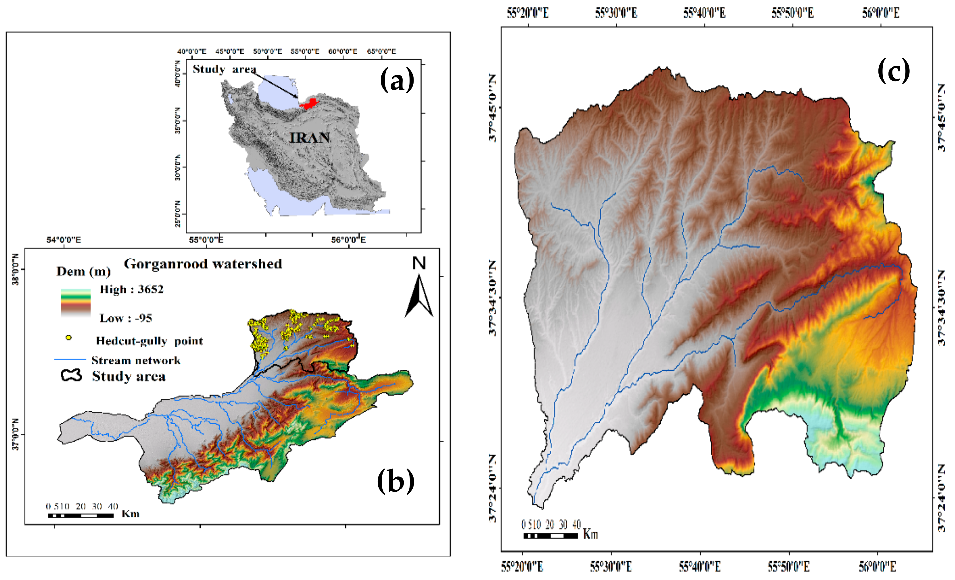
2.1. Study Area
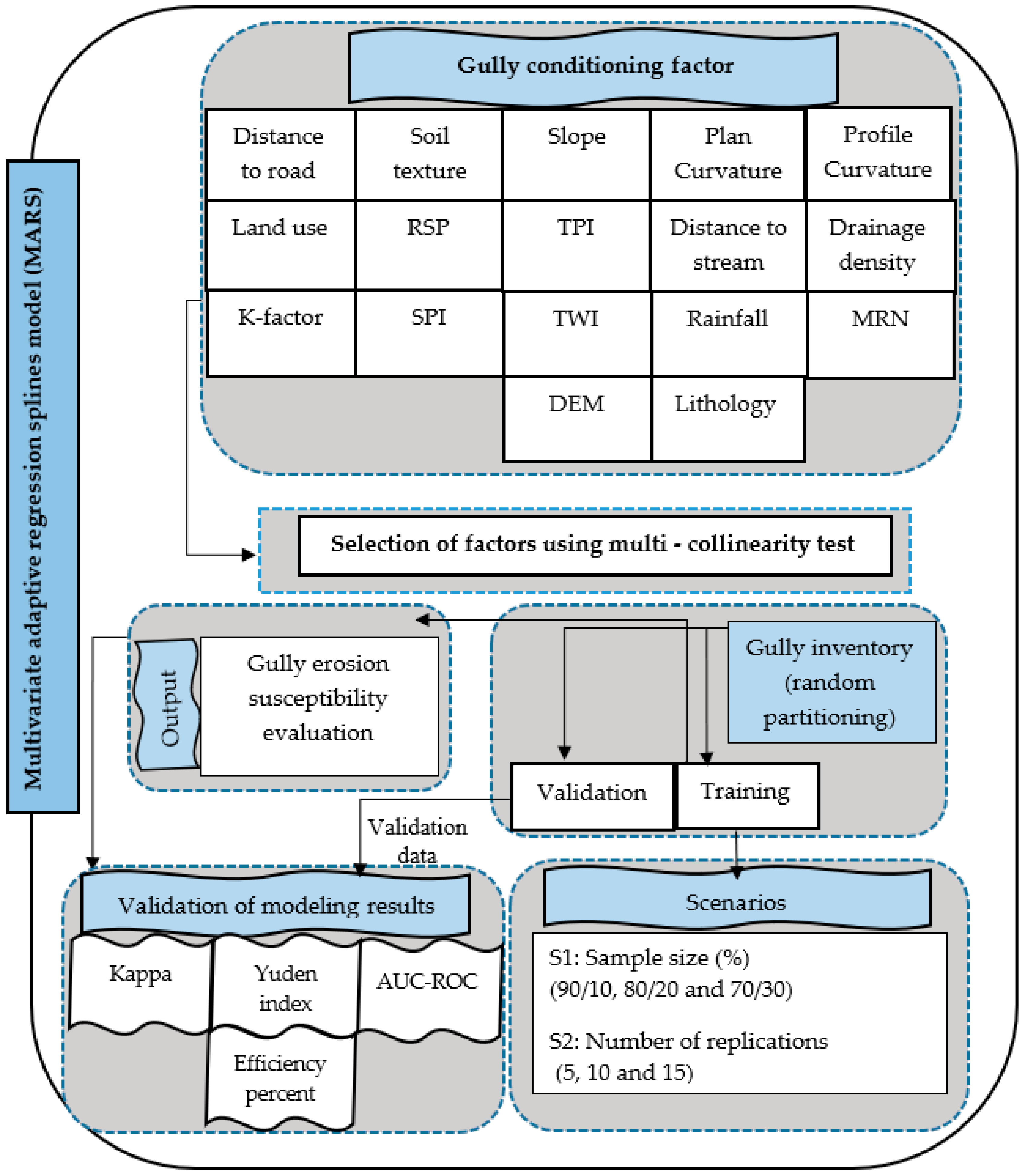
2.2. Methodology
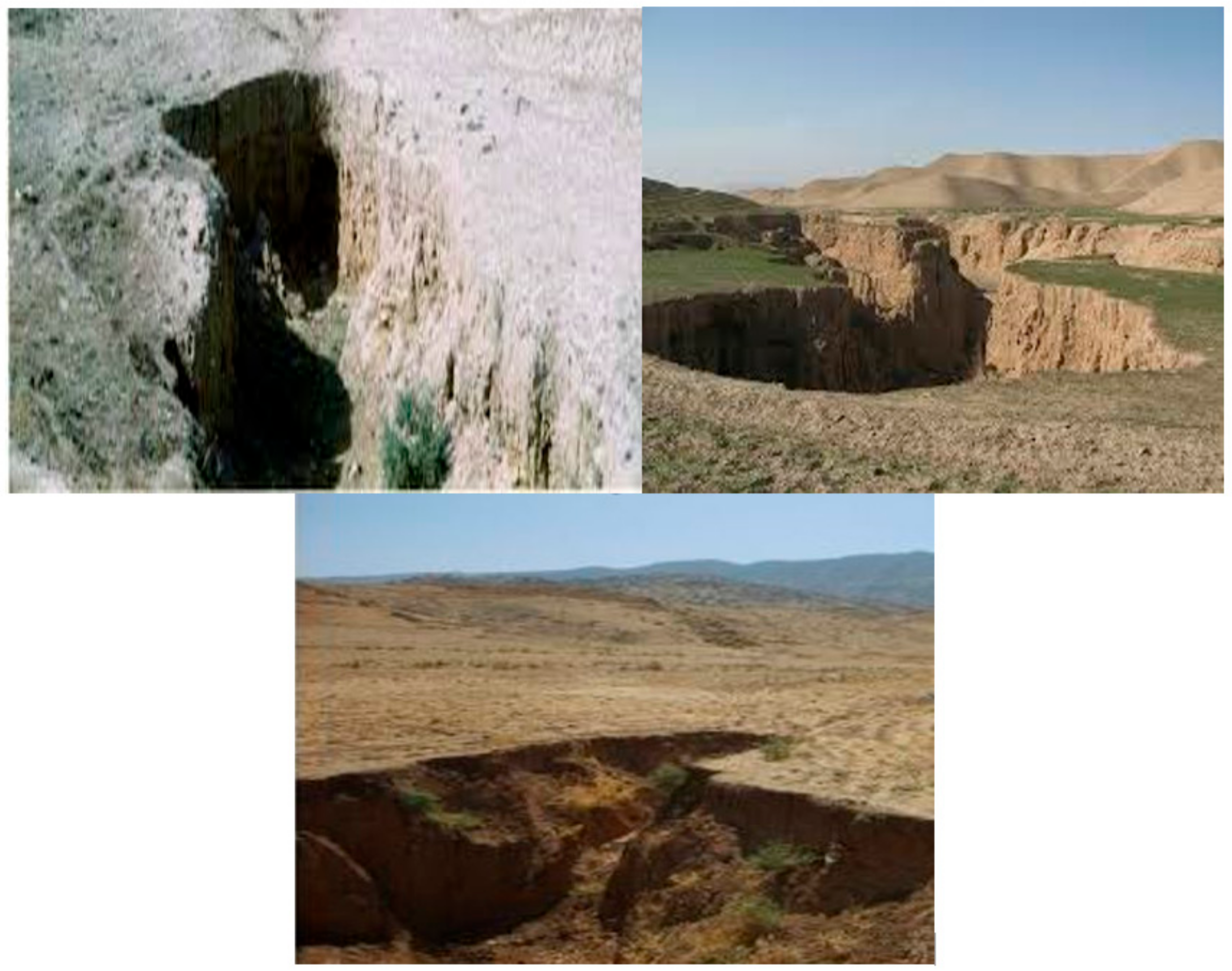
2.2.1. Gully Erosion Inventory Mapping
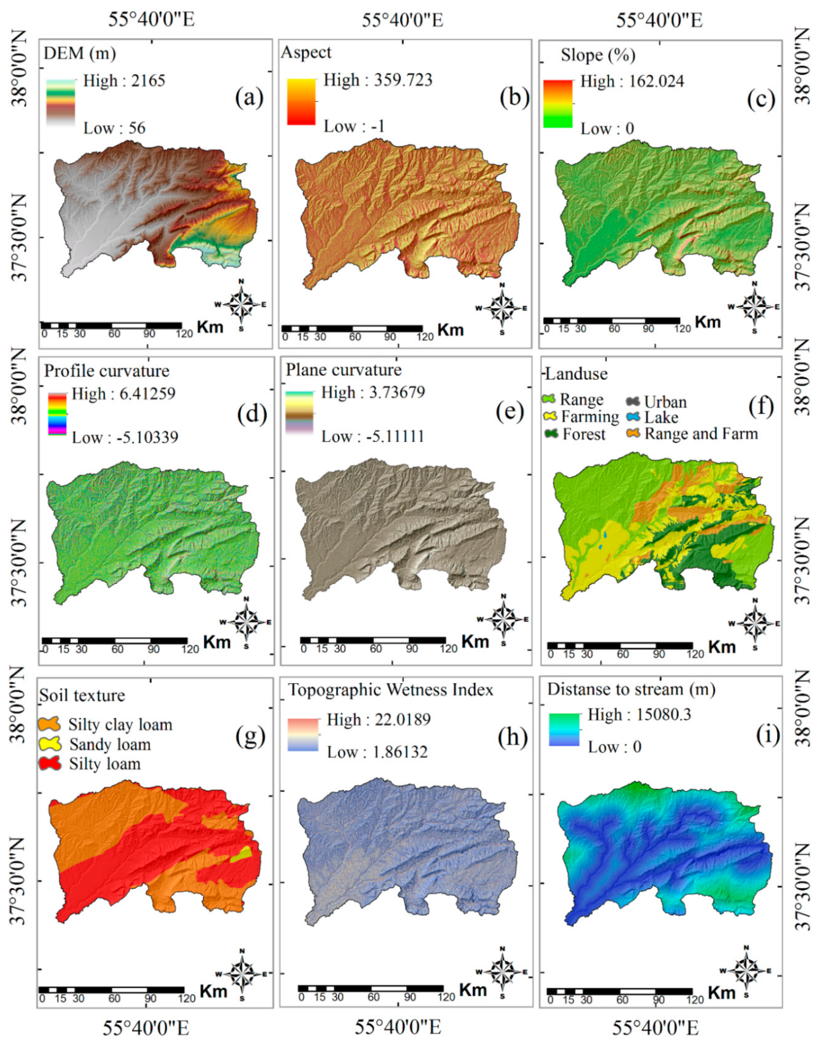
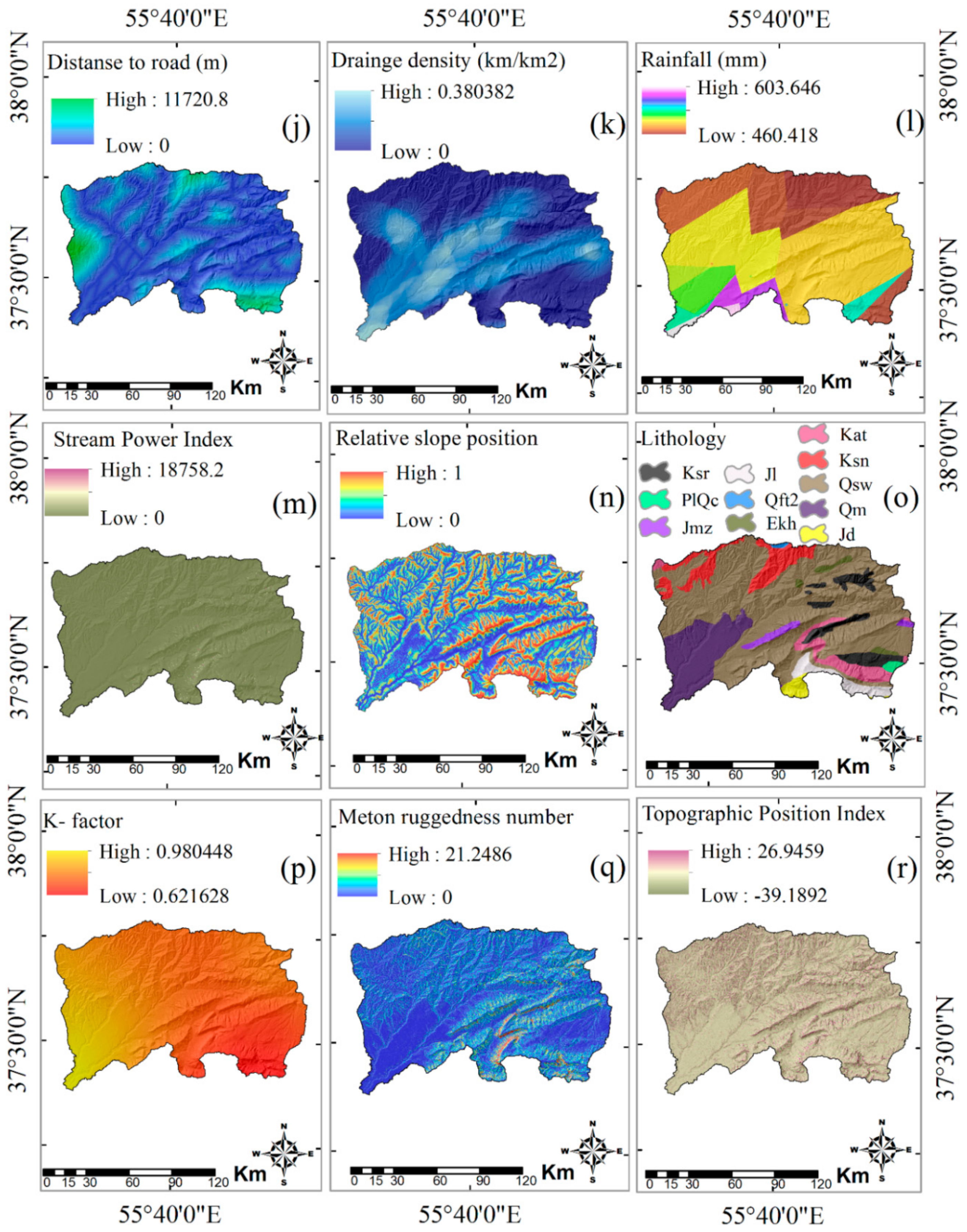
2.2.2. Gully Erosion Predictor Variables (GEPV)
2.3. Multi-Collinearity Test
2.4. Multivariate Adaptive Regression Splines (MARS Model)
Evaluation of the Model
3. Results
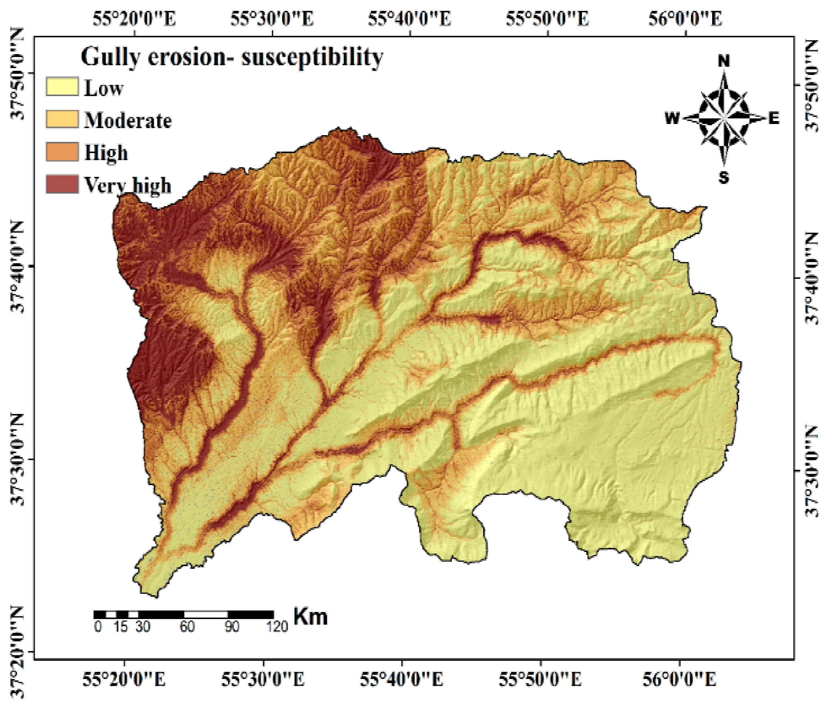
3.1. Gully Erosion Susceptibility Model
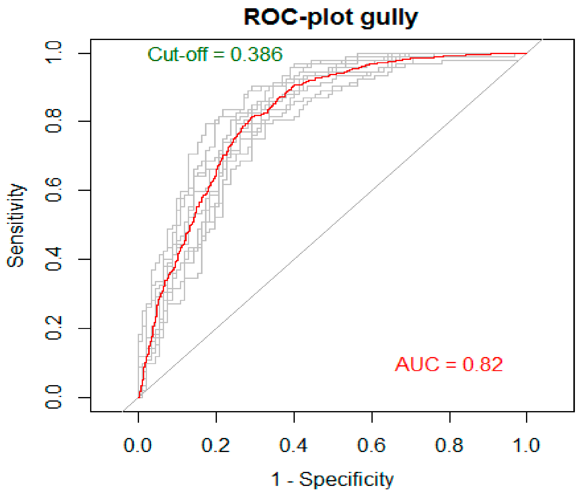
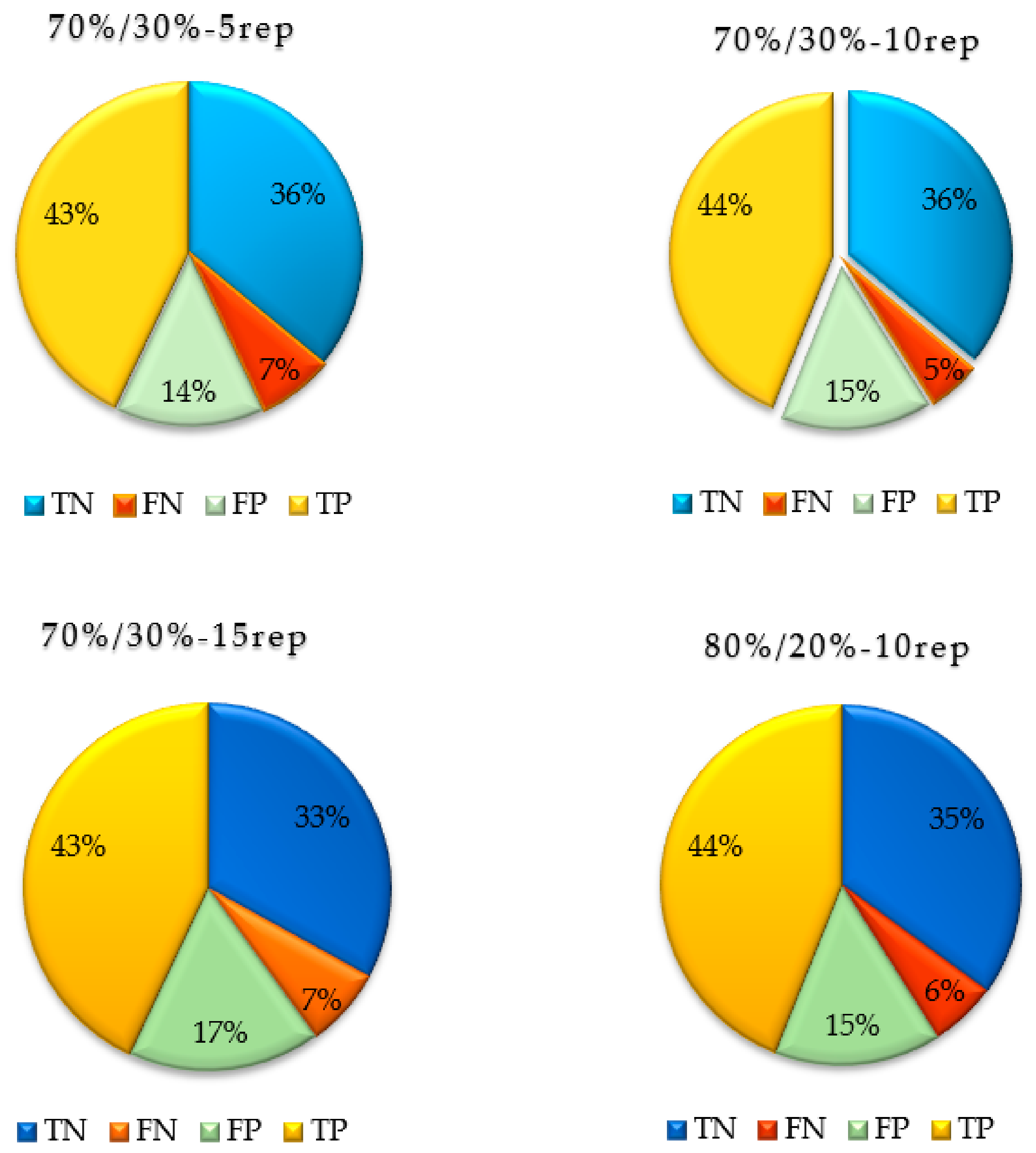
3.2. Evaluation of the Susceptibility in Gully Erosion
4. Discussion
5. Conclusions
Author Contributions
Funding
Acknowledgments
Conflicts of Interest
References
- Lal, R. Offsetting global CO2 emissions by restoration of degraded soils and intensification of world agriculture and forestry. Land Degrad. Dev. 2003, 14, 309–322. [Google Scholar] [CrossRef]
- Kosmas, C.; Danalatos, N.; Cammeraat, L.H.; Chabart, M.; Diamantopoulos, J.; Farand, R.; Gutierrez, L.; Jacob, A.; Marques, H.; Martinez-Fernandez, J.; et al. The effect of land use on runoff and soil erosion rates under Mediterranean conditions. Catena 1997, 29, 45–59. [Google Scholar] [CrossRef]
- Vandekerckhove, L.; Poesen, J.; Oostwoud Wijdenes, D.; Gyssels, G.; Beuselinck, L.; de Luna, E. Characteristics and controlling factors of bank gullies in two semi-arid mediterranean environments. Geomorphology 2000, 33, 37–58. [Google Scholar] [CrossRef]
- Vanwalleghem, T.; Poesen, J.; Nachtergaele, J.; Verstraeten, G. Characteristics, controlling factors and importance of deep gullies under cropland on loess-derived soils. Geomorphology 2005, 69, 76–91. [Google Scholar] [CrossRef]
- Chaplot, V.; Giboire, G.; Marchand, P.; Valentin, C. Dynamic modelling for linear erosion initiation and development under climate and land-use changes in northern Laos. Catena 2005, 63, 318–328. [Google Scholar] [CrossRef]
- Li, Y. Gully erosion: Impacts, factors and control. Catena 2005, 63, 132–153. [Google Scholar]
- Imeson, A.C.; Kwaad, F. Gully types and gully prediction. Geogr. Tydschr. 1980, 14, 430–441. [Google Scholar]
- Angileri, S.E.; Conoscenti, C.; Hochschild, V.; Märker, M.; Rotigliano, E.; Agnesi, V. Water Erosion Susceptibility Mapping by Applying Stochastic Gradient Treeboost to the Imera Meridionale River Basin (Sicily, Italy); Elsevier: Amsterdam, The Netherlands, 2016; Volume 262, ISBN 3909123864643. [Google Scholar]
- Conforti, M.; Aucelli, P.P.C.; Robustelli, G.; Scarciglia, F. Geomorphology and GIS analysis for mapping gully erosion susceptibility in the Turbolo stream catchment (Northern Calabria, Italy). Nat. Hazards 2011, 56, 881–898. [Google Scholar] [CrossRef]
- Govers, G.; Giménez, R.; Van Oost, K. Rill erosion: Exploring the relationship between experiments, modelling and field observations. Earth Sci. Rev. 2007, 84, 87–102. [Google Scholar] [CrossRef]
- Guzzetti, F.; Reichenbach, P.; Ardizzone, F.; Cardinali, M.; Galli, M. Estimating the quality of landslide susceptibility models. Geomorphology 2006, 81, 166–184. [Google Scholar] [CrossRef]
- Carrara, A.; Pike, R.J. GIS technology and models for assessing landslide hazard and risk. Geomorphology 2008, 3, 257–260. [Google Scholar] [CrossRef]
- Vergari, F.; Della Seta, M.; Del Monte, M.; Fredi, P.; Palmieri, E.L. Landslide susceptibility assessment in the Upper Orcia Valley (Southern Tuscany, Italy) through conditional analysis: A contribution to the unbiased selection of causal factors. Nat. Hazards Earth Syst. Sci. 2011, 11, 1475. [Google Scholar] [CrossRef]
- Pozdnoukhov, A.; Matasci, G.; Kanevski, M.; Purves, R.S. Spatio-temporal avalanche forecasting with Support Vector Machines. Nat. Hazards Earth Syst. Sci. 2011, 11, 367–382. [Google Scholar] [CrossRef] [Green Version]
- Costanzo, D.; Cappadonia, C.; Conoscenti, C.; Rotigliano, E. Exporting a Google Earth™ aided earth-flow susceptibility model: A test in central Sicily. Nat. Hazards 2012, 61, 103–114. [Google Scholar] [CrossRef]
- Ballabio, C.; Sterlacchini, S. Support vector machines for landslide susceptibility mapping: The Staffora River Basin case study, Italy. Math. Geosci. 2012, 44, 47–70. [Google Scholar] [CrossRef]
- Conoscenti, C.; Ciaccio, M.; Caraballo-Arias, N.A.; Gómez-Gutiérrez, Á.; Rotigliano, E.; Agnesi, V. Assessment of susceptibility to earth-flow landslide using logistic regression and multivariate adaptive regression splines: A case of the Belice River basin (western Sicily, Italy). Geomorphology 2015, 242, 49–64. [Google Scholar] [CrossRef]
- Magliulo, P. Soil erosion susceptibility maps of the Janare Torrent Basin (Southern Italy). J. Maps 2010, 6, 435–447. [Google Scholar] [CrossRef] [Green Version]
- Magliulo, P. Assessing the susceptibility to water-induced soil erosion using a geomorphological, bivariate statistics-based approach. Environ. Earth Sci. 2012, 67, 1801–1820. [Google Scholar] [CrossRef]
- Conoscenti, C.; Agnesi, V.; Angileri, S.; Cappadonia, C.; Rotigliano, E.; Märker, M. A GIS-based approach for gully erosion susceptibility modelling: A test in Sicily, Italy. Environ. Earth Sci. 2013, 70, 1179–1195. [Google Scholar] [CrossRef]
- Lucà, F.; Conforti, M.; Robustelli, G. Comparison of GIS-based gullying susceptibility mapping using bivariate and multivariate statistics: Northern Calabria, South Italy. Geomorphology 2011, 134, 297–308. [Google Scholar] [CrossRef]
- Conoscenti, C.; Angileri, S.; Cappadonia, C.; Rotigliano, E.; Agnesi, V.; Märker, M. Gully erosion susceptibility assessment by means of GIS-based logistic regression: A case of Sicily (Italy). Geomorphology 2014, 204, 399–411. [Google Scholar] [CrossRef] [Green Version]
- Geissen, V.; Kampichler, C.; López-de Llergo-Juárez, J.J.; Galindo-Acántara, A. Superficial and subterranean soil erosion in Tabasco, tropical Mexico: Development of a decision tree modeling approach. Geoderma 2007, 139, 277–287. [Google Scholar] [CrossRef]
- Märker, M.; Pelacani, S.; Schröder, B. A functional entity approach to predict soil erosion processes in a small Plio-Pleistocene Mediterranean catchment in Northern Chianti, Italy. Geomorphology 2011, 125, 530–540. [Google Scholar] [CrossRef]
- Gutiérrez, Á.G.; Schnabel, S.; Contador, J.F.L. Using and comparing two nonparametric methods (CART and MARS) to model the potential distribution of gullies. Ecol. Model. 2009, 220, 3630–3637. [Google Scholar] [CrossRef]
- Gomez Gutierrez, A.; Schnabel, S.; Felicísimo, Á.M. Modelling the occurrence of gullies in rangelands of southwest Spain. Earth Surf. Process. Landf. J. Br. Geomorphol. Res. Gr. 2009, 34, 1894–1902. [Google Scholar] [CrossRef]
- Gómez-Gutiérrez, Á.; Conoscenti, C.; Angileri, S.E.; Rotigliano, E.; Schnabel, S. Using topographical attributes to evaluate gully erosion proneness (susceptibility) in two mediterranean basins: Advantages and limitations. Nat. Hazards 2015, 79, 291–314. [Google Scholar] [CrossRef]
- Zabihi, M.; Pourghasemi, H.R.; Motevalli, A.; Zakeri, M.A. Gully erosion modeling using GIS-based data mining techniques in Northern Iran: A comparison Between Boosted Regression Tree and Multivariate Adaptive Regression Spline. In Natural Hazards GIS-Based Spatial Modeling Using Data Mining Techniques; Springer: Cham, Switzerland, 2019; pp. 1–26. [Google Scholar]
- Rahmati, O.; Tahmasebipour, N.; Haghizadeh, A.; Pourghasemi, H.R.; Feizizadeh, B. Evaluation of different machine learning models for predicting and mapping the susceptibility of gully erosion. Geomorphology 2017, 298, 118–137. [Google Scholar] [CrossRef]
- Nazari Samani, A.; Ahmadi, H.; Mohammadi, A.; Ghoddousi, J.; Salajegheh, A.; Boggs, G.; Pishyar, R. Factors controlling gully advancement and models evaluation (Hableh Rood Basin, Iran). Water Resour. Manag. 2010, 24, 1531–1549. [Google Scholar] [CrossRef]
- Friedman, J.H. Multivariate adaptive regression splines. Ann. Stat. 1991, 19, 1–67. [Google Scholar] [CrossRef]
- Water Resources Company of Golestan (WRCG). Precipitation and Temperature Reports. Available online: http://www.gsrw.ir/Default.aspx (accessed on 15 May 2013).
- Lee, S.; Ryu, J.-H.; Kim, I.-S. Landslide susceptibility analysis and its verification using likelihood ratio, logistic regression, and artificial neural network models: Case study of Youngin, Korea. Landslides 2007, 4, 327–338. [Google Scholar] [CrossRef]
- Pradhan, B. Flood Susceptible Mapping and Risk Area Delineation Using Logistic Regression, GIS and Remote Sensing. J. Spat. Hydrol. 2009, 9, 1–18. [Google Scholar]
- Cama, M.; Lombardo, L.; Conoscenti, C.; Rotigliano, E. Improving transferability strategies for debris flow susceptibility assessment: Application to the Saponara and Itala catchments (Messina, Italy). Geomorphology 2017, 288, 52–65. [Google Scholar] [CrossRef]
- Rotigliano, E.; Martinello, C.; Agnesi, V.; Conoscenti, C. Evaluation of debris flow susceptibility in El Salvador (CA): A comparison between Multivariate Adaptive Regression Splines (MARS) and Binary Logistic Regression (BLR). Hung. Geogr. Bull. 2018, 67, 361–373. [Google Scholar] [CrossRef]
- Conoscenti, C.; Rotigliano, E.; Cama, M.; Caraballo-Arias, N.A.; Lombardo, L.; Agnesi, V. Exploring the Effect of Absence Selection on Landslide Susceptibility Models: A Case Study in Sicily, Italy; Elsevier: Amsterdam, The Netherlands, 2016; Volume 261, ISBN 3909123864. [Google Scholar]
- Kia, M.B.; Pirasteh, S.; Pradhan, B.; Mahmud, A.R.; Sulaiman, W.N.A.; Moradi, A. An artificial neural network model for flood simulation using GIS: Johor River Basin, Malaysia. Environ. Earth Sci. 2012, 67, 251–264. [Google Scholar] [CrossRef]
- Lee, M.J.; Kang, J.; Jeon, S. Application of Frequency Ratio Model and Validation for Predictive Flooded Area Susceptibility Mapping Using GIS. In Proceedings of the 2012 IEEE international Geoscience and Remote Sensing Symposium; IEEE: Piscataway, NJ, USA, 2012; pp. 895–898. [Google Scholar]
- Youssef, A.M.; Pourghasemi, H.R.; Pourtaghi, Z.S.; Al-Katheeri, M.M. Erratum to: Landslide susceptibility mapping using random forest, boosted regression tree, classification and regression tree, and general linear models and comparison of their performance at Wadi Tayyah Basin, Asir Region, Saudi Arabia (Landslides, 10.10. Landslides 2016, 13, 1315–1318. [Google Scholar] [CrossRef]
- Jaafari, A.; Najafi, A.; Pourghasemi, H.R.; Rezaeian, J.; Sattarian, A. GIS-based frequency ratio and index of entropy models for landslide susceptibility assessment in the Caspian forest, northern Iran. Int. J. Environ. Sci. Technol. 2014, 11, 909–926. [Google Scholar] [CrossRef] [Green Version]
- Jiménez-Perálvarez, J.D.; Irigaray, C.; El Hamdouni, R.; Chacón, J. Landslide-susceptibility mapping in a semi-arid mountain environment: An example from the southern slopes of Sierra Nevada (Granada, Spain). Bull. Eng. Geol. Environ. 2011, 70, 265–277. [Google Scholar] [CrossRef]
- Nagarajan, R.; Roy, A.; Kumar, R.V.; Mukherjee, A.; Khire, M. V Landslide hazard susceptibility mapping based on terrain and climatic factors for tropical monsoon regions. Bull. Eng. Geol. Environ. 2000, 58, 275–287. [Google Scholar] [CrossRef]
- Gallardo-Cruz, J.A.; Pérez-García, E.A.; Meave, J.A. β-Diversity and vegetation structure as influenced by slope aspect and altitude in a seasonally dry tropical landscape. Landsc. Ecol. 2009, 24, 473–482. [Google Scholar] [CrossRef]
- Geroy, I.J.; Gribb, M.M.; Marshall, H.-P.; Chandler, D.G.; Benner, S.G.; McNamara, J.P. Aspect influences on soil water retention and storage. Hydrol. Process. 2011, 25, 3836–3842. [Google Scholar] [CrossRef]
- Kornejady, A.; Ownegh, M.; Bahremand, A. Landslide susceptibility assessment using maximum entropy model with two different data sampling methods. Catena 2017, 152, 144–162. [Google Scholar] [CrossRef]
- Kornejady, A.; Ownegh, M.; Rahmati, O.; Bahremand, A. Landslide susceptibility assessment using three bivariate models considering the new topo-hydrological factor: HAND. Geocarto Int. 2018, 33, 1155–1185. [Google Scholar] [CrossRef]
- Ercanoglu, M.; Gokceoglu, C. Assessment of landslide susceptibility for a landslide-prone area (north of Yenice, NW Turkey) by fuzzy approach. Environ. Geol. 2002, 41, 720–730. [Google Scholar]
- Sidle, R.C.; Ochiai, H. Landslides: Processes, Prediction, and Land Use. In Water Resources Monograph; American Geophysical Union: Washington, DC, USA, 2006; Volume 18, p. 307. [Google Scholar] [CrossRef]
- Yalcin, A. GIS-based landslide susceptibility mapping using analytical hierarchy process and bivariate statistics in Ardesen (Turkey): Comparisons of results and confirmations. Catena 2008, 72, 1–12. [Google Scholar] [CrossRef]
- Vahidnia, M.H.; Alesheikh, A.A.; Alimohammadi, A.; Hosseinali, F. A GIS-based neuro-fuzzy procedure for integrating knowledge and data in landslide susceptibility mapping. Comput. Geosci. 2010, 36, 1101–1114. [Google Scholar] [CrossRef]
- Meinhardt, M.; Fink, M.; Tünschel, H. Landslide susceptibility analysis in central Vietnam based on an incomplete landslide inventory: Comparison of a new method to calculate weighting factors by means of bivariate statistics. Geomorphology 2015, 234, 80–97. [Google Scholar] [CrossRef]
- Tehrany, M.S.; Pradhan, B.; Jebur, M.N. Flood susceptibility mapping using a novel ensemble weights-of-evidence and support vector machine models in GIS. J. Hydrol. 2014, 512, 332–343. [Google Scholar] [CrossRef]
- Tehrany, M.S.; Lee, M.-J.; Pradhan, B.; Jebur, M.N.; Lee, S. Flood susceptibility mapping using integrated bivariate and multivariate statistical models. Environ. Earth Sci. 2014, 72, 4001–4015. [Google Scholar] [CrossRef]
- Khosravi, K.; Nohani, E.; Maroufinia, E.; Pourghasemi, H.R. A GIS-based flood susceptibility assessment and its mapping in Iran: A comparison between frequency ratio and weights-of-evidence bivariate statistical models with multi-criteria decision-making technique. Nat. Hazards 2016, 83, 947–987. [Google Scholar] [CrossRef]
- Jenness, J. DEM Surface Tools; Jenness Enterp.: Flagstaff, AZ, USA, 2013; Available online: http://www.jennessent.com/arcgis/surface_area.htm (accessed on 20 May 2013).
- Maestre, F.T.; Cortina, J. Spatial patterns of surface soil properties and vegetation in a Mediterranean semi-arid steppe. Plant Soil 2002, 241, 279–291. [Google Scholar] [CrossRef]
- Zucca, C.; Canu, A.; Della Peruta, R. Effects of land use and landscape on spatial distribution and morphological features of gullies in an agropastoral area in Sardinia (Italy). Catena 2006, 68, 87–95. [Google Scholar] [CrossRef]
- Cosby, B.J.; Hornberger, G.M.; Clapp, R.B.; Ginn, T. A statistical exploration of the relationships of soil moisture characteristics to the physical properties of soils. Water Resour. Res. 1984, 20, 682–690. [Google Scholar] [CrossRef]
- Gyssels, G.; Poesen, J.; Nachtergaele, J.; Govers, G. The impact of sowing density of small grains on rill and ephemeral gully erosion in concentrated flow zones. Soil Tillage Res. 2002, 64, 189–201. [Google Scholar] [CrossRef]
- Vandekerckhove, L.; Poesen, J.; Govers, G. Medium-term gully headcut retreat rates in Southeast Spain determined from aerial photographs and ground measurements. Catena 2003, 50, 329–352. [Google Scholar] [CrossRef]
- Moore, I.D.; Grayson, R.B.; Ladson, A.R. Digital terrain modelling: A review of hydrological, geomorphological, and biological applications. Hydrol. Process. 1991, 5, 3–30. [Google Scholar] [CrossRef]
- Grabs, T.; Seibert, J.; Bishop, K.; Laudon, H. Modeling spatial patterns of saturated areas: A comparison of the topographic wetness index and a dynamic distributed model. J. Hydrol. 2009, 373, 15–23. [Google Scholar] [CrossRef] [Green Version]
- Jungerius, P.D.; Matundura, J.; Van De Ancker, J.A.M. Road construction and gully erosion in West Pokot, Kenya. Earth Surf. Process. Landf. 2002, 27, 1237–1247. [Google Scholar] [CrossRef]
- Pourghasemi, H.R.; Moradi, H.R.; Fatemi Aghda, S.M. Landslide susceptibility mapping by binary logistic regression, analytical hierarchy process, and statistical index models and assessment of their performances. Nat. Hazards 2013, 69, 749–779. [Google Scholar] [CrossRef]
- Pourtaghi, Z.S.; Pourghasemi, H.R. GIS-based groundwater spring potential assessment and mapping in the Birjand Township, southern Khorasan Province, Iran. Hydrogeol. J. 2014, 22, 643–662. [Google Scholar] [CrossRef]
- Bui, D.T.; Pradhan, B.; Lofman, O.; Revhaug, I.; Dick, O.B. Spatial prediction of landslide hazards in Hoa Binh province (Vietnam): A comparative assessment of the efficacy of evidential belief functions and fuzzy logic models. Catena 2012, 96, 28–40. [Google Scholar]
- Nefeslioglu, H.A.; Gokceoglu, C.; Sonmez, H. An assessment on the use of logistic regression and artificial neural networks with different sampling strategies for the preparation of landslide susceptibility maps. Eng. Geol. 2008, 97, 171–191. [Google Scholar] [CrossRef]
- Kakembo, V.; Xanga, W.W.; Rowntree, K. Topographic thresholds in gully development on the hillslopes of communal areas in Ngqushwa Local Municipality, Eastern Cape, South Africa. Geomorphology 2009, 110, 188–194. [Google Scholar] [CrossRef]
- Böhner, J.; Selige, T. Spatial Prediction of Soil Attributes Using Terrain Analysis and Climate Regionalisation. In SAGA—Analysis and Modelling Applications; Verlag Erich Goltze GmbH: Göttingen, Germany, 2006; Volume 115. [Google Scholar]
- Song, Y.; Gong, J.; Gao, S.; Wang, D.; Cui, T.; Li, Y.; Wei, B. Susceptibility assessment of earthquake-induced landslides using Bayesian network: A case study in Beichuan, China. Comput. Geosci. 2012, 42, 189–199. [Google Scholar] [CrossRef]
- Zhu, A.-X.; Wang, R.; Qiao, J.; Qin, C.-Z.; Chen, Y.; Liu, J.; Du, F.; Lin, Y.; Zhu, T. An expert knowledge-based approach to landslide susceptibility mapping using GIS and fuzzy logic. Geomorphology 2014, 214, 128–138. [Google Scholar] [CrossRef]
- Vaezi, A.R.; Sadeghi, S.H.R.; Bahrami, H.A.; Mahdian, M.H. Modeling the USLE K-factor for calcareous soils in northwestern Iran. Geomorphology 2008, 97, 414–423. [Google Scholar] [CrossRef]
- O’Callaghan, J.F.; Mark, D.M. The extraction of drainage networks from digital elevation data. Comput. Vis. Graph. Image Process. 1984, 28, 323–344. [Google Scholar] [CrossRef]
- Melton, M.A. The geomorphic and paleoclimatic significance of alluvial deposits in southern Arizona. J. Geol. 1965, 73, 1–38. [Google Scholar] [CrossRef]
- Marchi, L.; Dalla Fontana, G. GIS morphometric indicators for the analysis of sediment dynamics in mountain basins. Environ. Geol. 2005, 48, 218–228. [Google Scholar] [CrossRef]
- De Reu, J.; Bourgeois, J.; Bats, M.; Zwertvaegher, A.; Gelorini, V.; De Smedt, P.; Chu, W.; Antrop, M.; De Maeyer, P.; Finke, P. Application of the topographic position index to heterogeneous landscapes. Geomorphology 2013, 186, 39–49. [Google Scholar] [CrossRef]
- Daoud, J.I. Multicollinearity and Regression Analysis. J. Phys. Confer. Ser. 2017, 949, 12009. [Google Scholar] [CrossRef]
- O’brien, R.M. A caution regarding rules of thumb for variance inflation factors. Qual. Quant. 2007, 41, 673–690. [Google Scholar] [CrossRef]
- Ozdemir, A. Using a binary logistic regression method and GIS for evaluating and mapping the groundwater spring potential in the Sultan Mountains (Aksehir, Turkey). J. Hydrol. 2011, 405, 123–136. [Google Scholar] [CrossRef]
- Leathwick, J.R.; Rowe, D.; Richardson, J.; Elith, J.; Hastie, T. Using multivariate adaptive regression splines to predict the distributions of New Zealand’s freshwater diadromous fish. Freshw. Biol. 2005, 50, 2034–2052. [Google Scholar] [CrossRef]
- Felicísimo, Á.M.; Cuartero, A.; Remondo, J.; Quirós, E. Mapping landslide susceptibility with logistic regression, multiple adaptive regression splines, classification and regression trees, and maximum entropy methods: A comparative study. Landslides 2013, 10, 175–189. [Google Scholar] [CrossRef]
- Milborrow, S.; Hastie, T.; Tibshirani, R. Earth: Multivariate Adaptive Regression Spline Models; R Software Package. 2019. Available online: http://www.milbo.users.sonic.net/earth (accessed on 12 April 2019).
- Demšar, J.; Curk, T.; Erjavec, A.; Gorup, Č.; Hočevar, T.; Milutinovič, M.; Možina, M.; Polajnar, M.; Toplak, M.; Starič, A. Orange: Data mining toolbox in Python. J. Mach. Learn. Res. 2013, 14, 2349–2353. [Google Scholar]
- Galili, T. dendextend: An R package for visualizing, adjusting and comparing trees of hierarchical clustering. Bioinformatics 2015, 31, 3718–3720. [Google Scholar] [CrossRef]
- Lombardo, L.; Cama, M.; Conoscenti, C.; Märker, M.; Rotigliano, E. Binary logistic regression versus stochastic gradient boosted decision trees in assessing landslide susceptibility for multiple-occurring landslide events: Application to the 2009 storm event in Messina (Sicily, southern Italy). Nat. Hazards 2015, 79, 1621–1648. [Google Scholar] [CrossRef]
- Umar, Z.; Pradhan, B.; Ahmad, A.; Jebur, M.N.; Tehrany, M.S. Earthquake induced landslide susceptibility mapping using an integrated ensemble frequency ratio and logistic regression models in West Sumatera Province, Indonesia. Catena 2014, 118, 124–135. [Google Scholar] [CrossRef]
- Oh, H.-J.; Pradhan, B. Application of a neuro-fuzzy model to landslide-susceptibility mapping for shallow landslides in a tropical hilly area. Comput. Geosci. 2011, 37, 1264–1276. [Google Scholar] [CrossRef]
- Mouton, A.M.; De Baets, B.; Goethals, P.L.M. Ecological relevance of performance criteria for species distribution models. Ecol. Model. 2010, 221, 1995–2002. [Google Scholar] [CrossRef]
- Shirzadi, A.; Soliamani, K.; Habibnejhad, M.; Kavian, A.; Chapi, K.; Shahabi, H.; Chen, W.; Khosravi, K.; Thai Pham, B.; Pradhan, B. Novel GIS based machine learning algorithms for shallow landslide susceptibility mapping. Sensors 2018, 18, 3777. [Google Scholar] [CrossRef] [PubMed]
- Saito, H.; Nakayama, D.; Matsuyama, H. Comparison of landslide susceptibility based on a decision-tree model and actual landslide occurrence: The Akaishi Mountains, Japan. Geomorphology 2009, 109, 108–121. [Google Scholar] [CrossRef]
- Kontijevskis, A.; Wikberg, J.E.S.; Komorowski, J. Computational proteomics analysis of HIV-1 protease interactome. Proteins Struct. Funct. Bioinform. 2007, 68, 305–312. [Google Scholar] [CrossRef] [PubMed]
- Dai, Q.; Yang, Y.; Wang, T. Markov model plus k-word distributions: A synergy that produces novel statistical measures for sequence comparison. Bioinformatics 2008, 24, 2296–2302. [Google Scholar] [CrossRef] [PubMed]
- Park, S.; Choi, C.; Kim, B.; Kim, J. Landslide susceptibility mapping using frequency ratio, analytic hierarchy process, logistic regression, and artificial neural network methods at the Inje area, Korea. Environ. Earth Sci. 2013, 68, 1443–1464. [Google Scholar] [CrossRef]
- Naghibi, S.A.; Dashtpagerdi, M.M. Evaluation of four supervised learning methods for groundwater spring potential mapping in Khalkhal region (Iran) using GIS-based features. Hydrogeol. J. 2017, 25, 169–189. [Google Scholar] [CrossRef]
- Rahmati, O.; Naghibi, S.A.; Shahabi, H.; Bui, D.T.; Pradhan, B.; Azareh, A.; Rafiei-Sardooi, E.; Samani, A.N.; Melesse, A.M. Groundwater spring potential modelling: Comprising the capability and robustness of three different modeling approaches. J. Hydrol. 2018, 565, 248–261. [Google Scholar] [CrossRef]
- Hosmer, D.W.; Lemeshow, S. Wiley Series in Probability and Statistics. Applied Logistic Regression. 1989. Available online: https://www.worldcat.org/title/applied-logistic-regression/oclc/19514573 (accessed on 8 June 1989).
- Pourghasemi, H.R.; Yousefi, S.; Kornejady, A.; Cerdà, A. Performance assessment of individual and ensemble data-mining techniques for gully erosion modeling. Sci. Total Environ. 2017, 609, 764–775. [Google Scholar] [CrossRef] [Green Version]
- Youden, W.J. Index for rating diagnostic tests. Cancer 1950, 3, 32–35. [Google Scholar] [CrossRef]
- Ayalew, L.; Yamagishi, H. The application of GIS-based logistic regression for landslide susceptibility mapping in the Kakuda-Yahiko Mountains, Central Japan. Geomorphology 2005, 65, 15–31. [Google Scholar] [CrossRef]
- Akgun, A.; Dag, S.; Bulut, F. Landslide susceptibility mapping for a landslide-prone area (Findikli, NE of Turkey) by likelihood-frequency ratio and weighted linear combination models. Environ. Geol. 2008, 54, 1127–1143. [Google Scholar] [CrossRef]
- Conoscenti, C.; Agnesi, V.; Cama, M.; Caraballo-Arias, N.A.; Rotigliano, E. Assessment of Gully Erosion Susceptibility Using Multivariate Adaptive Regression Splines and Accounting for Terrain Connectivity. Land Degrad. Dev. 2018, 29, 724–736. [Google Scholar] [CrossRef]
- Poesen, J.; Nachtergaele, J.; Verstraeten, G.; Valentin, C. Gully erosion and environmental change: Importance and research needs. Catena 2003, 50, 91–133. [Google Scholar] [CrossRef]
- Dewitte, O.; Daoudi, M.; Bosco, C.; Van Den Eeckhaut, M. Predicting the susceptibility to gully initiation in data-poor regions. Geomorphology 2015, 228, 101–115. [Google Scholar] [CrossRef]


| Group | Code | Explanation | Formation |
|---|---|---|---|
| 1 | Ksr | Shale containing Ammonite with interaction of orbitolin limestone | Sarcheshmeh |
| 2 | PlQc | Fluvial conglomerate, Piedmont conglomerate, and sandstone. | - |
| 3 | Jmz | Grey thick-fluvial limestone and dolomite | Mozduran |
| 4 | Ksn | Brown to block shale and thin layers of siltstone and sandstone | Sanganeh |
| 4 | Murm | Light-red to brown marl and gyps marl with sandstone intercalations | - |
| 4 | Murmg | Gypsiferous marl | - |
| 4 | E1m | Marl, gypsiferous marl and limestone | - |
| 5 | Mur | Red marl, gypsiferous marl, sandstone and conglomerate | Dalichai |
| 5 | Kad-ab | Usual unit comprising argillaceous limestone, marl and shale | - |
| 5 | Jd | Well-bedded to thin-bedded, greenish-grey argillaceous limestone with intercalations of calcareous shale | - |
| 6 | Qft1 | Concentrated piedmont fan and valley terrace deposits | - |
| 6 | Qft2 | Low level piedment fan and valley terrace sedimentation | - |
| 6 | Qal | River channel, braided drainage and flood plain sedimentation | - |
| 6 | Qs,d | Loose loess sand sedimentation such as dunes | - |
| 7 | Jl | Light brown, thin-bedded to massive limestone | Lar |
| 8 | Ekh | Olive-green shale and sandstone | Khangiran |
| 9 | Kat | Green glauconitic sandstone and shale | Aitamir |
| 10 | Qsw | Swamp | - |
| 10 | Qm | Swamp and marsh | - |
| Observed | Predicted | |
|---|---|---|
| %Gully (+) | %Non-Gully (−) | |
| Gully (+) Non-gully (−) | (+|+) True positive (TP) | (−|+) False negative (FN) |
| (+|−) False positive (FP) | (−|−) True negative (TN) | |
| Relative Distributions of the Gully Susceptibility Classes | |||||
|---|---|---|---|---|---|
| MARS Model | 70%/30% | 80%/20% | 90%/10% | ||
| 5 rep * | 10 rep | 15 rep | 10 rep | 10 rep | |
| Low | 47.14 | 44.72 | 45.86 | 47.55 | 47.65 |
| Medium | 22.83 | 23.63 | 22.85 | 22.16 | 21.94 |
| High | 15.70 | 17.10 | 16.27 | 15.20 | 16.17 |
| Very high | 14.34 | 14.55 | 15.02 | 15.09 | 14.25 |
| MARS Model | Probabilistic Prediction Values | ||||
|---|---|---|---|---|---|
| 70%/30% | 80%/20% | 90%/10% | |||
| 5 rep | 10 rep | 15 rep | 10 rep | 10 rep | |
| Mean | 0.277 | 0.279 | 0.283 | 0.277 | 0.275 |
| SD | 0.281 | 0.270 | 0.280 | 0.285 | 0.273 |
| Minimum | 0.000 | 0.000 | 0.000 | 0.000 | 0.000 |
| Maximum | 0.999 | 0.997 | 0.996 | 0.999 | 0.998 |
| MARS Model | 70%/30% | 80%/20% | 90%/10% | ||
|---|---|---|---|---|---|
| 5 rep | 10 rep | 15 rep | 10 rep | 10 rep | |
| Sensitivity | 0.86 | 0.79 | 0.85 | 0.88 | 0.86 |
| Specificity | 0.72 | 0.81 | 0.66 | 0.83 | 0.72 |
| (Negative predictive value) | 0.70 | 0.78 | 0.72 | 0.74 | 0.75 |
| (Positive predictive value) | 0.83 | 0.73 | 0.82 | 0.85 | 0.84 |
| Efficiency (%) | 79.0 | 76.0 | 76.0 | 79.0 | 77.9 |
| Kappa | 0.58 | 0.51 | 0.52 | 0.58 | 0.58 |
| AUC Mean | 0.80 | 0.82 | 0.83 | 0.84 | 0.83 |
| Robustness | 0.03 | 0.08 | 0.11 | 0.01 | 0.15 |
| Observed | Predicted | |
|---|---|---|
| %Gully (+) | %Non-gully (−) | |
| Gully (+) Non-gully (−) | (+|+) 40% (TP) | (−|+) 10% (FN) |
| (+|−) 14% (FP) | (−|−) 36% (TN) | |
© 2019 by the authors. Licensee MDPI, Basel, Switzerland. This article is an open access article distributed under the terms and conditions of the Creative Commons Attribution (CC BY) license (http://creativecommons.org/licenses/by/4.0/).
Share and Cite
Javidan, N.; Kavian, A.; Pourghasemi, H.R.; Conoscenti, C.; Jafarian, Z. Gully Erosion Susceptibility Mapping Using Multivariate Adaptive Regression Splines—Replications and Sample Size Scenarios. Water 2019, 11, 2319. https://doi.org/10.3390/w11112319
Javidan N, Kavian A, Pourghasemi HR, Conoscenti C, Jafarian Z. Gully Erosion Susceptibility Mapping Using Multivariate Adaptive Regression Splines—Replications and Sample Size Scenarios. Water. 2019; 11(11):2319. https://doi.org/10.3390/w11112319
Chicago/Turabian StyleJavidan, Narges, Ataollah Kavian, Hamid Reza Pourghasemi, Christian Conoscenti, and Zeinab Jafarian. 2019. "Gully Erosion Susceptibility Mapping Using Multivariate Adaptive Regression Splines—Replications and Sample Size Scenarios" Water 11, no. 11: 2319. https://doi.org/10.3390/w11112319