Wave Forecasting in Shallow Water: A New Set of Growth Curves Depending on Bed Roughness


Dipartimento Politecnico di Ingegneria e Architettura, University of Udine, 33100 Udine, Italy
*
Author to whom correspondence should be addressed.
Water 2019, 11(11), 2313; https://doi.org/10.3390/w11112313
Submission received: 15 October 2019
/
Revised: 31 October 2019
/
Accepted: 1 November 2019
/
Published: 5 November 2019
(This article belongs to the Special Issue Study of Lagoons and Other Shallow Water Bodies Through the Application of Numerical Models)
Abstract
:Forecasting relationships have been recognized as an important tool to be applied together, or not, with complete numerical modelling in order to reconstruct the wave field in coastal areas properly when the available wave data is limited. In recent years, the literature has offered several comprehensive sets of field experiments investigating the form of the asymptotic, depth-limited wind waves. This has made it possible to reformulate the original deep water equations, taking into account the effects of water depth, if wind waves are locally generated in shallow and confined basins. The present paper is an initial attempt to further contribute to the shallow water forecasting curves which are currently available, also considering the role on the wave generation of a variable equivalent bottom roughness. This can offer the possibility of applying shallow growth curves to a broad variety of contexts, for which bed composition and forms can be different. Simple numerical tests have been conducted to reproduce the fully developed conditions of wave motion with variable roughness values. To validate the new set of equations, they have been applied to a real shallow lake for which both experimental and numerical wave data is available. The comparison of the obtained results is very encouraging in proceeding with this approach.
1. Introduction
Wind waves govern the nearshore dynamics in combination with tidal and current flows [1,2]. They are really important phenomena in the sediment resuspension mechanism of coastal lagoons, sheltered estuarine basins, and shallow lakes [3,4,5,6,7,8,9,10]. In these contexts, where depth limits both current velocities and the relative bottom shear stresses, locally generated waves trigger the main morphological processes [11,12,13,14]. Extended literature considers the importance of wave-induced morphodynamic changes [15,16,17] and their impact on environment also from an ecological and socio-economic point of view [18,19,20]. In this sense, the comprehension and evaluation of wind wave dynamics on finite depth represent a key point for the correct management of important eco-systems, such as estuarine and lagoon mudflats, salt marshes, and shallow lakes.
Experimental wave measurements are still essential to investigate hydrodynamic and erosion-accretion processes on shallow depths [8,16,21,22,23], but they are quite rare. The available data has revealed that the growth of wind waves, locally generated on finite depth, is greatly affected by energy dissipations due to the interaction with bottom [24,25,26]. Both wave heights and periods are limited by water depth, and although very small compared to deep water cases, they are able to induce high bed shear stresses, and to resuspend sediments from the seabed [11,16,27,28].
In absence or lack of field data, numerical modelling is undoubtedly one of the most complete approaches for forecasting waves and their hydrodynamic effects. For this reason, it has been widely adopted over recent years in several coastal applications, many of which are in lagoons [27,29,30,31,32,33] or intertidal estuaries [34,35,36], and in similar shallow water contexts such as lakes [14]. To this purpose, nearshore wind wave spectral models have extended the hindcasting procedure to finite-depth water, taking into account all the source terms linked to bottom dissipations [37,38]. Spectral wave attenuation by bottom friction has been thoroughly examined, both from an analytical and numerical point of view, in order to further understand the influence on the evolution of the spectrum in depth-limited generation cases [39,40,41,42,43]. The main results concern the spectral peak frequency which, with the same wind, remains higher than in deep water, and an upper bound which limits the energy growth at lower frequencies. This means that both the wave peak period and the significant wave height are confined to lower values depending on depth [44,45]. Moreover, bottom friction is an important mechanism in controlling the spectral shape in shallow water, which counteracts the Hasselmann nonlinear energy transfer [46] toward lower frequencies. In this sense, spectral energy is strictly related to depth and bottom roughness and it reaches an equilibrium in the generation process when the bottom friction dissipation approximately balances the nonlinear wave-wave interactions [41].
The existence of an asymptotic limit to wave growth in finite-depths has already been found by Bretschneider by means of field investigations in Lake Okeechobee, USA [25]. Starting from these measurements, a forecasting set of equations has been developed in order to determine the growth of waves generated by winds blowing over relatively shallow water [24,47]. This semi-empirical approach was subsequently improved, based on further and more extensive experimental wave data carried out by Young and Verhagen in the shallow Lake George, Australia [26,48,49,50]. Forecasting equations represent a valuable aid to preliminary engineering design and for use in the validation of comprehensive spectral models. In particular, the equations provide results quickly, given their simplicity and because they do not require calibration steps. For these reasons, despite the fact that growth curves refer to the nominally ideal conditions of constant wind blowing over a body of uniform finite depth, their usefulness is widely accepted. Many authors have tried out the semi-empirical formulas to reproduce the wave field in shallow lakes and inside coastal lagoons, where tidal flats are characterized by a near horizontal topography. The results have been used both independently [13,18,51] and in combination with numerical modelling [11,52,53]. However, despite these studies, the role of bottom roughness still remains unclear, even if it has been recognized as an important factor in the evolution of the energy spectrum during the generation process in shallow depths [41], since the friction dissipations balance the energy source terms.
The current forecasting equations do not depend on the bed topographic features as might be expected, at least in a fully developed state, and do not take into account that the wave field is limited not only by depth but also by bottom friction. Bretschneider [25] has determined the growth curves by adopting a low friction factor, which can be generally representative of very smooth, homogenous and flat beds [11]. Also, the bottom of Lake George is characterized by cohesive mud, where ripples do not develop, and this would explain why the roughness does not directly enter the growth curves by Young and Verhagen [26]. However, it has been proven that the friction factor can considerably increase in the presence of a more irregular bottom, in terms of bedforms and composition [41,54,55]. Moreover, a greater roughness can strongly affect the locally generated wave motion, as underlined in a recent study [11], leading to a significant reduction of the wave height and period and in particular, of the wave bed shear stress.
The present paper is a first attempt to reformulate the growth curves taking into account the correlation between the wave field and the bed roughness in the generation process of wind waves in shallow water, starting from the asymptotic state of the fully developed condition. A new set of equations is proposed, consistent with the previous ones, but with the advantage of being expressed in a parametric form that varies according to different bottom states. The study has been developed numerically, by means of the open source spectral model SWAN (Simulating WAves Nearshore) [38], applied to an idealized test condition. The results have been compared to the currently available forecasting equations and arranged on the basis of different roughness values. Finally, the curves have been validated through an application to a real shallow lake and the obtained wave heights and periods have been compared to both experimental and numerical data.
The arrangement of the paper is as follows: Section 2 presents an overview of previous studies of the wave growth in finite depth generation processes; in Section 3 the numerical procedure is described and the modified growth curves are shown; Section 4 reports the application of the curves to Lake Neusiedl, Austria; and Section 5 discusses the obtained results.
2. Growth of Depth-Limited Wind Waves
The acquired data in Lake Okeechobee represents one of the first important experiments concerning the generation process in shallow and confined basins. Bretschneider and Reid [24] have suggested a simplified numerical procedure for determining the change in wave height for wind waves travelling on a flat bed, taking bottom friction and percolation into account. The best agreement between the numerical method and the wave data, collected both in Lake Okeechobee and in the shallow regions of the Gulf of Mexico, was obtained when a bottom friction factor fw of 0.01 was selected [56]. Ijima and Tang [47] have also combined these results with available deep water and fetch-limited data to develop a set of dimensionless curves which predict the main wave parameters as a function of depth.
In particular, the variables ε = g2E/(U10)4 and υ = U10/(Tpg), which are related respectively to the total wave energy E and the peak period Tp, are expressed in the general form:
where U10 is the wind speed measured at a reference height of 10 m and g is the gravity acceleration. The coefficients Ai and Bi, with i = 1,2, are polynomial functions of the water depth d and the fetch x, both expressed in dimensionless form as respectively δ = gd/(U10)2 and χ = gx/(U10)2:
where aij, bij, with j = 1,2, Ci and αi are constant. The Lake Okeechobee study, within the limits given by the instruments and recording techniques of that time, was more focused on determining the asymptotic values to wind wave growth on shallow depths, rather than on investigating the fetch-evolution. In fact, Bretschneider included the effects of fetch by assuming a deep water growth rate modified by bottom friction. This growth rate asymptotically approached the limits of the fully developed condition empirically evaluated.
Also, Vincent and Hughes [44] considered the case of wave generation controlled only by depth, thus excluding dependence on fetch. They defined simplified equations for wave height and period, based on theories about spectral shape and assumptions of nondispersive waves on shallow depth. These equations represent the upperbounds on the experimental data of Bretschneider [25] and Bouws et al. [45]. The role of bottom friction still remains unclear and the authors assumed that its effects were implicitly included by the expression assumed for spectral shape.
Graber and Madsen [41] analyzed the importance of the friction factor in determining the growth of waves for arbitrary water depths, with a minimum of 10 m. They applied a parametric model to idealized tests of fetch-limited generation over a horizontal flat bed. A steady, uniform wind was assumed, while the bottom friction was made as varying in order to reproduce different bottom sediments and conditions. Generally, the friction factor depends on the wave characteristics near the bottom [11,57] and on the fluid-sediment interaction; in particular, this mechanism can cause a strong increase in the friction factor when ripples start to form [41,48,54,55]. The values considered by Graber and Madsen [41] are constant in the domain and range from 0 to 0.1 in the performed test cases. For fw = 0.01, analogous to the Bretschneider value [56] and representing a flat immobile bed, the friction begins to show its influence in shallow water. For the assigned wind speed of 20 m/s, this is the minimum bottom friction necessary to balance the non-linear interactions in the migration of the peak frequency toward lower values. The spectral shape is really dominated by bottom friction only when the friction factor is at least equal to 0.03, representative of a minimum mobile flat bed with silt-sized sediments. A further increase in the friction factor in the presence of coarser grain sizes results in strongly attenuated wave conditions. This study confirms that the wave generation in shallow waters cannot disregard the bottom composition and therefore its roughness.
Extensive measurements of wind wave spectra, wind speed, and wind direction were acquired by Young and Verhagen [26] along the main axis of the elongated and shallow Lake George in Australia. This is probably one of the best set of observations of wave growth in finite depths and it has provided the possibility of defining the evolution of waves along the fetch. Furthermore, this study has led to a reformulation of the previous set of forecasting equations, both in the fully developed condition and with varying fetch. The bed of Lake George is quite uniform and relatively horizontal with an approximate water depth of 2 m. This feature makes it close to the ideal test condition of Graber and Madsen [41] although with shallower water.
Approximately 65,000 points were used to define, through image techniques, the asymptotic relations between the wave parameters and the depth, in the following dimensionless form:
where A, B, C, and D are constants to be determined.
Equations (4) and (5) represent the limits reached in the fully developed generation process and fetch-independent condition. This means that they provide the upper and the lower limit respectively of the wave energy, therefore of wave height, and of the wave peak frequency. Subsequent new wave recordings in Lake George have allowed the shallow depth growth curves to be further revised [49,50]. The experiments were conducted when Lake George was at a very low level with the water depth ranging between 1.15 m and 0.40 m, at the measurement site. Young and Babanin [49] proposed a slight modification to the power law (4) as derived by Young and Verhagen [26]. Breugem and Holthuijsen [50] found a North–South stratification in the data that Young and Verhagen [26] ignored, but, for fully developed conditions, their results still agree well with those of the original authors.
The constant values of the coefficients entering in the limit Equations (4) and (5), according to the various authors cited above, are summarized in Table 1.
In the present study these coefficients are modified in order to make them variable, depending on the equivalent roughness height of the bottom.
3. Numerical Procedure and Analyses
The finite-depth wind wave generation process has been performed numerically to reproduce the distribution of wave heights and peak periods for different water depths and bed roughness conditions. The spectral model used is the 2D open source finite difference model SWAN [38], that solves the energy density balance equation taking into account all physical processes: the positive energy input by wind, the dissipations by whitecapping, bottom friction, and depth-induced wave breaking, and the energy transfer by quadruplet wave-wave interactions. The domain is a regular computational grid, analogous to a previous study by Pascolo et al. [11] but with a fetch of 200 km along the prevailing axis to ensure fully developed wave conditions. The spatial discretization of 100 m is used both in x- and in y-direction.
The water depth is assigned as uniform over the whole grid, but it varies from a minimum value of 0.1 m to a maximum of 4 m in order to reproduce different conditions of flat bathymetries in the simulated scenarios. This approach is similar to the one followed by Graber and Madsen [41], although with shallower depths, coherently with the experimental values used to develop the forecasting relationships discussed above. The wind direction is kept constant and aligned with the longitudinal dimension of the grid, while the wind speed is uniform over the domain but variable in the range 6–14 m/s. These assumptions are consistent with the hypotheses on which the forecasting curves are based since the latter require wind with constant speed and direction over the generation area. Moreover, these hypotheses are coherent with what really happens in shallow and confined basins. In these contexts, there is a not so pronounced variability in the wind characteristics during the generation process since it is completed in a shorter time compared to the analogous case of deep water. Moreover, the resulting values of the dimensionless water depth δ are consistent with those investigated both in Lake Okeechobee and Lake George.
With the aim of evaluating the effects on the wave field due to different bottom friction conditions, the relative dissipation source term is taken according to the formulations of Madsen et al. [40]. This means that the friction factor fw entering the equation to compute the spectral wave attenuation is not constant but depends, under the hypothesis of rough turbulent wave motion, on the relative roughness. This is defined as A/KN, where A = UwT/2 is one half of the horizontal orbital excursion, Uw is the maximum bottom orbital velocity, T is the wave period, and KN is the Nikuradse equivalent bed roughness. KN is a parameter to be assigned as input to the model and it is generally taken as a function of the median diameter if the bed is composed of coarse grains, while for fine cohesive grains or mud-beds, it can be set equal to a few millimeters [54,55]. An appropriate range of KN values has been established so as to consider different configurations and granulometric compositions of the bed, as actually happens in shallow coastal regions. The minimum value is 0.0005 m and it is representative of a very flat bed, corresponding approximately to a friction factor of 0.01 [11]. The highest value is 0.05 m, set as default by SWAN, and it can be related to an irregular rough bottom with ripples. SWAN has been run in stationary mode since there is no interest in following the temporal evolution of the generation process, and overall 625 simulations have been carried out.
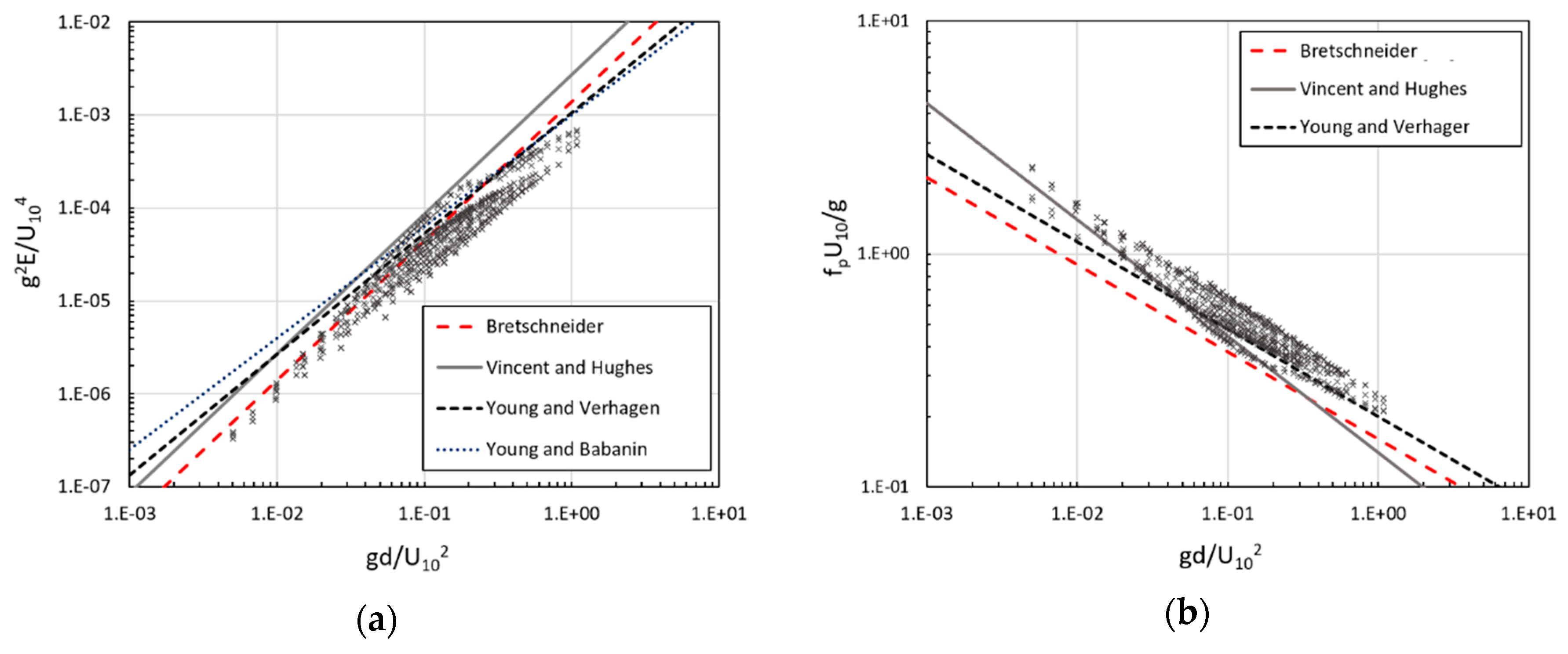
Figure 1 shows the arrangement of all the obtained points in terms of dimensionless variables with respect to the semi-empirical limits having the coefficients reported in Table 1.
As can be observed, the lines tend to define an upper and a lower bound for all the points corresponding to the wave energy and the wave peak frequency νp = 1/Tp, respectively. This result confirms that the forecasting curves (4) and (5) identify the asymptotic conditions that the generated wave field can reach for the assigned water depth and wind speed.
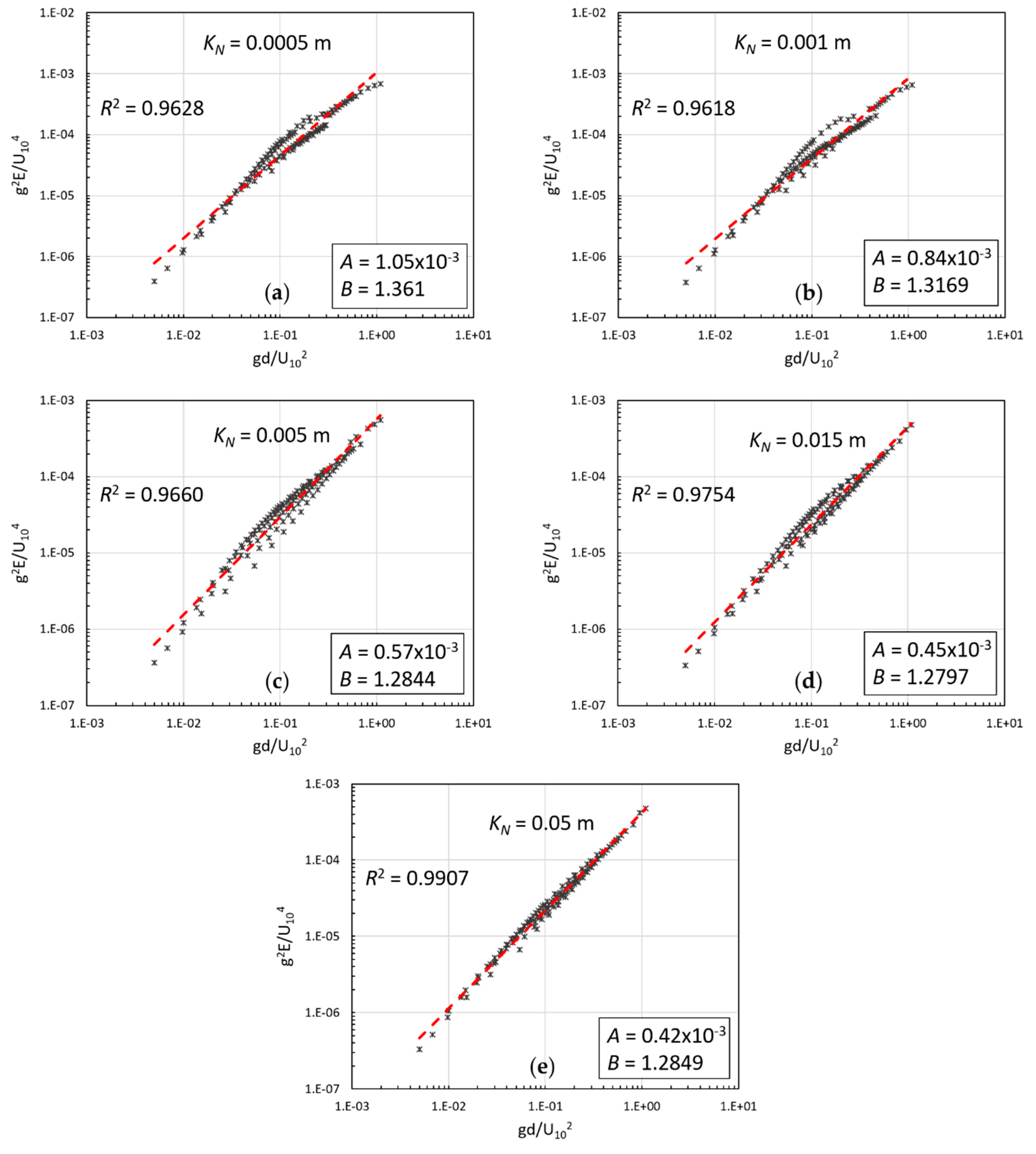
The points have been grouped according to the different bottom roughness height, with the aim of verifying whether they tend to align and, in this manner, define a particular wave field related to the bed condition. Even though there is some data scattering which in any case reduces as the roughness increases, a trend can be recognized as depicted in Figure 2. The dimensionless wave energy is represented as a function of the dimensionless depth for the KN values set to compute spectral bottom friction dissipations. The red dashed lines provide the regression of the points, and the resulting coefficients A and B entering in Equation (4) are shown in the boxes.
Parameter B defines the angular coefficient of each line and it does not change significantly between the wave field generated on different bottom roughness conditions. In particular, it remains fairly constant and equal to the value of 1.3 determined by Young and Verhagen [26], thus confirming the agreement with their results and the experimental data collected in Lake George. On the contrary, parameter A decreases progressively with the increase of KN. This means that the position of the lines in the graph and therefore the asymptotic limit that the wave energy can reach, is lowered. The maximum value of A corresponding to the minimum of KN is the same as that proposed by Young and Verhagen [26], and this further confirms the condition of the smooth flat bed of Lake George.
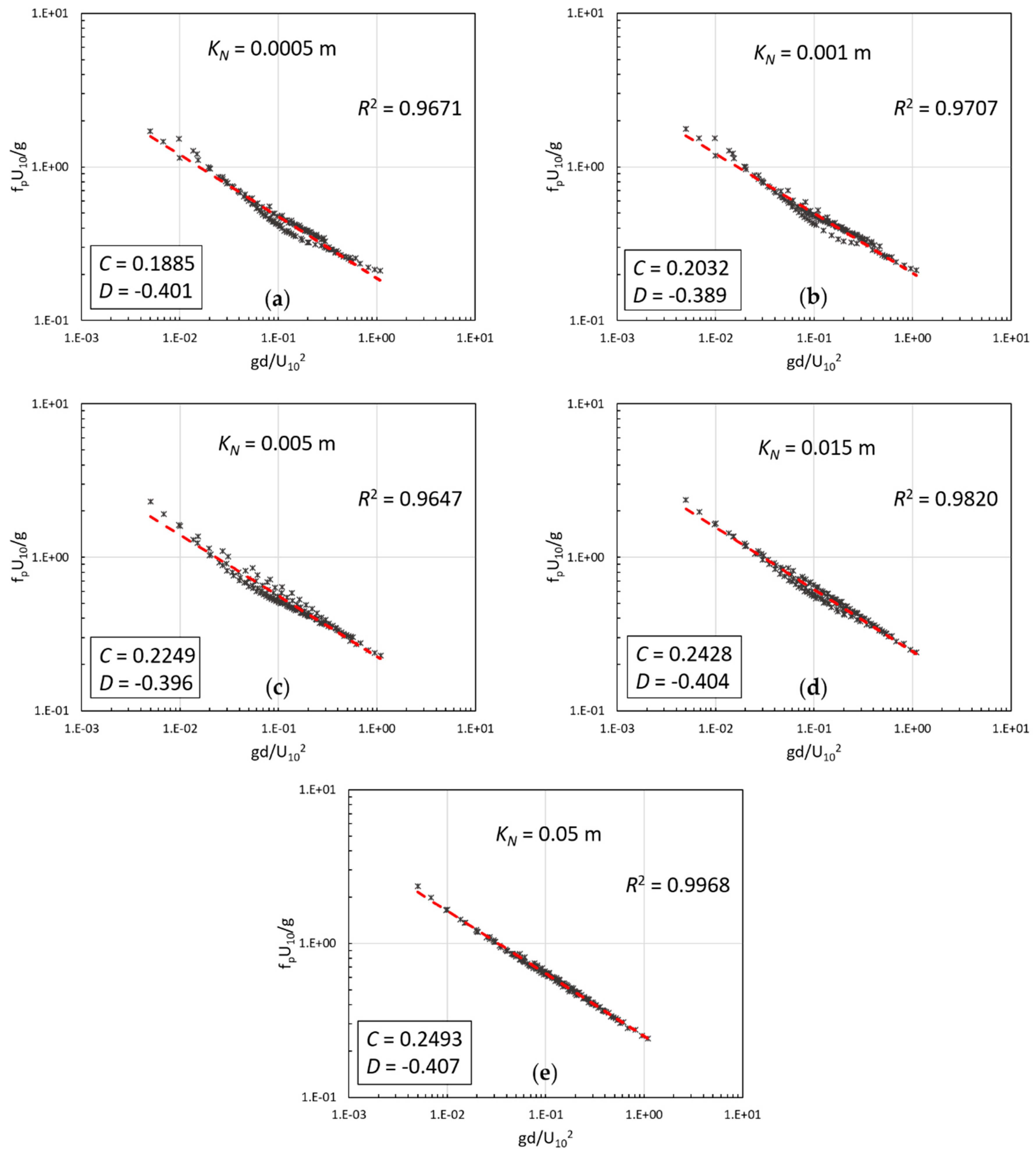
Very similar considerations can also be made on the trend of the dimensionless peak frequency reported in Figure 3.
In fact, parameter D maintains an almost constant value even if slightly lower than that of −0.375 originally proposed by Bretschneider [58] and subsequently confirmed by Young and Verhagen [26]. On the other hand, there is a dependence of the coefficient C on the bottom roughness which causes the lines to be raised in the graph with increasing KN.
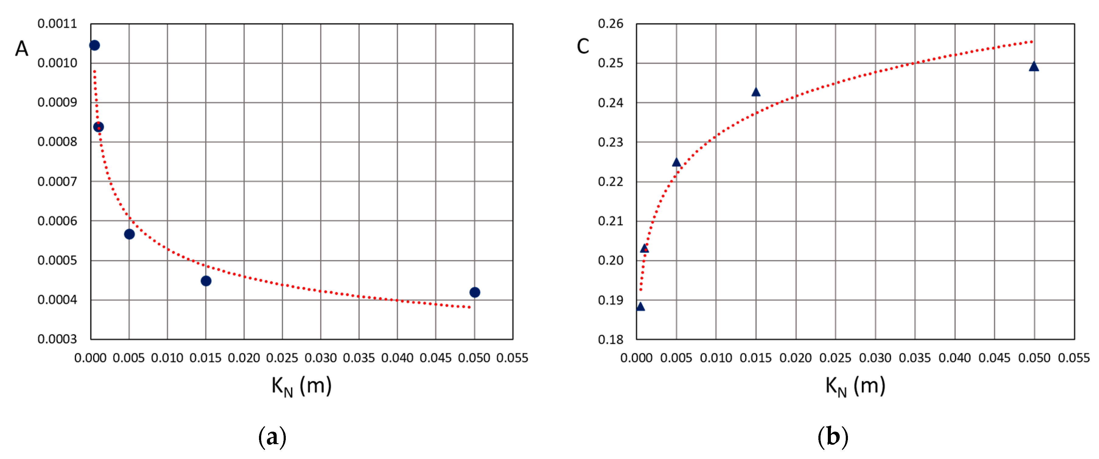
In this sense, the angular coefficients of the regression lines can be kept fixed in all the cases analyzed and equal to 1.3 for B and −0.40 for D, while the variability of the remaining parameters A and C with the bed roughness KN cannot be ignored. In order to obtain the functions that associate these coefficients to KN, the estimated values for each class of roughness have been plotted and a regression by means of the least squares method has been performed.
This analysis has led to define two polynomial curves, that can be observed in Figure 4, having the following equations respectively:
Equations (6) and (7) allow for the determination of the characteristics of the locally generated wave motion on a given depth and for an assigned wind speed, taking into account different roughness heights and therefore relative dissipation conditions of the bottom. A summary of the revised coefficients is reported in Table 2 for a more immediate comparison with those listed in Table 1.
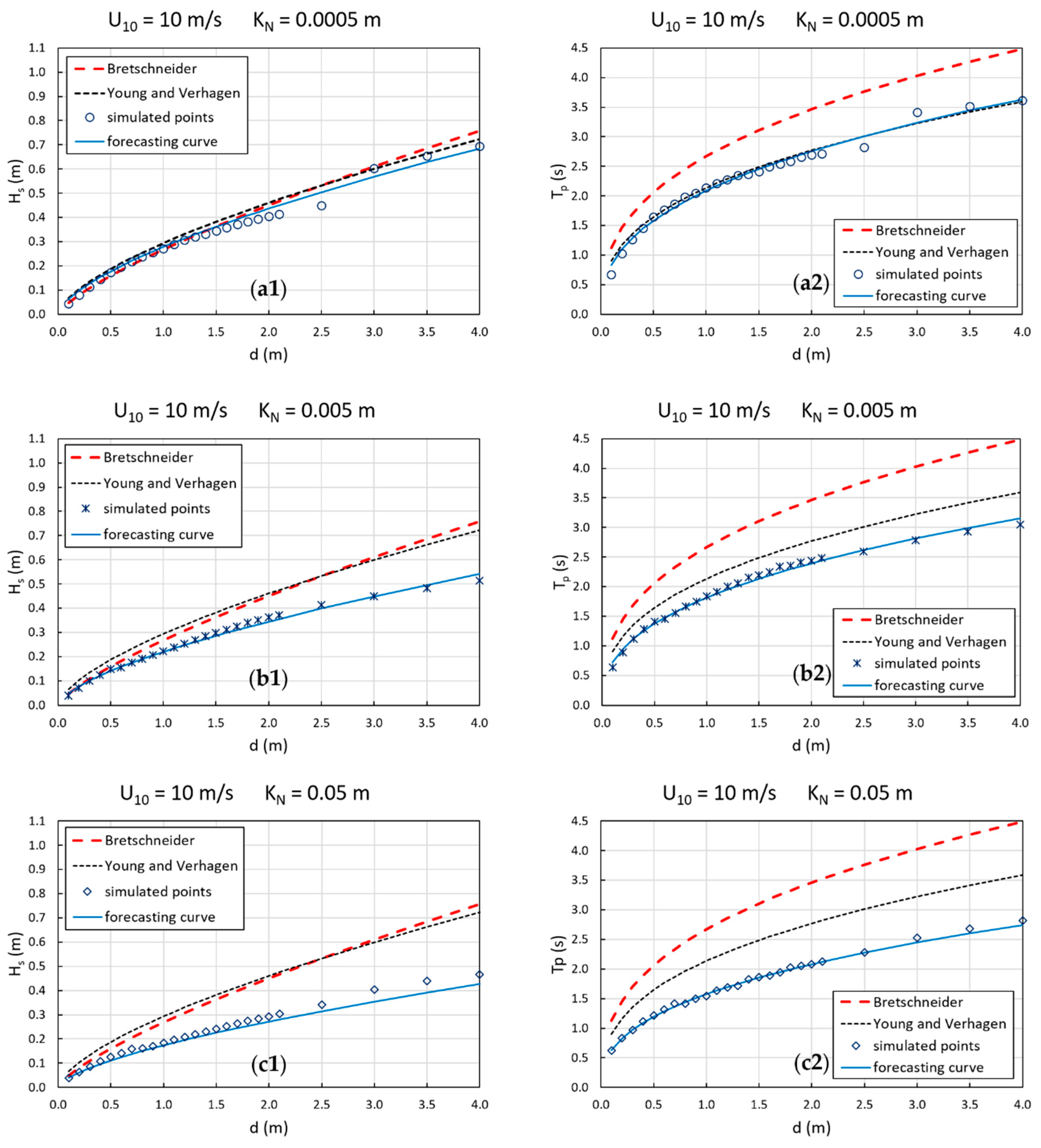
With the purpose of better understanding the differences that this approach involves with respect to the assumption of a constant friction factor, a comparative analysis based on the wave characteristics instead of on the related dimensionless variables is preferred. In fact, this choice makes it possible to analyze the trend with the depth of the wave characteristics, i.e., the significant wave height and the peak period, and to highlight where the roughness contribution is more decisive. The wind speed U10 equal to 10 m/s is taken as an example, since it is an average value in the investigated speed range.
Figure 5 presents the distribution at varying water depths of the wave fields for KN values increased progressively by an order of magnitude from the lowest value of 0.0005 m to the highest one and equal to 0.05 m. The former can be representative, as mentioned above, of a smooth and morphologically stable flat bed, for which the friction factor can be assumed as constant and equal to the commonly adopted value of 0.01 [11]. On the contrary, KN = 0.05 m can identify a very rough bottom due to the presence of ripples, vegetation, or different grain sizes. The growth curves of Bretschneider [58] and Young and Verhagen [26] are reported together with the numerically simulated points for a comparison. Both the significant wave heights, depicted in Figure 5a1–c1, and the peak periods in Figure 5a2–c2, show a great reduction if KN increases.
In particular, the wave height is lowered by 40% compared to the value predicted by assuming a not very dissipative bed. The new forecasting curve of wave energy, having coefficient A and B as reported in Table 2, is almost superimposed on those obtained by Bretschneider [58] and Young and Verhagen [26] when KN is very low, with a maximum percentage difference of 10% and 5% respectively. This confirms the more general validity of the approach. The difference between the curves of Bretschneider [58] and Young and Verhagen [26] is much more important if the peak period is considered. This outcome has been clearly pointed out by the experimental investigations in Lake George. Also in this case, Equation (5) with C and D taken according Table 2, interprets the trend of the period for the lowest value of KN well, and gives decreasing values for rougher bottoms. These results agree well with the numerical evidence performed by Graber and Madsen [41] for various conditions of bottom roughness, which clearly demonstrates the trend of decreasing energy and peak periods for rougher seabeds.
4. Application to Lake Neusiedl
A real lake has been examined to test the applicability of the forecasting curves for fully developed wave conditions on shallow depths, with the new coefficients A and C proposed by Equations (6) and (7). Experimental observations of both wind and waves are available together with the results of a complete bidimensional numerical application performed by means of a spectral model [53].
4.1. Study Site and Data Setup
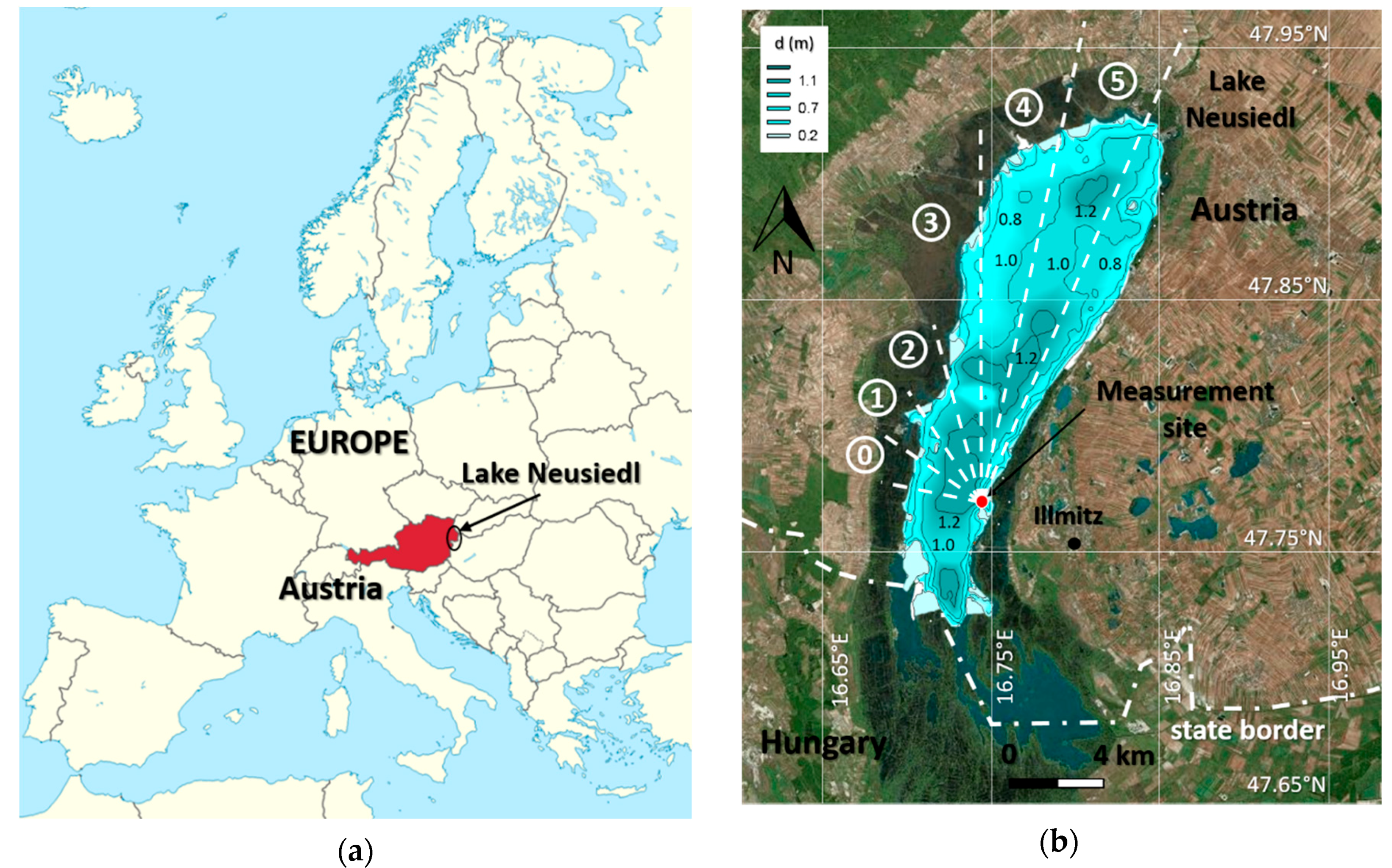
Homorodi et al. [53] have applied SWAN to Lake Neusiedl, sited between Austria and Hungary, to improve the modelling of locally generated wind waves in very shallow and confined basins.
As depicted in Figure 6, the Austrian portion of Lake Neusiedl has a quite uniform bathymetry with small depths of about 1.0–1.2 m. This particular aspect makes the context very similar to the ideal condition used in the present paper to numerically analyze and determine the growth of wind waves in shallow water. Furthermore, the extension of the lake, which stretches toward North–North East, is characterized by, at least for some wind directions and speeds, sufficiently long fetch so that the wave motion can be considered as completely developed.
In their study, Homorodi et al. [53] calibrated and validated the numerical approach with the wave data collected during two experimental campaigns conducted respectively in July and October 2005 near Illmitz, Austria. Each measurement was made for a consecutive period of about one week. The most important difference between the two stages was the direction of the dominant winds: during the first period of July it was North-West, while North and North-East during the second one. To take into account the different wave exposure and to select the conditions which lead to a fully developed wave motion, the registered wind directions provided by Homorodi et al. [53] have been grouped into six sectors as indicated in Figure 6b. A mean depth has been assigned to each sector as an average value weighted on the sector area, while the fetch has been estimated along its mean direction. In Table 3 a summary of these parameters is reported.
In the campaigns a standard wave pressure gauge was used to reconstruct the wave spectra and the relative wave parameters, in particular the significant wave height Hs and the mean wave period T01 based on the zero-order and first-order moments of the spectra. Homorodi et al. [53] compared the numerical results to both the available wave data and that estimated through the empirical growth curves of Bretschneider. The complete relations (1) and (2), that consider fetch limitation, have been adopted with the coefficients entering in Equation (3) equal to:
As the aim of this study is to apply the asymptotic form for the depth-limited Equations (4) and (5), it has been convenient to identify those records which approximately conform to this limit. These relations simplify the previous and more complete ones (1) and (2), which tend to the asymptotic form when the argument of the hyperbolic tangent depending both on fetch and depth is such as to make it close to unity.
In this sense, cases for which
have been selected, in analogy to Young and Babanin [49] who considered, for a similar purpose, a band of points within 20% of the maximum values. This approach allows us to identify the fully developed wave conditions taking into account both fetch length and depth for an assigned wind speed.
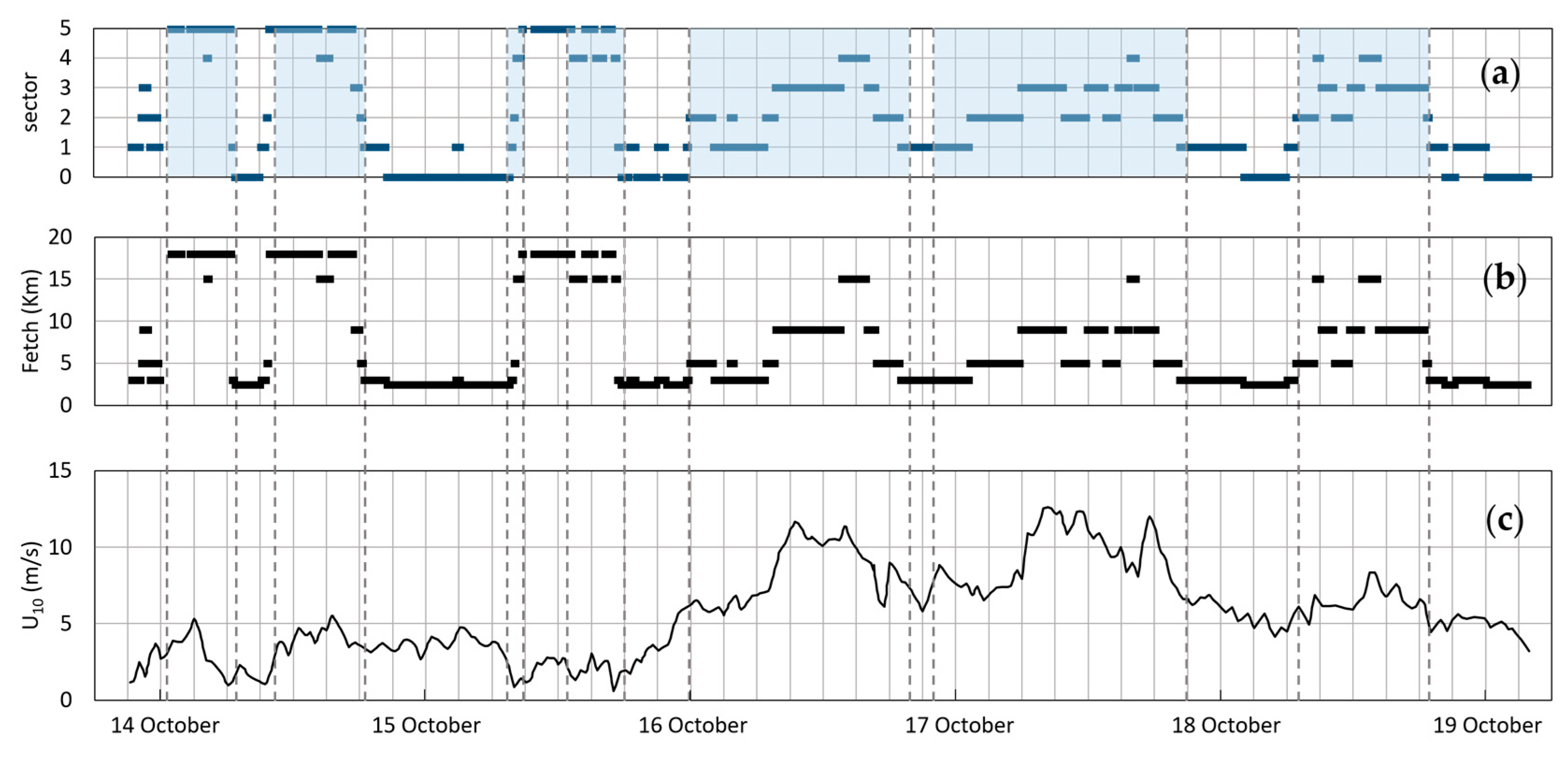
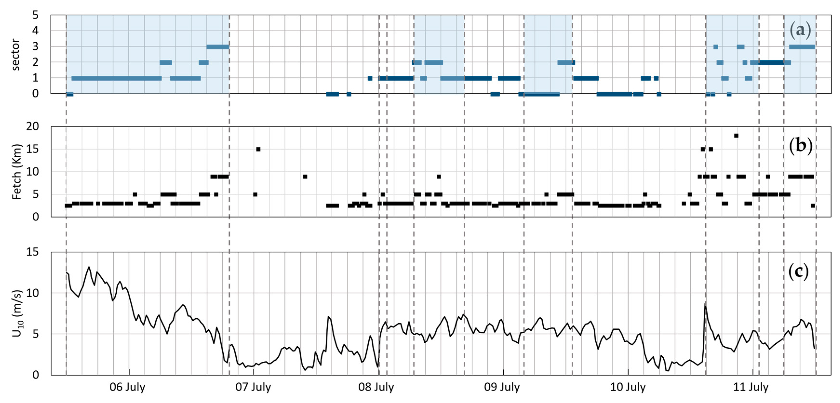
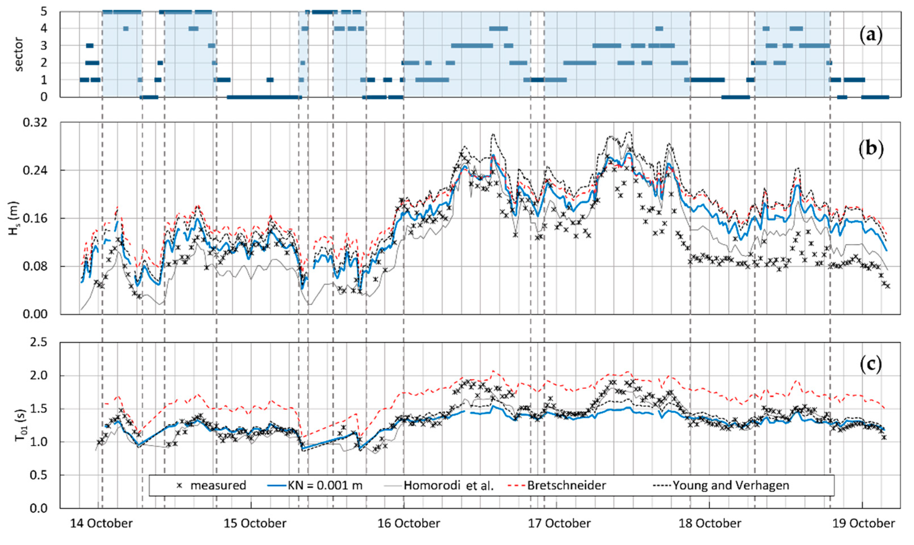
Figure 7 and Figure 8 show the measured wind data during the periods of October and July 2005 respectively. The period of October was used by Homorodi et al. [53] to calibrate SWAN and the period of July to validate the numerical approach. The blowing directions are depicted in terms of the sectors defined above, with the representative mean fetch reported in the second panel according to values in Table 3.
The colored bands highlight the selected records of wind speed, depicted in the third panel, for which Equation (10) is satisfied. As can be seen, a longer fetch is a sufficient requirement for low wind speeds, but for moderate or stronger winds even a shorter fetch can still guarantee fully developed wave motion. This outcome agrees with the recent studies of Petti et al. [33] and Pascolo et al. [11], who have found that the maximum limit of the wave growth in shallow depth is already reached on short distances of a few km, as also happens in the present case study.
To simulate bottom friction dissipations, Homorodi et al. [53] chose the formulation of Madsen et al. [40], setting a KN value of 0.001 m which produced the best agreement with the experimental data. No further details on the composition and morphology of the bed are provided, and therefore the same bottom roughness is herein taken to compute the coefficients of the depth-limited growth curves. The mean depth evaluated for each sector, together with the wind speed U10, have been used to calculate the dimensionless variable δ entering in Equations (4) and (5). Since the measured wave period is given as T01, a reduction coefficient is necessary to make a comparison with the peak period obtained by the semi-empirical relations possible. The results derived in terms of T01 and Tp from the numerical simulations described in Section 3 have been arranged in order to determine an average value of the ratio T01/Tp. This coefficient has turned out to be equal to 0.78.
4.2. Results
The results in terms of significant wave height and mean period are plotted in Figure 9 and Figure 10, respectively, for the period of October and July.
In the graphs, the values provided by the new depth-limited growth curves, defined in the present study, are compared to the measured data, the simulation results of Homorodi et al. [53] obtained by means of a complete 2D application, and those computed according to Bretschneider [58] and Young and Verhagen [26] forecasting formulations.
Focusing on the wave heights registered in the period of October, the first three days of observation, from the 14th to 17th, show a substantial agreement between the measured values and those evaluated through the new forecasting curves. On the contrary, for the following days, there is a systematic over-estimation of the wave height also through the complete 2D modelling. This discrepancy was not commented on by Homorodi et al. [53], and it could also be attributable to an instrumental error. Minor differences are found between the measured and calculated wave periods except for the highest values recorded between the 16th and 18th of October. This discrepancy can be attributed to low frequency components in the measured energy density spectra, as reported by Homorodi et al. [53] at 12:00 on the 17th of October. These components can be related to bounded long waves which are not present in the modelled energy density spectra and that lead to an overestimation of the mean period, this being calculated through the moments m0 and m1.
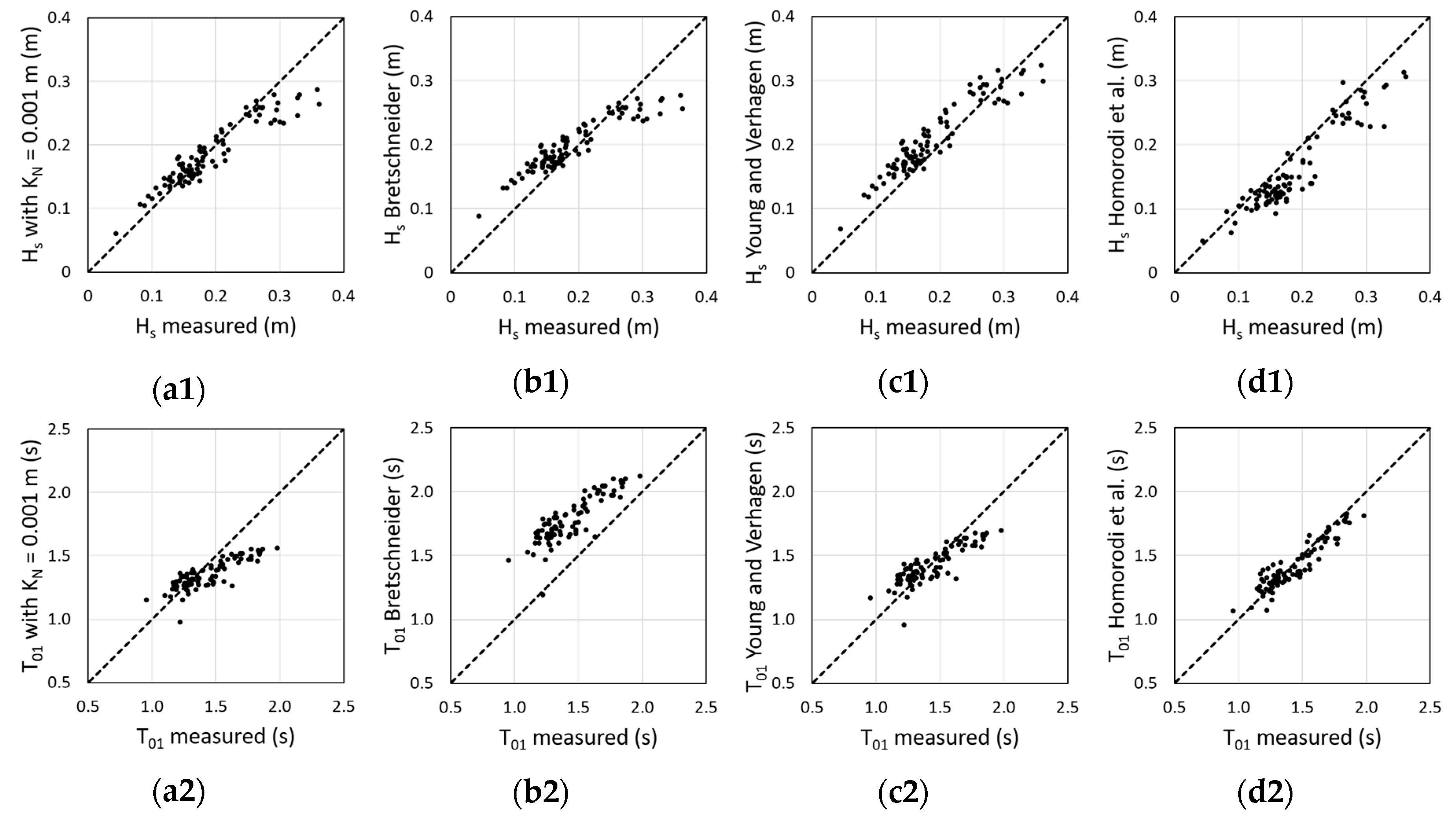
The case for July is different, for which both the wave heights and periods forecasted by the growth curves are very close to those measured.
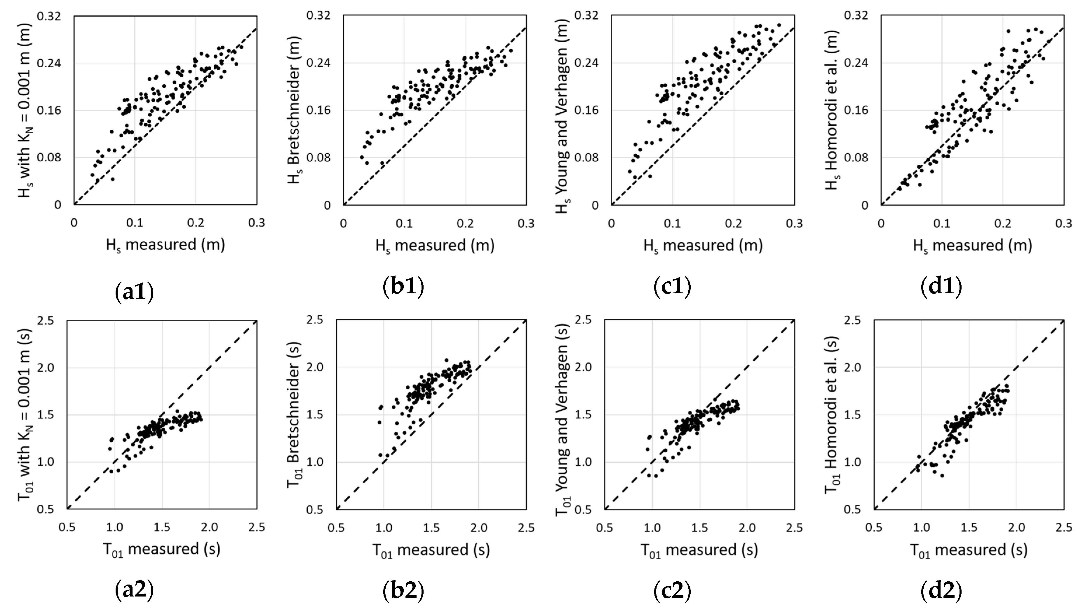
To analyze the comparison better, the selected periods which correspond to the colored bands, and therefore to a fully developed wave condition, have been grouped. The correlation graphs between the measured wave data and those calculated have been plotted, as proposed in Figure 11 for the period of October.
For the quantitative evaluation of the results, the bias parameter (BIAS), root mean square error (RMSE), scatter index (SI), and correlation coefficient (R2) have been computed as the following expressions:
where xi is the value predicted by the model or the forecasting curves and yi is the measured value, σxy the covariance, σx and σy the relative standard deviation. The obtained coefficients are reported in Table 4.
This has also been done for the July period: the correlation graphs are depicted in Figure 12 and the relative coefficients reported in Table 5.
The correlation graphs confirm that the available forecasting curves of Bretschneider [58] and Young and Verhagen [26] actually provide an upper limit to wave growth, especially for wave heights. The new curves with assigned equivalent bed roughness provide an estimate that is halfway between the aforementioned curves and the results of the 2D numerical simulation, and this is clearly highlighted by the comparison of the relative coefficients. The application of SWAN undoubtedly gives the values closest to those measured, but it requires a more detailed and complete approach.
In this sense, the proposed study has produced the expected results, given that the forecasting curves arise from the need to estimate the characteristics of wave motion through a certainly simplified but more rapid methodology.
5. Discussion and Conclusions
Numerical modelling is certainly a very valid tool to investigate wave and current hydrodynamics, especially where the complexity of the phenomena is such that it cannot be described by more simplified approaches. However, the required computational effort can be significant and a comparison with experimental and analytical results is always needed to calibrate and validate models, as in the study of Homorodi et al. described above [53].
In the absence of measured data, especially of wave motion, it is often necessary to proceed with a wave prediction system. The forecasting growth curves offer the possibility to estimate the wave characteristics more rapidly than a complete numerical approach, but still providing reliable values. In fact, the SMB (Sverdrup–Munk–Bretschneider) method [58] is widely recognized to be the most convenient and robust approach to use for computing wave heights and periods in deep water when a limited amount of data and time are available. Similarly, in shallow water contexts, the curves of Bretschneider [58] and Young and Verhagen [26] have become a widespread key reference for many applications. The domains are above all coastal areas, lagoons or lakes characterized by quite uniform bottoms and shallow depths.
The interaction with the bottom plays a crucial role in determining the wave components, but there is still an ongoing debate as to how the roughness can be involved in the forecasting equations. This study suggests the possibility of making the equations dependent on the bed roughness, while remaining consistent with those of Bretschneider [58] and Young and Verhagen [26]. At the same time, some important intuitions on the friction influence, as for example the outcomes determined in the numerical field by Graber and Madsen [41], are considered.
This first step has been carried out by starting from the simpler asymptotic form of the growth curves, corresponding to a fully developed wave condition, which is therefore not affected by the fetch limitation. The proposed approach is able to adequately address the question of estimating the main wave characteristics if the wind speed, the depth, and the equivalent bottom roughness are assigned. The coefficients entering the forecasting Equations (4) and (5) have been reformulated as a function of the KN value, as indicated in Table 2, leading to a new set of relations.
The curves depicted as examples in Figure 5 seem to confirm the validity of the method. In fact, the lowest value of KN, i.e., 0.0005 m, returns the limits of Young and Verhagen [26] exactly both for the wave heights and peak periods. This value is representative of a friction factor equal to 0.01, for which bottom resistance is beginning to show its influence, as already found by Graber and Madsen [41]. Moreover, the same value is also compatible with both that considered by Bretschneider [58] and the description of the bottom conditions of Lake George, very smooth and with no bedforms, where Young and Verhagen [26] carried out their important experimental measurements. On the contrary, the increase in roughness, and therefore of the friction factor, causes the substantial reduction of Hs and Tp. The new curves also show the good adaptability to scatter points determined numerically with SWAN, further validating the results.
The application of the new equations system to the real case study satisfies the expectations for a better estimate of the wave field generated in shallow and confined basins, compared to Bretschneider [58] and Young and Verhagen [26]. Furthermore, the forecasted values of wave heights and periods, taking into account an equivalent roughness of 0.001 m, are very close to those computed by means of a complete 2D numerical modelling [53]. The domain is very similar to the test case involved in the preliminary numerical investigations and also to Lake George, with a very small depth of about 1.0 m.
The quantitative analyses of the results have been performed by selecting the conditions of wind speed and depth which ensure a fully developed wave field. The criterion established and formalized in Equation (10) has highlighted that in depth-limited conditions, the wave motion becomes independent from the fetch length over shorter distances of some km, if the wind speed is greater than about 5 m/s. This outcome agrees with the Young and Babanin study [49], which collected fully developed conditions over a maximum fetch length of about 7 km for a water depth ranging from 0.4 m to 1.5 m and wind speeds of no less than 6 m/s. Petti et al. [33] also found that the maximum wave heights and periods are reached over a distance of 3–4 km, inside the microtidal basin of a shallow lagoon. In this case, the bed roughness can be greater than 0.001 m, since the composition of the sediments can vary and ripples or irregularities can arise, leading to an increase of the friction factor.
The differences between the values derived from the Young and Verhagen formulation and those computed by the new set of equations are not so important with KN values lower than 0.001 m, also given the very shallow water. However, these initial results encourage future developments of this study, providing for the application of the new curves to coastal or lagoon contexts, with more irregular seabeds, and the necessary comparison with observed wave data.
Author Contributions
M.P., S.P., and S.B. contributed equally to this work.
Funding
This research received no external funding.
Conflicts of Interest
The authors declare no conflict of interest.
References
- Fredsøe, J.; Deigaard, R. Mechanics of Coastal Sediment Transport; Advanced Series on Ocean Engineering; World Scientific: Singapore, 1992; Volume 3, p. 369. [Google Scholar]
- Nielsen, P. Coastal and Estuarine Processes; Advanced Series on Ocean Engineering; World Scientific: Singapore, 2009; Volume 29, p. 345. [Google Scholar]
- Fagherazzi, S.; Palermo, C.; Rulli, M.C.; Carniello, L.; Defina, A. Wind waves in shallow microtidal basins and the dynamic equilibrium of tidal flats. J. Geophys. Res. 2007, 112, F02024. [Google Scholar] [CrossRef]
- Le Hir, P.; Roberts, W.; Cazaillet, O.; Christie, M.; Bassoullet, P.; Bacher, C. Characterization of intertidal flat hydrodynamics. Cont. Shelf Res. 2000, 20, 1433–1459. [Google Scholar] [CrossRef] [Green Version]
- Friedrichs, C.L. Tidal flat morphodynamics: A synthesis. In Treatise on Estuarine and Coastal Science; Estuarine and Coastal Geology and Geomorphology; Hansom, J.D., Fleming, B.W., Eds.; Elsevier: Amsterdam, The Netherlands, 2011; Volume 3, pp. 137–170. [Google Scholar]
- Green, M.O. Very small waves and associated sediment resuspension on an estuarine intertidal flat. Estuar. Coast. Shelf Sci. 2011, 93, 449–459. [Google Scholar] [CrossRef]
- Green, M.O.; Coco, G. Review of wave-driven sediment resuspension and transport in estuaries. Rev. Geophys. 2014, 52, 77–117. [Google Scholar] [CrossRef]
- Shi, B.; Cooper, J.R.; Li, J.; Yang, Y.; Yang, S.L.; Luo, F.; Yu, Z.; Wang, Y.P. Hydrodynamics, erosion and accretion of intertidal mudflats in extremely shallow waters. J. Hydrol. 2019, 573, 31–39. [Google Scholar] [CrossRef]
- Sheng, Y.P.; Lick, W. The transport and resuspension of sediments in a shallow lake. J. Geophys. Res. 1979, 84, 1809–1826. [Google Scholar] [CrossRef]
- Carper, G.L.; Bachmann, R.W. Wind Resuspension of Sediments in a Prairie Lake. Can. J. Fish. Aquat. Sci. 1984, 41, 1763–1767. [Google Scholar] [CrossRef]
- Pascolo, S.; Petti, M.; Bosa, S. On the Wave Bottom Shear Stress in Shallow Depths: The Role of Wave Period and Bed Roughness. Water 2018, 10, 1348. [Google Scholar] [CrossRef]
- Petti, M.; Pascolo, S.; Bosa, S.; Bezzi, A.; Fontolan, G. Tidal Flats Morphodynamics: A new Conceptual Model to Predict Their Evolution over a Medium-Long Period. Water 2019, 11, 1176. [Google Scholar] [CrossRef]
- Chao, X.; Jia, Y.; Shields, F.D.; Wang, S.S.Y.; Cooper, C.M. Three-dimensional numerical modeling of cohesive sediment transport and wind wave impact in a shallow oxbow lake. Adv. Water Resour. 2008, 31, 1004–1014. [Google Scholar] [CrossRef]
- Jin, K.R.; Wang, K.H. Wind generated waves in Lake Okeechobee. JAWRA J. Am. Water Resour. Assoc. 2007, 34, 1099–1108. [Google Scholar] [CrossRef]
- Carniello, L.; Defina, A.; D’Alpaos, L. Morphological evolution of the Venice lagoon: Evidence from the past and trend for the future. J. Geophys. Res. 2009, 114, F04002. [Google Scholar] [CrossRef]
- Shi, B.W.; Yang, S.L.; Wang, Y.P.; Bouma, T.J.; Zhu, Q. Relating accretion and erosion at an exposed tidal wetland to the bottom shear stress of combined current–wave action. Geomorphology 2012, 138, 380–389. [Google Scholar] [CrossRef]
- Zhu, Q.; van Prooijen, B.C.; Wang, Z.B.; Yang, S.L. Bed-level changes on intertidal wetland in response to waves and tides: A case study from the Yangtze River Delta. Mar. Geol. 2017, 385, 160–172. [Google Scholar] [CrossRef]
- Bachmann, R.W.; Hoyer, M.V.; Canfield, D.E., Jr. The Potential for Wave Disturbance in Shallow Florida Lakes. Lake Reserv. Manag. 2000, 16, 281–291. [Google Scholar] [CrossRef]
- Kirby, R. Practical implications of tidal flat shape. Cont. Shelf Res. 2000, 20, 1061–1077. [Google Scholar] [CrossRef]
- Callaghan, D.P.; Bouma, T.J.; Klaassen, P.; van der Wal, D.; Stive, M.J.F.; Herman, P.M.J. Hydrodynamic forcing on salt-marsh development: Distinguishing the relative importance of waves and tidal flows. Estuar. Coast. Shelf Sci. 2010, 89, 73–88. [Google Scholar] [CrossRef]
- Hu, Z.; Wang, Z.B.; Zitman, T.J.; Stive, M.J.F.; Bouma, T.J. Predicting long-term and short-term tidal flat morphodynamics using a dynamic equilibrium theory. J. Geophys. Res. Earth Surf. 2015, 120, 1803–1823. [Google Scholar] [CrossRef] [Green Version]
- Shi, B.; Cooper, J.R.; Pratolongo, P.D.; Gao, S.; Bouma, T.J.; Li, G.; Li, C.; Yang, S.L.; Wang, Y.P. Erosion and accretion on a mudflat: The importance of very shallow-water effects. J. Geophys. Res. Ocean. 2017, 122, 9476–9499. [Google Scholar] [CrossRef]
- Jalil, A.; Li, Y.; Zhang, K.; Gao, X.; Wang, W.; Sarwar Khan, H.O.; Pan, B.; Ali, S.; Acharya, K. Wind-induced hydrodynamic changes impact on sediment resuspension for large, shallow Lake Taihu, China. Int. J. Sediment Res. 2019, 34, 205–215. [Google Scholar] [CrossRef]
- Bretschneider, C.L.; Reid, R.O. Change in Wave Height Due to Bottom Friction, Percolation and Refraction; Tech. Memo No. 45; Beach Erosion Board Engineer Research and Development Center (U.S.): Boston, MA, USA, 1954. [Google Scholar]
- Bretschneider, C.L. Generation of Wind Waves in Shallow Water; Beach Erosion Board; Tech. Memo No. 51; Beach Erosion Board Engineer Research and Development Center (U.S.): Boston, MA, USA, 1954. [Google Scholar]
- Young, I.R.; Verhagen, L.A. The growth of fetch limited waves in water of finite depth. 1. Total energy and peak frequency. Coast. Eng. 1996, 29, 47–78. [Google Scholar] [CrossRef]
- Umgiesser, G.; Sclavo, M.; Carniel, S.; Bergamasco, A. Exploring the bottom shear stress variability in the Venice Lagoon. J. Mar. Syst. 2004, 51, 161–178. [Google Scholar] [CrossRef]
- Carniello, L.; Silvestri, S.; Marani, M.; D’Alpaos, A.; Volpe, V.; Defina, A. Sediment dynamics in shallow tidal basins: In situ observations, satellite retrievals, and numerical modeling in the Venice Lagoon. J. Geophys. Res. Earth Surf. 2014, 119, 802–815. [Google Scholar] [CrossRef] [Green Version]
- Cappucci, S.; Amos, C.L.; Hosoe, T.; Umgiesser, G. SLIM: A numerical model to evaluate the factors controlling the evolution of intertidal mudflats in Venice Lagoon, Italy. J. Mar. Syst. 2004, 51, 257–280. [Google Scholar] [CrossRef]
- Fagherazzi, S.; Wiberg, P.L. Importance of wind conditions, fetch, and water levels on wave-generated shear stresses in shallow intertidal basins. J. Geophys. Res. 2009, 114, F03022. [Google Scholar] [CrossRef]
- Carniello, L.; Defina, A.; D’Alpaos, L. Modeling sand-mud transport induced by tidal currents and wind waves in shallow microtidal basins: Application to the Venice Lagoon (Italy). Estuar. Coast. Shelf Sci. 2012, 102, 105–115. [Google Scholar] [CrossRef]
- Zhou, Z.; Coco, G.; van der Wegen, M.; Gong, Z.; Zhang, C.; Townend, I. Modeling sorting dynamics of cohesive and non-cohesive sediments on intertidal flats under the effect of tides and wind waves. Cont. Shelf Res. 2015, 104, 76–91. [Google Scholar] [CrossRef]
- Petti, M.; Bosa, S.; Pascolo, S. Lagoon Sediment Dynamics: A Coupled Model to Study a Medium-Term Silting of Tidal Channels. Water 2018, 10, 569. [Google Scholar] [CrossRef]
- Gorman, R.M.; Neilson, C.G. Modelling shallow water wave generation and transformation in an intertidal estuary. Coast. Eng. 1999, 36, 197–217. [Google Scholar] [CrossRef]
- Petti, M.; Bosa, S.; Pascolo, S.; Uliana, E. Marano and Grado Lagoon: Narrowing of the Lignano Inlet. IOP Conf. Ser. Mater. Sci. Eng. 2019, 603, 032066. [Google Scholar] [CrossRef]
- Petti, M.; Pascolo, S.; Bosa, S.; Uliana, E.; Faggiani, M. Sea defences design in the vicinity of a river mouth: The case study of Lignano Riviera and Pineta. IOP Conf. Ser. Mater. Sci. Eng. 2019, 603, 032067. [Google Scholar] [CrossRef]
- Holthuijsen, L.H.; Booij, N.; Herbers, T.H.C. A prediction model for stationary, short-crested waves in shallow water with ambient currents. Coast. Eng. 1989, 13, 23–54. [Google Scholar] [CrossRef]
- Booij, N.; Ris, R.C.; Holthuijsen, L.H. A third-generation wave model for coastal regions, Part I, Model description and validation. J. Geophys. Res. 1999, 104, 7649–7666. [Google Scholar] [CrossRef]
- Shemdin, O.H.; Hsiao, S.V.; Carlson, H.E.; Hasselmann, K.; Schulze, K. Mechanisms of wave transformation in finite-depth water. J. Geophys. Res. 1980, 85, 5012–5018. [Google Scholar] [CrossRef] [Green Version]
- Madsen, O.S.; Poon, Y.-K.; Graber, H.C. Spectral wave attenuation by bottom friction: Theory. In Proceedings of the 21th International Conference Coastal Engineering, ASCE, Costa del Sol-Malaga, Spain, 20–25 June 1988; pp. 492–504. [Google Scholar]
- Graber, H.C.; Madsen, O.S. A Finite-Depth Wind-Wave Model. Part I: Model Description. J. Phys. Oceanogr. 1988, 18, 1465–1483. [Google Scholar] [CrossRef] [Green Version]
- Young, I.R.; Verhagen, L.A. The growth of fetch limited waves in water of finite depth. Part 2. Spectral evolution. Coast. Eng. 1996, 29, 79–99. [Google Scholar] [CrossRef]
- Zijlema, M.; van Vledder, G.P.; Holthuijsen, L.H. Bottom friction and wind drag for wave models. Coast. Eng. 2012, 65, 19–26. [Google Scholar] [CrossRef]
- Vincent, C.L.; Hughes, S.A. Wind Wave Growth in Shallow Water. J. Waterw. Port Coast. Ocean Eng. 1985, 111, 765–770. [Google Scholar] [CrossRef]
- Bouws, E.; Günther, H.; Rosenthal, W.; Vincent, C.L. Similarity of the wind wave spectrum in finite depth water: 1. Spectral form. J. Geophys. Res. 1985, 90, 975–986. [Google Scholar] [CrossRef]
- Hasselmann, K. On the non-linear energy transfer in a gravity-wave spectrum Part 1. General theory. J. Fluid Mech. 1962, 12, 481–500. [Google Scholar] [CrossRef]
- Ijima, T.; Tang, F.L.W. Numerical Calculation of Wind Waves in Shallow Water. Coast. Eng. 1966, 38–49. [Google Scholar] [CrossRef]
- Young, I.R.; Banner, M.L.; Donelan, M.A.; McCormick, C.; Babanin, A.V.; Melville, W.K.; Veron, F. An Integrated System for the Study of Wind-Wave Source Terms in Finite-Depth Water. J. Atmos. Ocean. Technol. 2005, 22, 814–831. [Google Scholar] [CrossRef]
- Young, I.R.; Babanin, A.V. The form of the asymptotic depth-limited wind wave frequency spectrum. J. Geophys. Res. 2006, 111, C06031. [Google Scholar] [CrossRef]
- Breugem, W.A.; Holthuijsen, L.H. Generalized Shallow Water Wave Growth from Lake George. J. Waterw. PortCoast. Ocean Eng. 2007, 133, 173–182. [Google Scholar] [CrossRef]
- Mariotti, G.; Fagherazzi, S. A two-point dynamic model for the coupled evolution of channels and tidal flats. J. Geophys. Res. Earth Surf. 2013, 118, 1387–1399. [Google Scholar] [CrossRef]
- Mariotti, G.; Fagherazzi, S. Wind waves on a mudflat: The influence of fetch and depth on bed shear stresses. Cont. Shelf Res. 2013, 60, S99–S110. [Google Scholar] [CrossRef]
- Homorodi, K.; Józsa, J.; Krámer, T. On the 2D modelling aspects of wind-induced waves in shallow, fetch-limited lakes. Period. Polytech. Civ. Eng. 2012, 56, 127–140. [Google Scholar] [CrossRef]
- Soulsby, R.L. Dynamics of Marine Sands: A Manual for Practical Applications; Thomas Telford Publications: London, UK, 1997; 249p. [Google Scholar]
- Whitehouse, R.J.S.; Soulsby, R.L.; Roberts, W.; Mitchener, H.J. Dynamics of Estuarine Muds; Technical Report; Thomas Telford: London, UK, 2000. [Google Scholar]
- Bretschneider, C.L. Revisions in wave forecasting: Deep and shallow water. Coast. Eng. Proc. 1957, 1, 30–67. [Google Scholar] [CrossRef]
- Pascolo, S.; Petti, M.; Bosa, S. Wave–Current Interaction: A 2DH Model for Turbulent Jet and Bottom-Friction Dissipation. Water 2018, 10, 392. [Google Scholar] [CrossRef]
- CERC (U.S. Army Coastal Engineering Research Center). Shore Protection Manual; U.S. Army Coastal Engineering Research Center: Washington, DC, USA, 1973; Volume 1. [Google Scholar]
Figure 1.
Scatter points numerically obtained with generation process in shallow depths in terms of dimensionless variables: (a) the wave energy, and (b) the peak frequency as functions of water depth. The lines represent the semi-empirical Equations (4) and (5) according to the authors listed in Table 1.

Figure 2.
Dimensionless wave energy grouped by different bottom roughness values: (a) KN = 0.0005 m; (b) KN = 0.0001 m; (c) KN = 0.005 m; (d) KN = 0.015 m; (e) KN = 0.05 m. Red dashed lines are regression curves obtained by means of the least squares method. Correlation coefficients R2 of each linear regression are indicated on each plot. The relative coefficients A and B entering in Equation (4) are shown in the boxes.

Figure 3.
Dimensionless wave peak frequency grouped by different bottom roughness values: (a) KN = 0.0005 m; (b) KN = 0.0001 m; (c) KN = 0.005 m; (d) KN = 0.015 m; (e) KN = 0.05 m. Red dashed lines are regression curves obtained by means of the least squares method. Correlation coefficients R2 of each linear regression are indicated on each plot. The relative coefficients C and D entering in Equation (5) are shown in the boxes.

Figure 4.
Values of: (a) the coefficient A entering in Equation (4) and (b) the coefficient C entering in Equation (5), as a function of the equivalent bottom roughness. The dotted lines are the relative regression curves by means of the least squares method.
Figure 4.
Values of: (a) the coefficient A entering in Equation (4) and (b) the coefficient C entering in Equation (5), as a function of the equivalent bottom roughness. The dotted lines are the relative regression curves by means of the least squares method.

Figure 5.
Distribution at varying water depths of the wave field generated by a wind speed U10 of 10 m/s for different KN values: (a1–c1) the significant wave height and (a2–c2) the wave peak period. The red and black dashed lines refer to the growth curves predicted by Bretschneider [58] and Young and Verhagen [26] respectively. The points are the results obtained by means of the spectral model.

Figure 6.
Lake Neusiedl depicted (a) in the European context, and (b) with the contour of bathymetry of the Austrian portion. The dashed white lines define the sectors of the blowing wind data collected by the anemometer placed in the measurement site shown by the arrow. The sectors are numbered as indicated by the circles.

Figure 7.
Wind data measured during the campaign of October 2005 [53]: (a) sectors of blowing winds; (b) the relative mean fetch according to the values in Table 3; (c) the wind speeds. The colored bands limited by the dashed lines correspond to the conditions of fully developed wave motion which satisfy relation (10).

Figure 8.
Wind data measured during the campaign of July 2005 [53]: (a) sectors of blowing winds; (b) the relative mean fetch according to the values in Table 3; (c) the wind speeds. The colored bands limited by the dashed lines correspond to the conditions of fully developed wave motion which satisfy relation (10).

Figure 9.
October 2005: (a) sectors of blowing winds with the selected colored records that correspond to fully developed wave conditions; (b) significant wave heights; (c) mean wave periods. Asterisks indicate measured data; the bold blue line indicates the results given by the growth curve with KN of 0.001 m, the dashed red line the forecasting values obtained with the Bretschneider formula, and the black dotted line those obtained with Young and Verhagen formula.

Figure 10.
July 2005: (a) sectors of blowing winds with the selected colored records that correspond to fully developed wave conditions; (b) significant wave heights; (c) mean wave periods. Asterisks indicate measured data; the bold blue line indicates the results given by the growth curve with KN of 0.001 m, the dashed red line the forecasting values obtained with the Bretschneider formula, and the black dotted line those obtained with Young and Verhagen formula.

Figure 11.
Correlation between the fully developed wave data measured in October 2005 and that given by: (a1-2) the growth curve with KN = 0.001 m; (b1-2) Bretschneider [58] formulation; (c1-2) Young and Verhagen [26] formulation; (d1-2) Homorodi et al. [53] bidimensional (2D) spectral application.

Figure 12.
Correlation between the fully developed wave data measured in July 2005 and that given by: (a1-2) the growth curve with KN = 0.001 m; (b1-2) Bretschneider [58] formulation; (c1-2) Young and Verhagen [26] formulation; (d1-2) Homorodi et al. [53] bidimensional (2D) spectral application.


Table 1.
Constant values of the coefficients entering in the limit Equations (4) and (5), according to different authors.
Table 1.
Constant values of the coefficients entering in the limit Equations (4) and (5), according to different authors.
| Authors | A | B | C | D |
|---|---|---|---|---|
| Bretschneider [58] | 1.4 × 10⁻³ | 1.5 | 0.16 | −0.375 |
| Vincent and Hughes [44] | 2.7 × 10⁻³ | 1.5 | 0.14 | −0.5 |
| Young and Verhagen [26] | 1.06 × 10⁻³ | 1.3 | 0.20 | −0.375 |
| Young and Babanin [49] | 1.0 × 10⁻³ | 1.2 | - | - |
Table 2.
Revised coefficients entering in the limit Equations (4) and (5) as functions of KN.
| A | B | C | D |
|---|---|---|---|
| 0.0002 KN−0.205 | 1.3 | 0.307 KN0.061 | −0.40 |
Table 3.
Sectors of blowing winds: the second column reports the directions that limit each sector; the mean depth is calculated as an average value weighted on the sector area; the fetch is taken along the mean direction of the sector.
Table 3.
Sectors of blowing winds: the second column reports the directions that limit each sector; the mean depth is calculated as an average value weighted on the sector area; the fetch is taken along the mean direction of the sector.
| Sector | Directions | Mean Depth (m) | Fetch (Km) |
|---|---|---|---|
| 0 | 290° N–310° N | 0.82 | 2.5 |
| 1 | 310° N–330° N | 0.88 | 3 |
| 2 | 330° N–345° N | 0.84 | 5 |
| 3 | 345° N–360° N | 0.79 | 9 |
| 4 | 0° N–12° N | 0.91 | 15 |
| 5 | 12° N–24° N | 0.90 | 18 |
Table 4.
Coefficients related to wave heights and periods measured and computed referring to the October period. BIAS, bias parameter; RMSE, root mean square error; SI, scatter index; R2,correlation coefficient.
Table 4.
Coefficients related to wave heights and periods measured and computed referring to the October period. BIAS, bias parameter; RMSE, root mean square error; SI, scatter index; R2,correlation coefficient.
| Statistical Coefficients | KN = 0.001 m | Bretschneider [58] | Young and Verhagen [26] | Homorodi et al. [53] | ||||
|---|---|---|---|---|---|---|---|---|
| Hs | T01 | Hs | T01 | Hs | T01 | Hs | T01 | |
| BIAS | 0.034 m | −0.140 s | 0.047 m | 0.286 s | 0.058 m | −0.069 s | 0.014 m | −0.062 s |
| RMS | 0.044 m | 0.204 s | 0.058 m | 0.312 s | 0.065 m | 0.147 s | 0.035 m | 0.116 s |
| SI | 29.567 | 13.738 | 38.661 | 21.010 | 43.486 | 9.911 | 23.305 | 7.788 |
| R2 | 0.881 | 0.817 | 0.861 | 0.837 | 0.881 | 0.837 | 0.878 | 0.906 |
Table 5.
Coefficients related to wave heights and periods measured and computed referring to the July period.
Table 5.
Coefficients related to wave heights and periods measured and computed referring to the July period.
| Statistical Coefficients | KN = 0.001 m | Bretschneider [58] | Young and Verhagen [26] | Homorodi et al. [53] | ||||
|---|---|---|---|---|---|---|---|---|
| Hs | T01 | Hs | T01 | Hs | T01 | Hs | T01 | |
| BIAS | −0.005 m | −0.079 s | 0.009 m | 0.350 s | 0.019 m | −0.006 s | −0.028 m | −0.009 s |
| RMS | 0.027 m | 0.158 s | 0.034 m | 0.365 s | 0.030 m | 0.121 s | 0.036 m | 0.083 s |
| SI | 14.250 | 11.014 | 18.068 | 25.470 | 16.070 | 8.418 | 18.982 | 5.772 |
| R2 | 0.941 | 0.847 | 0.933 | 0.857 | 0.941 | 0.857 | 0.938 | 0.930 |
© 2019 by the authors. Licensee MDPI, Basel, Switzerland. This article is an open access article distributed under the terms and conditions of the Creative Commons Attribution (CC BY) license (http://creativecommons.org/licenses/by/4.0/).
Share and Cite
MDPI and ACS Style
Pascolo, S.; Petti, M.; Bosa, S. Wave Forecasting in Shallow Water: A New Set of Growth Curves Depending on Bed Roughness. Water 2019, 11, 2313. https://doi.org/10.3390/w11112313
AMA Style
Pascolo S, Petti M, Bosa S. Wave Forecasting in Shallow Water: A New Set of Growth Curves Depending on Bed Roughness. Water. 2019; 11(11):2313. https://doi.org/10.3390/w11112313
Chicago/Turabian StylePascolo, Sara, Marco Petti, and Silvia Bosa. 2019. "Wave Forecasting in Shallow Water: A New Set of Growth Curves Depending on Bed Roughness" Water 11, no. 11: 2313. https://doi.org/10.3390/w11112313
Note that from the first issue of 2016, this journal uses article numbers instead of page numbers. See further details here.