Article

Streambed Flux Measurement Informed by Distributed Temperature Sensing Leads to a Significantly Different Characterization of Groundwater Discharge

1
Conservation and Survey Division, School of Natural Resources, University of Nebraska-Lincoln, Lincoln, NE 68583, USA
2
Department of Biological Systems Engineering, University of Nebraska-Lincoln, Lincoln, NE 68583, USA
3
U.S. Geological Survey, Hydrogeophysics Branch, 11 Sherman Place, Unit 5015, Storrs, CT 06269, USA
4
Earth and Atmospheric Sciences, University of Nebraska-Lincoln, Lincoln, NE 68588, USA
*
Author to whom correspondence should be addressed.
Water 2019, 11(11), 2312; https://doi.org/10.3390/w11112312
Submission received: 26 September 2019 / Revised: 28 October 2019 / Accepted: 29 October 2019 / Published: 5 November 2019
(This article belongs to the Special Issue Groundwater-Surface Water Interactions)

Abstract

:
Groundwater discharge though streambeds is often focused toward discrete zones, indicating that preliminary reconnaissance may be useful for capturing the full spectrum of groundwater discharge rates using point-scale quantitative methods. However, many direct-contact reconnaissance techniques can be time-consuming, and remote sensing (e.g., thermal infrared) typically does not penetrate the water column to locate submerged seepages. In this study, we tested whether dozens of groundwater discharge measurements made at “uninformed” (i.e., selected without knowledge on high-resolution temperature variations at the streambed) point locations along a reach would yield significantly different Darcy-based groundwater discharge rates when compared with “informed” measurements, focused at streambed thermal anomalies that were identified a priori using fiber-optic distributed temperature sensing (FO-DTS). A non-parametric U-test showed a significant difference between median discharge rates for uninformed (0.05 m·day−1; n = 30) and informed (0.17 m·day−1; n = 20) measurement locations. Mean values followed a similar pattern (0.12 versus 0.27 m·day−1), and frequency distributions for uninformed and informed measurements were also significantly different based on a Kolmogorov–Smirnov test. Results suggest that even using a quick “snapshot-in-time” field analysis of FO-DTS data can be useful in streambeds with groundwater discharge rates <0.2 m·day−1, a lower threshold than proposed in a previous study. Collectively, study results highlight that FO-DTS is a powerful technique for identifying higher-discharge zones in streambeds, but the pros and cons of informed and uninformed sampling depend in part on groundwater/surface water exchange study goals. For example, studies focused on measuring representative groundwater and solute fluxes may be biased if high-discharge locations are preferentially sampled. However, identification of high-discharge locations may complement more randomized sampling plans and lead to improvements in interpolating streambed fluxes and upscaling point measurements to the stream reach scale.

1. Introduction

Groundwater–surface water exchange can be highly variable in rate and direction across streambeds due to spatial heterogeneity in hydraulic gradient and sediment permeability [1,2,3,4]. As a result, a variety of methods have been employed to measure groundwater discharge at different spatial scales [5]. Point-scale vertical groundwater flux estimates are often based on hydraulic conductivity estimates from permeameter tests and vertical hydraulic gradient measured using piezomanometers or pressure sensors [6,7,8,9]. Other studies used point-scale measurements of streambed temperature (i.e., vertical profiles of streambed temperature) to estimate groundwater discharge [10,11,12,13,14,15,16]. Seepage meter footprints are typically larger than point scale [4,5,17] but, in the context of larger reach-scale measurements, are similar to point-scale measurements (a point-scale seepage device was recently developed [18]). Point-scale and similarly scaled measurements led to a greater understanding of spatial variability in groundwater discharge through streambeds [2,19,20], including stream reaches where reach mass balance and other larger-scale measurements are not possible. However, the necessary flux measurement density required for spatial interpolation and integration of results at the reach scale requires tradeoffs between feasible stream or river reach size (due to the time and/or equipment costs) and certainty in reach-scale estimates of groundwater discharge [19,21].
One reach-scale groundwater discharge “reconnaissance” method that is paired with point measurements of groundwater discharge is distributed temperature sensing with fiber-optic cables installed along the streambed (FO-DTS) [3,4,22,23]. In concept, fiber-optic cables (lengths on the order of 101 to 103 m) are placed on the streambed, giving a longitudinal “linear sample” of streambed interface temperature at typical resolution of 0.25 m to several meters. Streambed temperature anomalies, such as cool water patches during the summer, are often associated with focused groundwater discharge through the streambed [1,24,25]. Studies showed high rates of groundwater discharge associated with discrete temperature anomalies identified by the FO-DTS technique [4,17,26].
In a previous study where locations of focused groundwater discharge were identified using FO-DTS, temperature anomalies were described as “cool” zones (streambed temperature was comparatively low under summer conditions in the Quashnet River), where groundwater discharge was likely to be higher and more focused in space [4]. The term “ambient” was used to describe zones where the streambed interface was at a general average background temperature, and groundwater discharge in ambient zones was likely to be lower and more diffuse [4]. FO-DTS was used to select measurement locations in each zone, and groundwater discharge measurements from seepage meters at 29 locations (13 ambient, 16 cool) were reported. Median cool zone discharge (0.83 m·day−1) was about five times the median discharge estimated from ambient temperature zone measurements (0.17 m·day−1) even though the streambed was predominantly sandy and connected to a relatively homogeneous, permeable sand and gravel aquifer. Follow-up geophysical work found that the streambed was underlain by discontinuous peat lenses [27], driving spatially preferential groundwater discharge patterns, similar to that observed in other stream systems with low-permeability streambed lenses [3,20]. A threshold for FO-DTS detection of focused groundwater discharge in their stream system was hypothesized (0.4 m·day−1), with the caveat that lower stream water velocity (compared to 0.5–1 m·s−1 in their study) and other thermal factors (e.g., shading) could lead to lower thresholds in other systems [4]. In a separate study, FO-DTS was used in a peat-dominated wetland stream to make direct comparisons between a “background” seepage meter measurement site and two other seepage meter sites located at thermal anomalies, referred to as “focused zones” [17] that showed enhanced discharge rates.
The ability to identify focused groundwater discharge using FO-DTS raises new questions about potential bias and uncertainty in point-scale sampling as a means to capture and integrate spatial variability in groundwater discharge through streambeds. In the absence of flux-reconnaissance temperature data, point measurements in streams were conducted at random or pre-determined locations in streambeds or conducted along lateral streambed transects distributed at regular along-profile intervals [28,29,30,31,32,33,34]. While at least some of these studies involved field reconnaissance of some kind (e.g., tests to ensure appropriate equipment for streambed conditions, and preliminary data on groundwater discharge), we refer to this streambed sampling approach as “uninformed” measurement, to reflect the lack of prior information on streambed temperature when measurement sites are selected. In contrast, the technique of using FO-DTS to identify and measure discharge at likely areas of focused discharge is referred to as “informed” measurement, to reflect that streambed interface temperature data anomalies inform the selection of measurement sites. In the following, terms “informed” and “uninformed” are applied to the different aspects of measurements (locations, data, etc.).
In our study, we established measurement locations along the length of a stream in the absence of any streambed temperature data (uninformed) and compared groundwater discharge rates to the rates measured at locations selected using FO-DTS temperature data (informed). Thus, this is the first study to directly compare informed and uninformed measurement approaches. The primary purpose of this study is (1) to determine whether informed measurements result in significantly higher estimates of groundwater discharge compared to uninformed measurements, (2) to determine whether informed measurements give a fundamentally different picture of variability in groundwater discharge within a stream reach when compared to uninformed measurement, and (3) to test previous estimates of the lower groundwater discharge threshold at which FO-DTS is still effective for distinguishing between areas of diffuse and focused discharge in streambeds.

2. Materials and Methods

Groundwater discharge measurements were made at points in a sandy streambed in central Nebraska using a Darcian flux approach. Point measurements were made at lateral three-point transects (left, center, and right locations across the streambed), which were distributed at regular intervals along the length of the study reach. A detailed arrangement of FO-DTS cable along the left, center, and right sides of the meandering stream was also used to locate apparent temperature anomalies on the streambed. Groundwater discharge measurements at the temperature anomaly sites (informed sampling) were then compared to measurements made at three-point lateral transects (uninformed sampling) to determine if and how the FO-DTS approach might influence the overall characterization of groundwater discharge into the reach.

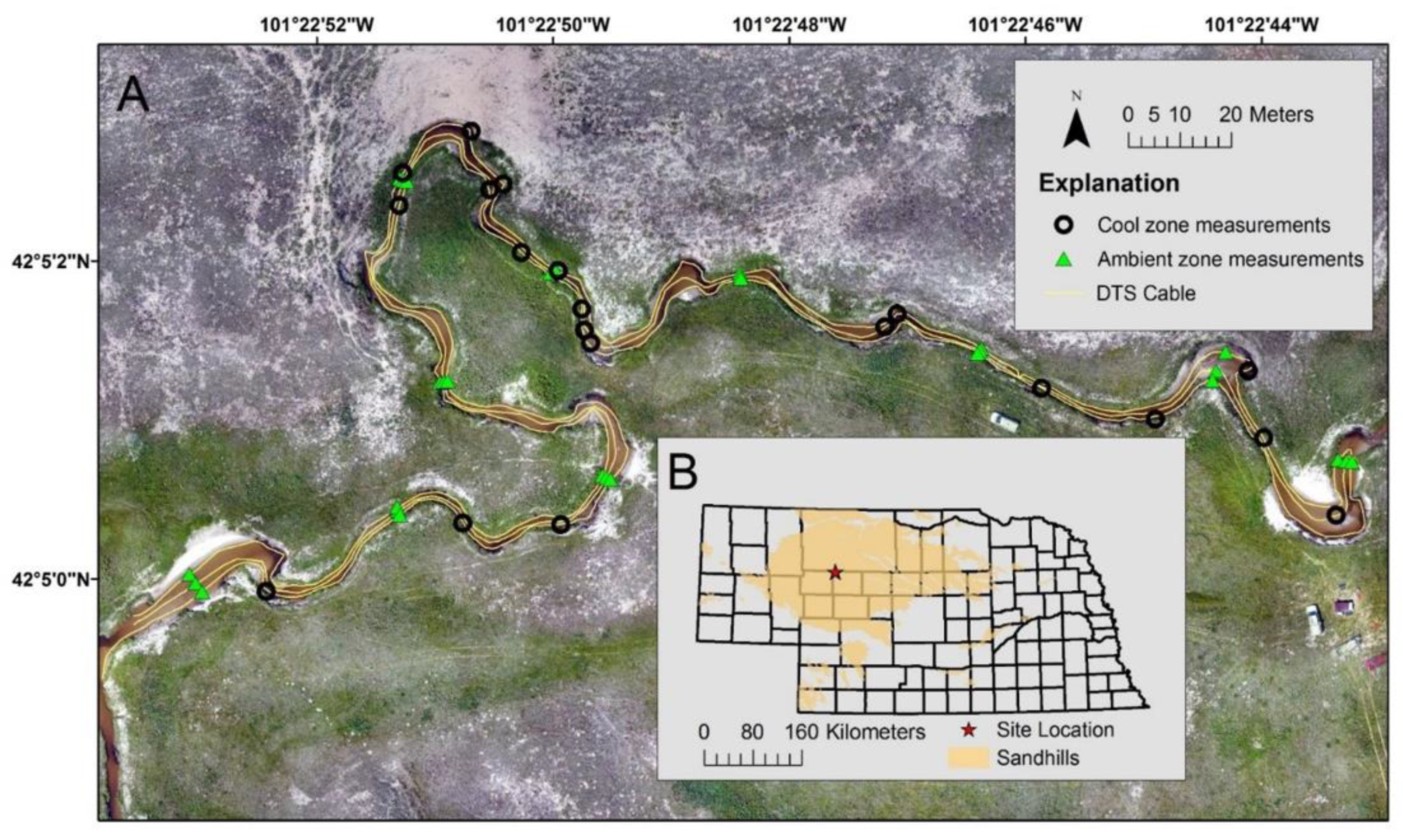
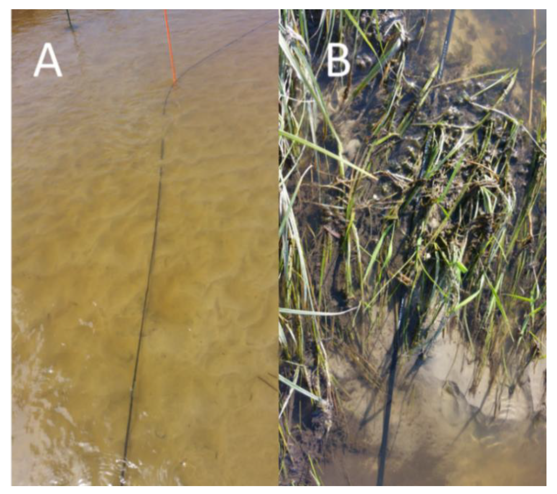
2.1. Site Description

The study was conducted on a 700-m reach on the South Branch of the Middle Loup River (SBMLR) on the University of Nebraska Gudmundsen Sandhills Research Laboratory land located in the central Sand Hills of Nebraska (Figure 1). The site is located in the northern region of the High Plains aquifer, where saturated thickness is 300 m. The SBMLR, a tributary to the Middle Loup and Loup Rivers, is a sinuous, second-order stream that drains approximately 925 km2 of pasture. The groundwater-fed stream has a stream width ranging from 2–5 m and water depth of 10–50 cm. Streamflow during the study period was about 250 L·s−1.
The sand dunes that comprise the Sand Hills are vegetated and minimally grazed. The soils and shallow subsurface aquifer near the study site are primarily eolian sand and loamy and sandy alluvium. The streambed consists of sand with some organic matter. Data from a previous study conducted upstream of our study site, where the organic matter content is much higher, suggested mean groundwater discharge rates of 0.1 to 0.3 m·day−1 through the streambed (based on estimated 2-m ditch width) [35,36]. These estimates are at the lower end of the range of other studies conducted using FO-DTS [4,26,37] (flux ranged 0.05 to 7.2 m·day−1) and similar to previous stream studies using physical measurement methods [2,18,21].

2.2. Identification of Uninformed and Informed Measurement Sites

Uninformed measurements were allocated at 16-m longitudinal intervals along the stream, for a total of 30 uninformed hydraulic measurements. The locations were predetermined without knowledge of streambed temperature dynamics. Beginning at the downstream end of the reach, intervals of 16-m longitudinal distance were measured, and a lateral three-point transect was marked across the stream (i.e., measurement locations at right bank, left bank, and center positions) at each interval.
To identify informed locations to measure streambed discharge, distributed temperature sensing with fiber-optic cables was used, and a total of 20 informed locations were identified. The FO-DTS unit was a Silixa-XT system provided by the Center for Transformative Environmental Monitoring Programs (CTEMPs). The FO-DTS control unit has a published linear spatial sampling resolution at 25 cm and an operating temperature from −40 to +65 °C at <0.01 °C resolution, although, in practice, the spatial resolution and temperature resolution are greater. FO-DTS theory applicable to our application can be found elsewhere [38,39,40].
The FO-DTS had 4000 m of Commscope flat-drop fiber-optic cable attached, although only 700 m of cable was deployed on the streambed at any given time during the study. The cable was attached to the control unit in double-ended mode, excess cable was left on a large spool, and temperature baths for DTS calibration were located between the spool and the stream. Temperature baths consisted of 10 m of cable placed in an ice bath in a cooler (0 to 3 °C) and an additional 10 m of cable placed in an ambient temperature water bath in a cooler. Each bath was equipped with a Silixa Pt100 temperature reference temperature probe, and an air bubbler circulator was used to avoid temperature stratification in the bath. Several air loops were also placed on the streambank or attached to stakes above the stream water level as spatial reference points.
The FO-DTS cable was secured on the streambed using clamps fastened onto vertical stakes (Figure 2). At the downstream end of the reach, approximately 100 m of stream length had FO-DTS cable deployed along the right bank, left bank, and center throughout the entire campaign. In the upstream part of the reach, the remaining 400 m of cable was sequentially placed on the right bank, then left bank, and then center of the stream during different time periods for groundwater discharge reconnaissance (starting 2 June 2017, 8 June 2017, and 9 June 2017, respectively). The movement of the cable to different streambed positions was done (1) to shorten the individual cable installation periods given the potential for precipitation events during the study period, and (2) to avoid temperature impacts of partial and/or temporary burial of large sections of the cable due to the mobile streambed. A third reason was that sequential installation also reduced the equipment (i.e., clamps and stakes) required for the detailed installation in the meandering channel.
After cable deployment along the right, left, or center of the stream, the streambed and cable were left undisturbed for a 12-h period. The unit logged temperatures along the length of the cable every 10 s at 25-cm sampling resolution during the campaign period. When data collection was complete for the right bank (4 June 2017; Figure 3), the end section of the cable (roughly 400 m) was moved to the left bank and left undisturbed for another 12-h period. This cycle was completed for center stream as well. The locations of the FO-DTS cable and the uninformed and informed measurement locations were identified using a survey-grade Topcon Hiper V global positioning system (GPS).
For each of these cable deployment locations (right bank, left bank, and center), uncalibrated temperatures (Figure 4C) were used for a field analysis of anomalies (i.e., cool zones, since the study was conducted in the summer). These anomalies were determined based on visual analysis of a temperature versus optical distance plot downloaded from the FO-DTS unit in the field (i.e., based on a “snapshot” of 10-s-averaged temperature measurements). For the deployment along the right side of the stream, the 10 most pronounced cool zones were identified for an equal comparison to the 10 uninformed measurements conducted along the right side. For the center and left side of the streambed, there were fewer pronounced cool zones and, therefore, fewer informed measurement locations.
After identification, the cooler sections of cable were located along the length of the physical cable based on cable length. Those cooler locations in the streambed were marked for informed measurements. The exact cable location where temperature anomalies existed were not known due to lack of precision in the cable sheathing. Even though the cable had numerical meter measurements, there were no tick marks on the sheath indicating where the meter marker started or ended, and there were also differences between the physical cable length and optical distance shown on the temperature plot. The long section of cable left on the spool may have also added some noise to the temperature data and contributed to this uncertainty. The general areas of cooler temperature zones were found first. A temperature probe (Fisherbrand™ Traceable™ Platinum Ultra-Accurate Digital Thermometer, seven-inch probe, ±0.05 °C accuracy) was then inserted into the streambed along the cable within these general areas. The point that had the lowest temperature based on the surrounding areas was identified as an informed location.
The DTS collected approximately 56,000 data points during the entire campaign. A subset of 2568 data points was post processed to represent the deployment period along the right bank and the 100 m of streambed where cable was left in the right bank, left bank, and center positions throughout the study for comparison to the field “snapshot” selection of informed sampling locations (e.g., Figure 3 and Figure 4). Post-processed data represented a 6-h period between 1:00 and 7:00 p.m. on 4 June 2017. The data for this period were calibrated using a MATLAB® graphical user interface (GUI) created by CTEMPs. The GUI allows the user to determine the location of the calibration baths and splice box in the collected data and use that information to calibrate temperatures collected by the DTS unit. This double-ended calibration method allowed for accurate calibration along two different channels within the same fiber-optic cable.

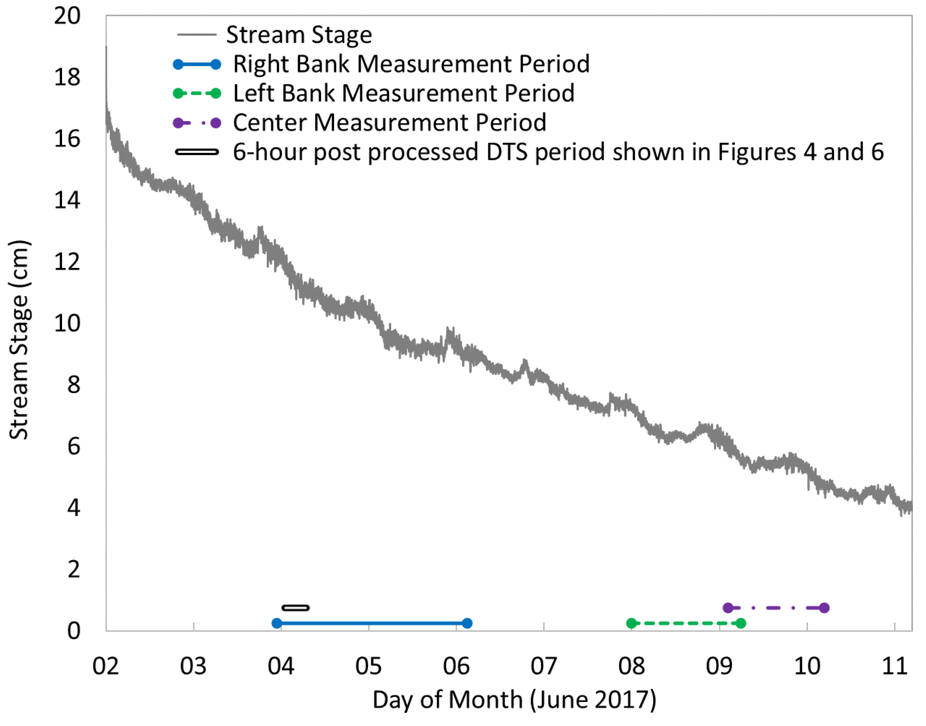
2.3. Hydraulic Measurements

Vertical hydraulic gradient (VHG; i, m∙m−1) and conductivity (Kv) were measured at each of the informed and uninformed locations. The VHG was measured between groundwater and surface water using a light-oil piezomanometer [9]. Firstly, VHG was measured to avoid the disruption of the local vertical hydraulic gradient. The hand-built piezomanometer was equipped with a drive-point screen (5 cm), which was pushed into the streambed to a depth of 30 cm (top of screen). Kv was estimated using the falling head permeameter method [41]. A permeameter, or clear polycarbonate tube with incremental markings on the side, was inserted into the streambed at 30 cm and a falling head test [41] was conducted. Kv was then calculated for each sampling location as described in previous work [41].
With i and Kv known, groundwater flux (q) was calculated for each of the 50 informed and uninformed locations as q = i × Kv.
A Sontek Flowtracker Acoustic Doppler Velocimeter was used for measuring stream discharge in the study reach and stream water velocity near the FO-DTS cable. Stream discharge measurements were made near the upstream and downstream ends of the study reach on 3 June 2017 and 5 June 2017 (n = 3). Stream velocity measurements were made at 45 locations with paired measurements made near the cable depth and higher in the water column (n = 90 stream velocity measurements).

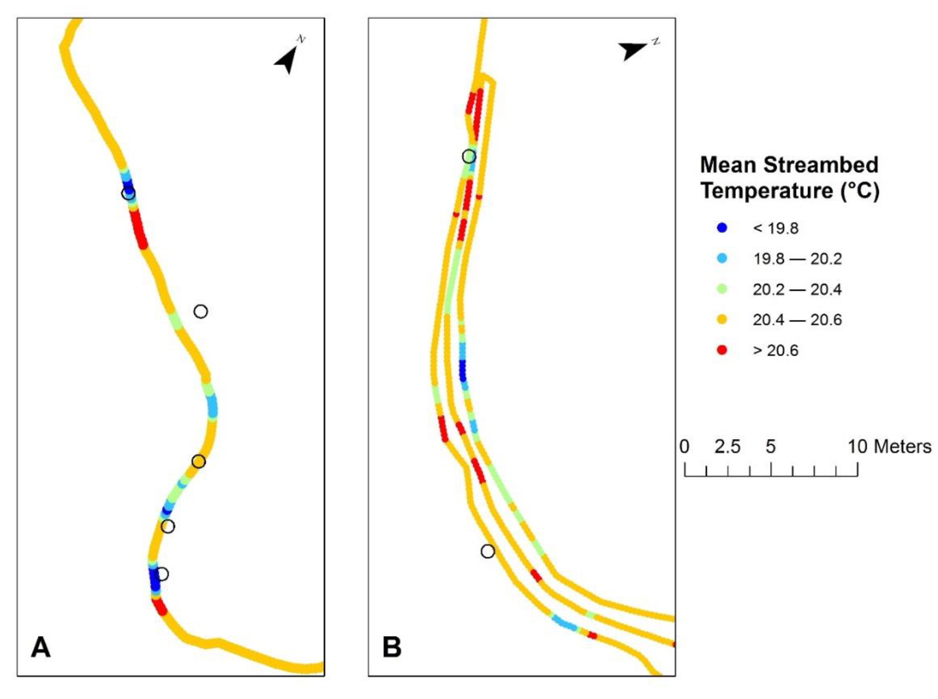
2.4. Drone Imagery Acquisition

During the course of FO-DTS temperature data collection, a DJI Phantom 4© Quadcopter with a 12-megapixel camera was used to collect aerial imagery of the study site. The resulting high-resolution orthophoto aided in digitizing the fiber-optic cable on the streambed (Figure 1) where there was uncertainty in GPS locations due to the remote study site location. The aircraft was pre-programmed to run a gridded flight pattern with roughly 70% image overlap for photogrammetric processing. Over 500 images were captured during the flight and then processed with the photogrammetric mapping software Pix4D©. Ground control points (GCP) with known GPS coordinates were previously placed in the streambed and at locations along the stream bank. These GCPs were imported into the mapping software, tagged to targets in the imagery, and used to create a georeferenced, seamless orthophoto of the site with ~1.4-cm spatial resolution.

3. Results and Discussion

FO-DTS and vertical flux measurement methods were combined in this study to address three research questions, each of which is discussed in the sections below. The fourth and final section is focused on the FO-DTS application and study limitations.

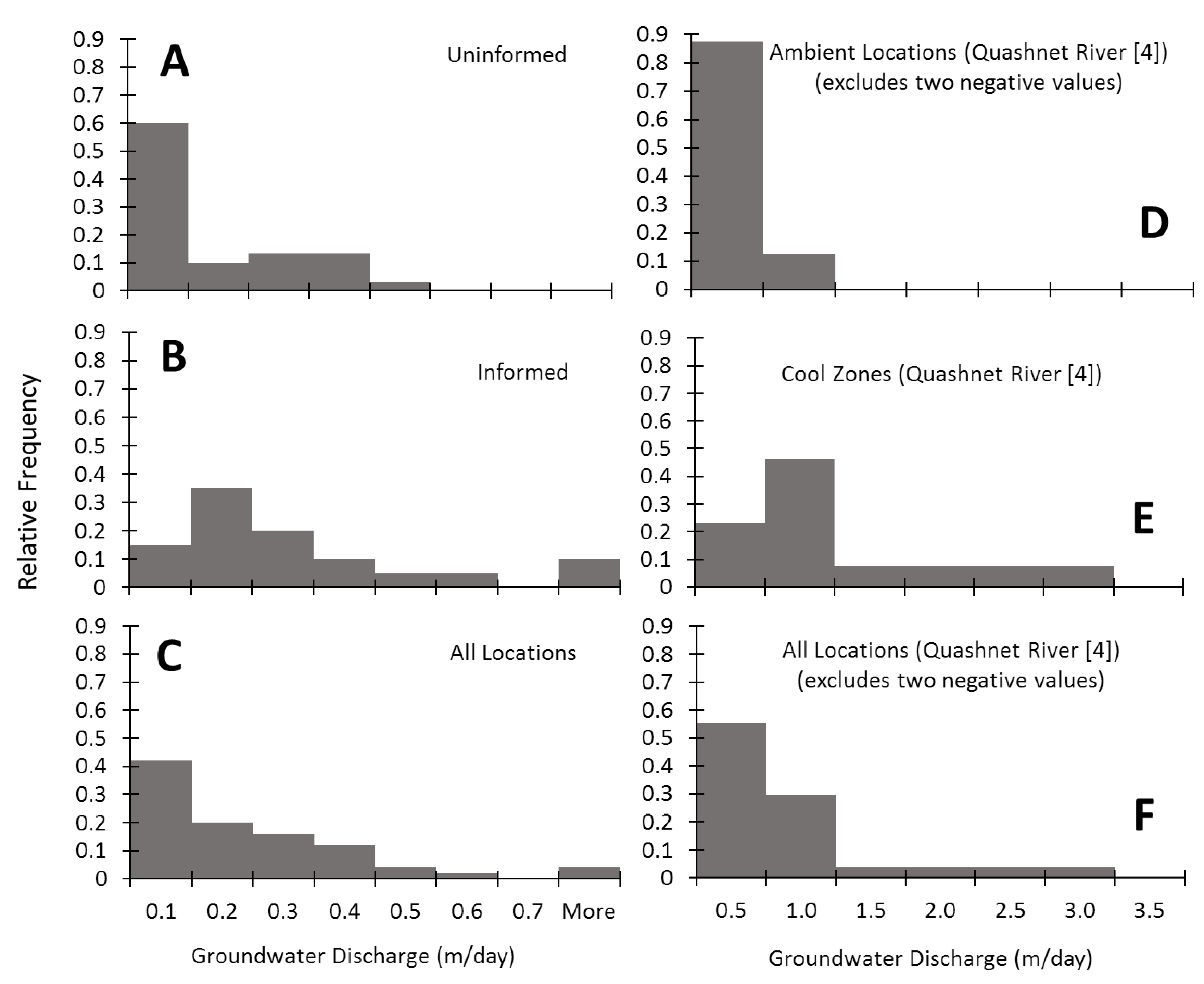
3.1. Are Discharge Estimates at Informed and Uninformed Locations Significantly Different?

All VHGs were positive, which indicated a consistent upward vertical groundwater flux during the study period. Median groundwater discharge for informed measurements was 0.21 m∙day−1, which was significantly higher than the median of uninformed measurements (0.05 m∙day−1) based on the Wilcox rank sum non-parametric U-test that is most appropriate for non-normal distributions (Table 1). Mean groundwater discharge for informed measurements (0.27 m∙day−1) was substantially higher than for uninformed measurements (0.12 m∙day−1).
Both vertical hydraulic conductivity (Kv) and head gradient (i) were on average lower for uninformed measurement locations than for informed locations, but the greatest difference was in Kv (Table 2). Median Kv for uninformed measurement locations was about 32% of Kv from informed locations and statistically different (U-test; α = 0.05, p = 0.024). The differences in Kv reflect how groundwater was preferentially discharging in areas with higher permeability. Uninformed i was about 82% of informed i. For informed measurement locations, variability (coefficient of variation) was greater for i than for Kv, and vice versa for uninformed measurement locations.

3.2. A Fundamentally Different View of Groundwater Discharge?

Although informed measurement locations yielded the highest groundwater discharge estimate (0.95 m·day−1), uninformed measurements had greater variability in discharge than informed measurements (coefficient of variation of 113% versus 91%, Table 1). In both cases, variability in groundwater discharge was in the range (on a percentage basis) of variability commonly observed in other streams, although the differences between informed and uninformed measurements were less pronounced in this study compared to differences in variability found previously [4] (174% versus 76% for ambient versus cool zones, Table 1).
The relative frequency distribution of all groundwater discharge measurements in the SBMLR (Figure 5C) is typical of other distributions observed in streams with sandy streambeds and relatively homogeneous connected aquifers [2,21,28]. In general, these distributions indicate a high frequency of measurements at low-discharge locations, with a long tail toward higher groundwater discharge values. The frequency distribution for uninformed measurements in our study reach was also heavily weighted toward low discharge values (Figure 5A). In comparison, the informed measurement locations yielded a broader distribution, including higher discharge values, but with the bulk of discharge in the moderate range (Figure 5B). Overall, the frequency distributions for informed and uninformed measurements represent fundamentally different distributions, based on the Kolmogorov–Smirnov test (D = 0.45, p = 0.012), as did the frequency distributions for ambient and cool zones measurements in the Quashnet River [4] (p << 0.01, exact p-value could not be computed due to “ties” in the two datasets). Thus, the use of FO-DTS in these systems led to substantially different views of groundwater discharge, based on statistically significant differences in both the median discharge and the frequency distributions for informed and uninformed measurements.
The shapes of the relative frequency for informed measurements in the SBMLR (Figure 5B) was remarkably similar to that of the cool zone measurements in the Quashnet River (Figure 5E) [4], albeit with almost a factor of five difference in magnitude of discharge. The frequency of low discharge values is clearly lower compared to ambient or uninformed measurements in either the Quashnet River or SBMLR. In contrast, the uninformed measurements had a broader distribution than the ambient locations selected in the Quashnet River, likely because our uninformed measurements sampled the streambed more broadly than the ambient location measurements purposely at relatively warm streambed zones for that study. In other words, it was possible for our uninformed measurements to occur at locations with high-, intermediate-, or low-temperature streambed zones, whereas ambient sites in the Quashnet River [4] were purposefully located in warmer streambed zones for comparison with measurements selectively located at cool zones.
The different observed frequency distributions are important to consider in future work, particularly for studies where the influence of groundwater chemistry on stream-water quality is a concern. There are potentially interesting tradeoffs between capturing groundwater chemistry at high-discharge points using FO-DTS, versus broader sampling that captures what appear to be high-frequency low-discharge points. For instance, studies of groundwater age and nitrate discharge from aquifers found highly variable groundwater age and nitrate concentrations in streambeds, and that high-versus low-discharge locations may be correlated with different nitrate fluxes [31,42]. Thus, it may seem intuitive to seek out and measure groundwater chemistry at high-discharge points using FO-DTS, but “missing” the high-frequency low-discharge points could potentially bias the overall estimates of chemical flux from groundwater and/or the distributions of groundwater age in aquifer discharge.
Furthermore, for studies where spatial interpolation is desired to upscale from streambed points to reach scale, it is important to capture both low and high discharge rates [20]. There may be opportunities in future work to exploit FO-DTS data in the field to better inform sampling strategy. For instance, streambed points may be selected at several temperature signatures (not just the warmest or coolest temperature anomalies) to capture the full spectrum of groundwater discharge rates. If temperature and groundwater discharge are reasonably correlated, FO-DTS may serve as a “line sample” along the streambed (e.g., Figure 6), and used to improve or evaluate spatial interpolation of streambed fluxes. On the other hand, a hybrid alternative is possible, where informed and uninformed sampling are combined to “randomly” sample the reach while also capturing potentially important high-discharge zones.

3.3. A Lower Discharge Threshold for Effective Use of FO-DTS?

Median groundwater discharge was 0.13 m·day−1 in this study, relatively low compared to the recent similar study [4]. In that study, they conservatively estimated a threshold of 0.42 m·day−1 as a cutoff below which FO-DTS application might be less effective for identifying focused discharge locations in the coastal Quashnet River. However, they noted that an argument could also be made for a smaller threshold of 0.2 m·day−1 and that, in other stream systems with lower stream velocities (less than the typical 0.5–1 m·s−1 observed in the Quashnet River), an even lower threshold could be applicable. Our study reach in the SBMLR had an average stream velocity along the FO-DTS cable of about 0.3 m·s−1. Thus, stream velocities and groundwater discharge rates at our site on the SBMLR are both lower than for the Quashnet River, suggesting the discharge rate threshold for successful application of FO-DTS for the geolocation of discharge points based on point-in-time temperature traces may indeed be <0.2 m·day−1, especially where stream velocities and other variables are favorable for the creation of discharge-based thermal anomalies.

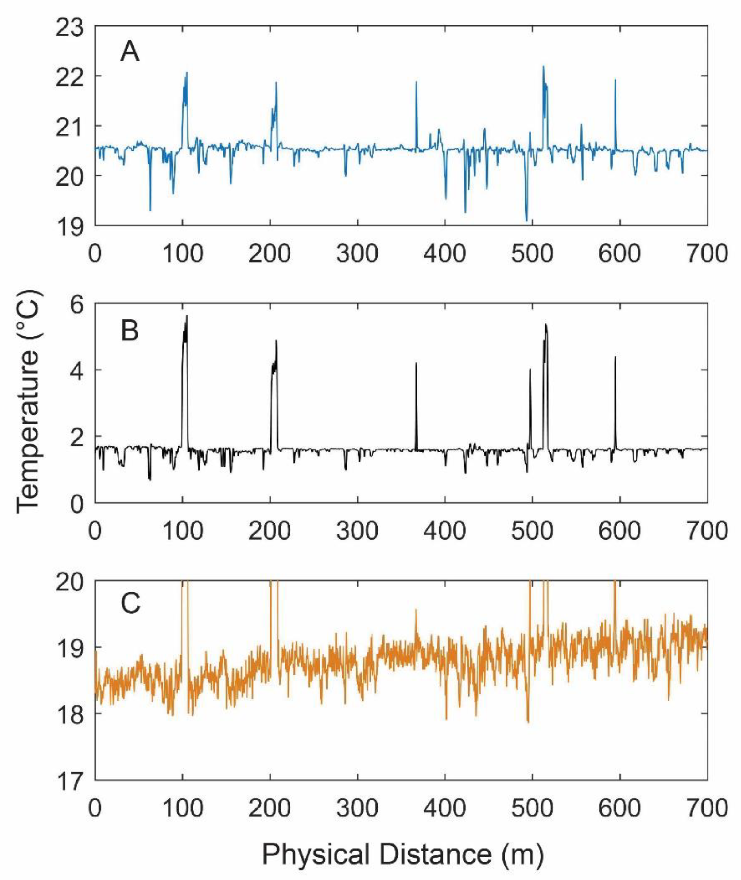
3.4. Raw vs. Calibrated FO-DTS Temperature Data and Study Limitations

One potential limitation to this study was the use of a less-precise “snapshot-in-time” approach to identify cool zones for informed measurement based on 10-s-averaged temperatures (Figure 4C; see also Section 2.2). A more robust in-field analysis of calibrated FO-DTS temperature data (Figure 4A,B), or even temperature averaged over a longer period (minutes, rather than seconds) may have led to more precise identification of cool zones. A subset of temperature data displayed in map view (Figure 6) suggests that the informed locations identified along the right bank in this study were reasonably consistent with post-processed and calibrated temperature data. Out of the seven measurement locations in Figure 6, five were located at or very near relatively cool locations as indicated by post-processed temperatures. The use of calibrated temperatures, mean streambed temperature, and temperature variance over time may eliminate some artefacts in the raw temperature data, and highlight areas that are consistently cooler, allowing for identification of subtle thermal anomalies corresponding to moderate flux zones. For example, parts of the cable in the direct sun could be affected more by solar radiation than parts of the cable that are in shaded areas. Integrating mean streambed temperature over a period of time may smooth out these direct solar warming-based variances [1].
However, more advanced approaches of post-processing FO-DTS temperature data in the field are time-consuming and could reduce the amount of physical measurements that can be made within a given study period. Lengthening the deployment measurement period increases potential for other artefacts as well. For instance, bedform migration in the stream channel can bury portions of the cable in the streambed, which would lead to a bias toward cooler streambed temperature, or possible misinterpretation of transience in groundwater discharge over time. Lengthened deployment and/or measurement periods also increase the risk of encountering significant transience in the system, including hydrological events that may create greater uncertainty in temperatures and even loss or damage of equipment (e.g., through deep burial of the cable, as we experienced at a larger river site). An approach that may help balance between lengthy post-processing and reserving sufficient time for physical measurements in the future is the use of temperature thresholds from FO-DTS temperature time series [4].
Due to topography, stream morphology, and the remote location of the research site, errors in GPS coordinates for measurement points and cable lengths mostly varied by roughly 0.10–1.0 m. Drone imagery was helpful for determining the cable location where GPS signal was poor. Other challenges included finding the exact locations of cool zones along the FO-DTS cable, as described previously in Section 2, and the time required to carefully deploy the cable along the right, left, and center of the meandering stream.

4. Conclusions

This field study quantitatively compared two different approaches for sampling streambed fluxes in space. The first approach used FO-DTS in a reconnaissance mode to identify likely zones of focused groundwater discharge in streambeds. We refer to this approach as informed measurement. These informed measurements were then compared to results from the more traditional approach of measuring streambed fluxes at evenly spaced transect locations selected without prior knowledge of streambed temperatures (uninformed measurements).
Streamflow in the Nebraska Sand Hills is dominated by groundwater discharge, which made our research site an ideal location for applying DTS methodology and for testing the hypothesis that informed groundwater discharge measurements would yield a significantly different view of groundwater discharge when compared with uninformed measurements. A non-parametric U-test showed a significant difference between median values for informed discharge measurements (0.17 m·day−1) and uninformed measurement locations (0.05 m·day−1). The frequency distributions for informed and uninformed measurements were also significantly different, based on a Kolmogorov–Smirnov test.
Areas of focused groundwater discharge were successfully identified in this study using a simple “snapshot-in-time” field analysis of FO-DTS data. Despite the less-precise raw data, results suggest a much lower threshold for the magnitude of groundwater discharge at which FO-DTS is applicable (approximately one-fifth of the value proposed previously [4]). Future studies that rely on more advanced post-processing of temperature data (to calibrate FO-DTS temperatures and remove artefacts in the data) may lead to even more precise identification of zones of focused groundwater discharge, although post-processing techniques need to be efficient enough to be conducted quickly in the field to guide sampling [43]. There has been a recent increase in the application of drone-based infrared thermal imaging for quick reconnaissance of groundwater discharge zones along streams at large scales [44]; however, infrared imaging does not penetrate the water column and low-to-moderate-discharge zones are likely to be missed.
Regardless of the approach to field analysis for FO-DTS, it is clear that temperature-based reconnaissance can lead to a substantially different view of groundwater discharge within a given stream reach. However, questions remain as to how application of FO-DTS may bias perceptions of overall average groundwater discharge into streams; it is important to carefully consider how FO-DTS fits into project objectives.

Author Contributions

Conceptualization, T.E.G. and M.A.B.; methodology, T.E.G., M.J. and J.K.; software, M.J.; validation, T.E.G., J.K. and A.M.; formal analysis, M.J., S.C. and T.E.G.; investigation, T.E.G., M.J., A.M., J.K., V.Z. and S.C.; resources, T.E.G., A.M. and J.K.; data curation, M.J., S.C. and T.E.G.; writing—original draft preparation, M.J.; writing—review and editing, T.E.G., A.M., J.K., V.Z. and M.A.B.; visualization, M.J. and T.E.G.; supervision, T.E.G.; project administration, T.E.G.; funding acquisition, T.E.G. and M.J.

Funding

This research was funded by the Daugherty Water for Food Global Institute, CTEMPS, and the US Department of Agriculture—National Institute of Food and Agriculture (Hatch project NEB-21-177). A portion of the analysis was funded by the USGS Toxic Substances Hydrology Program and by the National Science Foundation (EAR-1744719). The APC was funded by the Conservation and Survey Division—University of Nebraska.

Acknowledgments

The authors gratefully acknowledge Martin Wells for assistance with data collection. We are also grateful to Jacki Musgrave, John Nollette, and Andy Applegarth at the Gudmundsen Sandhills Research Laboratory for their insights and assistance in accessing the study site. Dave Gosselin also contributed to discussions about prior groundwater research at Gudmundsen. We gratefully acknowledge the CTEMPS support staff for their timely technical assistance during FO-DTS deployment and data processing. We also gratefully acknowledge three anonymous reviewers and one USGS reviewer who offered insightful suggestions that improved the manuscript.

Conflicts of Interest

The authors declare no conflicts of interest. The funders had no role in the design of the study; in the collection, analyses, or interpretation of data; in the writing of the manuscript, or in the decision to publish the results. Any use of trade, firm, or product names is for descriptive purposes only and does not imply endorsement by the US Government.

References

  1. Briggs, M.A.; Lautz, L.K.; McKenzie, J.M. A comparison of fibre-optic distributed temperature sensing to traditional methods of evaluating groundwater inflow to streams. Hydrol. Process. 2012, 26, 1277–1290. [Google Scholar] [CrossRef]
  2. Kennedy, C.D.; Genereux, D.P.; Corbett, D.R.; Mitasova, H. Spatial and temporal dynamics of coupled groundwater and nitrogen fluxes through a streambed in an agricultural watershed. Water Resour. Res. 2009, 45. [Google Scholar] [CrossRef]
  3. Krause, S.; Blume, T.; Cassidy, N.J. Investigating patterns and controls of groundwater up-welling in a lowland river by combining Fibre-optic Distributed Temperature Sensing with observations of vertical hydraulic gradients. Hydrol. Earth Syst. Sci. 2012, 16, 1775–1792. [Google Scholar] [CrossRef] [Green Version]
  4. Rosenberry, D.O.; Briggs, M.A.; Delin, G.; Hare, D.K. Combined use of thermal methods and seepage meters to efficiently locate, quantify, and monitor focused groundwater discharge to a sand-bed stream. Water Resour. Res. 2016, 52, 4486–4503. [Google Scholar] [CrossRef] [Green Version]
  5. Kalbus, E.; Reinstorf, F.; Schirmer, M. Measuring methods for groundwater—surface water interactions: A review. Hydrol. Earth Syst. Sci. Discuss. 2006, 10, 873–887. [Google Scholar] [CrossRef]
  6. Chen, X. Measurement of streambed hydraulic conductivity and its anisotropy. Environ. Geol. 2000, 39, 1317–1324. [Google Scholar] [CrossRef]
  7. Chen, X. Streambed Hydraulic Conductivity for Rivers in South-Central Nebraska1. Jawra J. Am. Water Resour. Assoc. 2004, 40, 561–573. [Google Scholar] [CrossRef]
  8. Chen, X.; Song, J.; Cheng, C.; Wang, D.; Lackey, S.O. A new method for mapping variability in vertical seepage flux in streambeds. Hydrogeol. J. 2009, 17, 519–525. [Google Scholar] [CrossRef]
  9. Kennedy, C.D.; Genereux, D.P.; Corbett, D.R.; Mitasova, H. Design of a light-oil piezomanometer for measurement of hydraulic head differences and collection of groundwater samples. Water Resour. Res. 2007, 43. [Google Scholar] [CrossRef]
  10. Briggs, M.A.; Lautz, L.K.; Buckley, S.F.; Lane, J.W. Practical limitations on the use of diurnal temperature signals to quantify groundwater upwelling. J. Hydrol. 2014, 519, 1739–1751. [Google Scholar] [CrossRef]
  11. Constantz, J. Heat as a tracer to determine streambed water exchanges. Water Resour. Res. 2008, 44. [Google Scholar] [CrossRef]
  12. Becker, M.W.; Georgian, T.; Ambrose, H.; Siniscalchi, J.; Fredrick, K. Estimating flow and flux of ground water discharge using water temperature and velocity. J. Hydrol. 2004, 296, 221–233. [Google Scholar] [CrossRef]
  13. Fanelli, R.M.; Lautz, L.K. Patterns of Water, Heat, and Solute Flux through Streambeds around Small Dams. Groundwater 2008, 46, 671–687. [Google Scholar] [CrossRef] [PubMed]
  14. Hatch, C.E.; Fisher, A.T.; Revenaugh, J.S.; Constantz, J.; Ruehl, C. Quantifying surface water–groundwater interactions using time series analysis of streambed thermal records: Method development. Water Resour. Res. 2006, 42. [Google Scholar] [CrossRef]
  15. Keery, J.; Binley, A.; Crook, N.; Smith, J.W.N. Temporal and spatial variability of groundwater–surface water fluxes: Development and application of an analytical method using temperature time series. J. Hydrol. 2007, 336, 1–16. [Google Scholar] [CrossRef]
  16. Schmidt, C.; Conant, B.; Bayer-Raich, M.; Schirmer, M. Evaluation and field-scale application of an analytical method to quantify groundwater discharge using mapped streambed temperatures. J. Hydrol. 2007, 347, 292–307. [Google Scholar] [CrossRef]
  17. Lowry, C.S.; Walker, J.F.; Hunt, R.J.; Anderson, M.P. Identifying spatial variability of groundwater discharge in a wetland stream using a distributed temperature sensor. Water Resour. Res. 2007, 43. [Google Scholar] [CrossRef]
  18. Solder, J.E.; Gilmore, T.E.; Genereux, D.P.; Solomon, D.K. A Tube Seepage Meter for In Situ Measurement of Seepage Rate and Groundwater Sampling. Groundwater 2016, 54, 588–595. [Google Scholar] [CrossRef]
  19. Kennedy, C.D.; Genereux, D.P.; Mitasova, H.; Corbett, D.R.; Leahy, S. Effect of sampling density and design on estimation of streambed attributes. J. Hydrol. 2008, 355, 164–180. [Google Scholar] [CrossRef]
  20. Conant, B. Delineating and Quantifying Ground Water Discharge Zones Using Streambed Temperatures. Groundwater 2004, 42, 243–257. [Google Scholar] [CrossRef]
  21. Gilmore, T.E.; Genereux, D.P.; Solomon, D.K.; Solder, J.E.; Kimball, B.A.; Mitasova, H.; Birgand, F. Quantifying the fate of agricultural nitrogen in an unconfined aquifer: Stream-based observations at three measurement scales. Water Resour. Res. 2016, 52, 1961–1983. [Google Scholar] [CrossRef] [Green Version]
  22. Matheswaran, K.; Blemmer, M.; Rosbjerg, D.; Boegh, E. Seasonal variations in groundwater upwelling zones in a Danish lowland stream analyzed using Distributed Temperature Sensing (DTS). Hydrol. Process. 2014, 28, 1422–1435. [Google Scholar] [CrossRef]
  23. González-Pinzón, R.; Ward, A.S.; Hatch, C.E.; Wlostowski, A.N.; Singha, K.; Gooseff, M.N.; Haggerty, R.; Harvey, J.W.; Cirpka, O.A.; Brock, J.T. A field comparison of multiple techniques to quantify groundwater–surface-water interactions. Freshw. Sci. 2015, 34, 139–160. [Google Scholar] [CrossRef]
  24. Sebok, E.; Duque, C.; Kazmierczak, J.; Engesgaard, P.; Nilsson, B.; Karan, S.; Frandsen, M. High-resolution distributed temperature sensing to detect seasonal groundwater discharge into Lake Væng, Denmark. Water Resour. Res. 2013, 49, 5355–5368. [Google Scholar] [CrossRef]
  25. Hare, D.K.; Briggs, M.A.; Rosenberry, D.O.; Boutt, D.F.; Lane, J.W. A comparison of thermal infrared to fiber-optic distributed temperature sensing for evaluation of groundwater discharge to surface water. J. Hydrol. 2015, 530, 153–166. [Google Scholar] [CrossRef] [Green Version]
  26. Poulsen, J.R.; Sebok, E.; Duque, C.; Tetzlaff, D.; Engesgaard, P.K. Detecting groundwater discharge dynamics from point-to-catchment scale in a lowland stream: Combining hydraulic and tracer methods. Hydrol. Earth Syst. Sci. 2015, 19, 1871–1886. [Google Scholar] [CrossRef]
  27. Briggs, M.A.; Harvey, J.W.; Hurley, S.T.; Rosenberry, D.O.; McCobb, T.; Werkema, D.; Lane, J.W., Jr. Hydrogeochemical controls on brook trout spawning habitats in a coastal stream. Hydrol. Earth Syst. Sci. 2018, 22, 6383–6398. [Google Scholar] [CrossRef] [Green Version]
  28. Browne, B.A.; Guldan, N.M. Understanding long-term baseflow water quality trends using a synoptic survey of the ground water-surface water interface, Central Wisconsin. J. Environ. Qual. 2005, 34, 825–835. [Google Scholar] [CrossRef]
  29. Puckett, L.J.; Zamora, C.; Essaid, H.; Wilson, J.T.; Johnson, H.M.; Brayton, M.J.; Vogel, J.R. Transport and fate of nitrate at the ground-water/surface-water interface. J. Environ. Qual. 2008, 37, 1034–1050. [Google Scholar] [CrossRef]
  30. Stelzer, R.; Drover, D.; Eggert, S.; Muldoon, M. Nitrate retention in a sand plains stream and the importance of groundwater discharge. Biogeochemistry 2011, 103, 91–107. [Google Scholar] [CrossRef]
  31. Kennedy, C.D.; Genereux, D.P.; Corbett, D.R.; Mitasova, H. Relationships among groundwater age, denitrification, and the coupled groundwater and nitrogen fluxes through a streambed. Water Resour. Res. 2009, 45, W09402. [Google Scholar] [CrossRef]
  32. Gilmore, T.E.; Genereux, D.P.; Solomon, D.K.; Solder, J.E. Groundwater transit time distribution and mean from streambed sampling in an agricultural coastal plain watershed, North Carolina, USA. Water Resour. Res. 2016, 52, 2025–2044. [Google Scholar] [CrossRef]
  33. Tesoriero, A.J.; Duff, J.H.; Saad, D.A.; Spahr, N.E.; Wolock, D.M. Vulnerability of streams to legacy nitrate sources. Environ. Sci. Technol. 2013, 47, 3623–3629. [Google Scholar] [CrossRef] [PubMed]
  34. Böhlke, J.K.; Denver, J.M. Combined use of groundwater dating, chemical and isotopic analyses to resolve the history and fate of nitrate contamination in two agricultural watersheds, atlantic coastal plain, Maryland. Water Resour. Res. 1995, 31, 2319. [Google Scholar] [CrossRef]
  35. Gosselin, D.C.; Drda, S.; Harvey, F.E.; Goeke, J. Hydrologic Setting of Two Interdunal Valleys in the Central Sand Hills of Nebraska. Groundwater 1999, 37, 924–933. [Google Scholar] [CrossRef]
  36. Gosselin, D.C.; (University of Nebraska, Lincoln, NE, USA). Personal communication, 4 October 2016.
  37. Vogt, T.; Schneider, P.; Hahn-Woernle, L.; Cirpka, O.A. Estimation of seepage rates in a losing stream by means of fiber-optic high-resolution vertical temperature profiling. J. Hydrol. 2010, 380, 154–164. [Google Scholar] [CrossRef]
  38. Selker, J.S.; Thévenaz, L.; Huwald, H.; Mallet, A.; Luxemburg, W.; van de Giesen, N.; Stejskal, M.; Zeman, J.; Westhoff, M.; Parlange, M.B. Distributed fiber-optic temperature sensing for hydrologic systems. Water Resour. Res. 2006, 42, W12202. [Google Scholar] [CrossRef]
  39. Selker, J.; van de Giesen, N.; Westhoff, M.; Luxemburg, W.; Parlange, M.B. Fiber optics opens window on stream dynamics. Geophys. Res. Lett. 2006, 33. [Google Scholar] [CrossRef] [Green Version]
  40. Tyler, S.W.; Selker, J.S.; Hausner, M.B.; Hatch, C.E.; Torgersen, T.; Thodal, C.E.; Schladow, S.G. Environmental temperature sensing using Raman spectra DTS fiber-optic methods. Water Resour. Res. 2009, 45, 11. [Google Scholar] [CrossRef]
  41. Genereux, D.P.; Leahy, S.; Mitasova, H.; Kennedy, C.D.; Corbett, D.R. Spatial and temporal variability of streambed hydraulic conductivity in West Bear Creek, North Carolina, USA. J. Hydrol. 2008, 358, 332–353. [Google Scholar] [CrossRef]
  42. Gilmore, T.E.; Genereux, D.P.; Solomon, D.K.; Farrell, K.M.; Mitasova, H. Quantifying an aquifer nitrate budget and future nitrate discharge using field data from streambeds and well nests. Water Resour. Res. 2016, 52, 9046–9065. [Google Scholar] [CrossRef]
  43. Domanksi, M.; Quinn, D.; Day-Lewis, F.; Briggs, M.A.; Werkema, D.; Lane, J. DTSGUI: A Python program to process and visualize fiber-optic distributed temperature sensing data. Groundwater. (under review).
  44. Harvey, M.C.; Hare, D.K.; Hackman, A.; Davenport, G.; Haynes, A.B.; Helton, A.; Lane, J.W.; Briggs, M.A. Evaluation of Stream and Wetland Restoration Using UAS-Based Thermal Infrared Mapping. Water 2019, 11, 1568. [Google Scholar] [CrossRef]
Figure 1. (A) Distributed temperature sensing (DTS) fiber-optic (FO) cable configuration on the streambed interface along ~700 m of stream channel. The cable was placed on the left bank, mid channel, and right bank at three distinct time periods throughout the study, as described in Section 2.2. Measurements were made at predetermined intervals, or “uninformed” locations along the fiber optic cable. Measurements were also made at “informed” locations of suspected high groundwater upwelling, which were indicated by cooler streambed temperatures sensed by the fiber optic cable. (B) Study site location in the central Sand Hills of Nebraska.
Water 11 02312 g001
Figure 2. (A) Fiber-optic cable deployed on the streambed, and (B) an example of areas where the cable was occasionally above the water line either due to difficulty in deploying the cable around bars in the channel, or due to a slight decrease in stream stage during the study period.
Water 11 02312 g002
Figure 3. Field campaign timeline in the month of June 2017. Sampling time periods for vertical head gradient measurements along the right bank, left bank, and center channel are indicated by horizontal bars. Uninformed sampling occurred toward the beginning of each sampling period, while informed sampling occurred toward the end of each sampling period. The horizontal black and white bar indicates the time period over which data collected by the DTS was post-processed (to correct for temperature offsets) and as an example of calibrated and time-averaged FO-DTS temperature data.
Water 11 02312 g003
Figure 4. (A) Post-processed DTS mean streambed temperature data over a 6-h time period on 4 June 2017. Peaks in the data represent air loops while troughs represent areas of cooler temperature zones. (B) Standard deviation of temperature data for the same period. Large peaks in the data indicate high variability in air temperature at air loops. (C) Single snapshot of one temperature signal captured by the DTS on 4 June 2017. This raw (uncalibrated) dataset was used for selecting where informed physical measurements would be taken. Note that the full scale of temperature at air loops is not shown in (C).
Water 11 02312 g004
Figure 5. Relative frequency distributions of (A) informed, (B) uninformed, and (C) all groundwater discharge measurements in this study, alongside frequency distributions calculated from (D) ambient locations and (E) cool locations, and (F) calculated from all groundwater discharge measurement locations reported from the Quashnet River in a separate study [4]. Two negative (downward) flux estimates were excluded from the ambient and all measurement distributions from the Quashnet River. Labels on the horizontal axis indicate the upper limit for each bin.
Water 11 02312 g005
Figure 6. Calibrated mean streambed temperature for the time period shown in Figure 3. Informed sampling locations (shown as open circles) are along the right bank of the stream (A) in the upstream part of the reach where a single strand of cable was placed, and (B) in the downstream end of the reach where cable was left in the right bank, left bank, and center positions throughout the campaign.
Water 11 02312 g006
Table 1. Summary statistics for groundwater discharge (q) measurements in this study and in a previous study [4].
This StudyQuashnet River [4]
AllUninformed aInformed aAllAmbient aCool a
Median (m·day−1)0.130.05 b0.21 b0.400.170.83
Mean (m·day−1)0.180.120.270.580.191.07
Standard Deviation (m·day−1)0.200.140.250.740.330.81
Coeffiecient of Variation (%)1101139112617476
Min (m·day−1)<0.01<0.01<0.01−0.55−0.550.20
Max (m·day−1)0.950.480.953.00.933.0
Measurements (-)503020291613
a A subtle difference in nomenclature, as described in the introduction: in previous work [4], groundwater discharge was measured at 29 locations, all selected based on fiber-optic distributed temperature sensing (FO-DTS) data, and classified results as ambient or cool zone measurements. In this study, we pre-selected measurement locations without any prior knowledge of streambed temperature (uninformed) and compare those discharge values with those measured at cool zones (informed). b Statistically different values (α = 0.05, p = 0.027).
Table 2. Summary statistics for head gradient (i) and vertical hydraulic conductivity (Kv).
AllUninformedInformed
i (m·m−1)Kv (m·day−1)i (m∙m−1)Kv (m·day−1)i (m·m−1)Kv (m·day−1)
Median0.0186.80.0173.5 a0.02311.1 a
Mean0.0238.60.0206.00.02812.4
Standard Deviation0.0238.50.0136.30.03210.0
Coefficient of Variation99%99%65%105%115%80%
a Statistically different values (α = 0.05, p = 0.024).

