Multi-Method Tracking of Monsoon Floods Using Sentinel-1 Imagery
by
 , and
, and
Giuseppe Ruzza
1,*, 
Luigi Guerriero
1,
Gerardo Grelle
2,
Francesco Maria Guadagno
1 and
Paola Revellino
1 1
Department of Science and Technology, University of Sannio, 82100 Benevento, Italy
2
Department of Civil, Building and Environmental Engineering (DICEA), Sapienza University of Rome, 00184 Rome, Italy
*
Author to whom correspondence should be addressed.
Water 2019, 11(11), 2289; https://doi.org/10.3390/w11112289
Submission received: 24 September 2019
/
Revised: 28 October 2019
/
Accepted: 29 October 2019
/
Published: 31 October 2019
(This article belongs to the Special Issue Improving Flood Detection and Monitoring through Remote Sensing)
Abstract
:Floods cause great losses in terms of human life and damages to settlements. Since the exposure is a proxy of the risk, it is essential to track flood evolution. The increasing availability of Synthetic Aperture Radar (SAR) imagery extends flood tracking capabilities because of its all-water and day/night acquisition. In this paper, in order to contribute to a better evaluation of the potential of Sentinel-1 SAR imagery to track floods, we analyzed a multi-pulse flood caused by a typhoon in the Camarines Sur Province of Philippines between the end of 2018 and the beginning of 2019. Multiple simple classification methods were used to track the spatial and temporal evolution of the flooded area. Our analysis indicates that Valley Emphasis based manual threshold identification, Otsu methodology, and K-Means Clustering have the potential to be used for tracking large and long-lasting floods, providing similar results. Because of its simplicity, the K-Means Clustering algorithm has the potential to be used in fully automated operational flood monitoring, also because of its good performance in terms of computation time.
1. Introduction
Floods are among the most frequent and widespread natural hazards in the world. Being related to intense and/or extreme weather events, they cause great losses in terms of human life and damage to commercial and productive sites, infrastructures, and agriculture [1,2]. Particularly, it has been estimated that floods are responsible for approximately 40% of the total damage caused by natural hazards [3,4]. Exposure to flooding is considered a proxy of the risk [5], so that an evaluation of the extent of potentially inundated areas is crucial for hazard and risk assessment and represents the basis for land planning and policy decisions oriented towards flood mitigation (i.e., occupation restrictions, recommended uses, and flood insurance plan development). Flood hazard and risk evaluations can be completed using the results of deterministic hydrodynamic models that simulate water movement across the floodplain. In the presence of monitoring (fluvial stage or discharge) and topographic data, statistical models associated with GIS processing can provide a basis for such kinds of analyses [6,7,8]. Both deterministic and statistical models need to be calibrated and validated using available flood data in terms of spatial extent, persistence, and frequency.
Data derived from a number of satellite platforms can be used to image floods, providing a basis for a rapid and effective response to natural disasters. Satellite observations have the advantage of covering large areas with an increasingly short revisiting time, which makes them able to support continuous observation and operation monitoring of floods [9,10]. Among different satellite data, Synthetic Aperture Radar (SAR) products provide an opportunity to image floods because of their all-weather and day/night capability [11,12] and their sufficient resolution for urban and suburban mapping [13,14]. SAR observation capabilities through clouds allow tracking flood events connected to prolonged rainfall [15]. SAR data have been widely used to study this kind of event in different contexts and have the potential to support surface water operational monitoring [16]. Giustarini et al. [17] and Mason et al. [18] used SAR data for flood detection in an urban area. They provided a way to image floods also in contexts where it is difficult to separate water by land. For instance, Martinis et al. [19] used Sentinel-1 data to improve flood monitoring in arid areas, where the similarity between radar backscattering of open water and sand surfaces led to an overestimation of the water extent. SAR data allow floods to be imaged over very large areas. In this context, Xing et al. [20] monitored monthly changes in surface water of Dongting Lake. Space-born L-Band SAR data were used by Chapman et al. [21] to map regional inundation events on the continental scale. Water flood information produced by SAR imagery can be also associated with additional remote sensing data (e.g., multispectral and optical imagery) for detecting the flooding extent and evolution in what we could define as a multi-data/methods approach. For instance, Refice et al. [22] used multi-sensor and multi-temporal remote sensing approaches to characterize flooding that affected part of the Strymonas river basin, a transboundary river with its source in Bulgaria, which flows then through Greece up to the Aegean Sea. Hakdaoui et al. [23] used radar and optical data to extract geomorphological information after a flash flood event in a Saharan arid region, and Shuman et al. [24] used SAR data and aerial photography to track urban flood dynamics.
Many methodologies have been proposed in the literature for the identification of flooding from SAR images. Texture recognition algorithms [25], histogram thresholds [26], and various multi-temporal change detection methods [17] are examples of these methodologies. Bioresita et al. [27] constructed an automatic chain process for surface water extraction. An unsupervised method, based on stochastic subspace ensemble-learning, was proposed by the authors of [28]. Schlaffer et al. [29] used a harmonic analysis and change detection to extract flooded areas, and an unsupervised approach, based on a generalized Gaussian model, to automatically detect surface change was used by the authors of [30]. Many authors (e.g., [31,32,33]) proposed and used an automated method for the extraction of surface water from SAR data based on supervised and unsupervised approaches. Additional authors like Bayik et al. [34] used multiple classification methods to improve flood mapping from SAR images. Since such methods have a variable degree of complexity (i.e., required parameters in relation to algorithm complexity) and attitudes from an automatic operational monitoring perspective, a number of comparisons have been proposed in order to underline the advantages and disadvantages of each method (e.g., [35]).
On this basis, and in order to further contribute to a better evaluation of the potential of SAR imagery in tracking large and long-lasting multi-pulse floods, we comparatively analyzed simple classification methods that might be suitable for automatic flood monitoring. Notably, the aim of this paper was to demonstrate the suitability of SAR products to image floods and quantify the magnitude of variation in the flooding extent derived by the use of multiple classification methods for the same event. In this perspective, we used Sentinel-1 imagery to track the evolution of a flood event that occurred in the monsoon area of the Philippines. The event, caused by torrential rains, occurred at the end of December 2018, persisted until the end of February 2019, and affected approximately 680,000 people. The area of Camarines Sur Province, in the eastern Philippines, suffered the most substantial effects. This event represents a very important case in history because of its effects, the extent of the involved area, and its duration, which makes it suitable for a SAR-based analysis and comparison between multiple classification methods.
2. Study Area
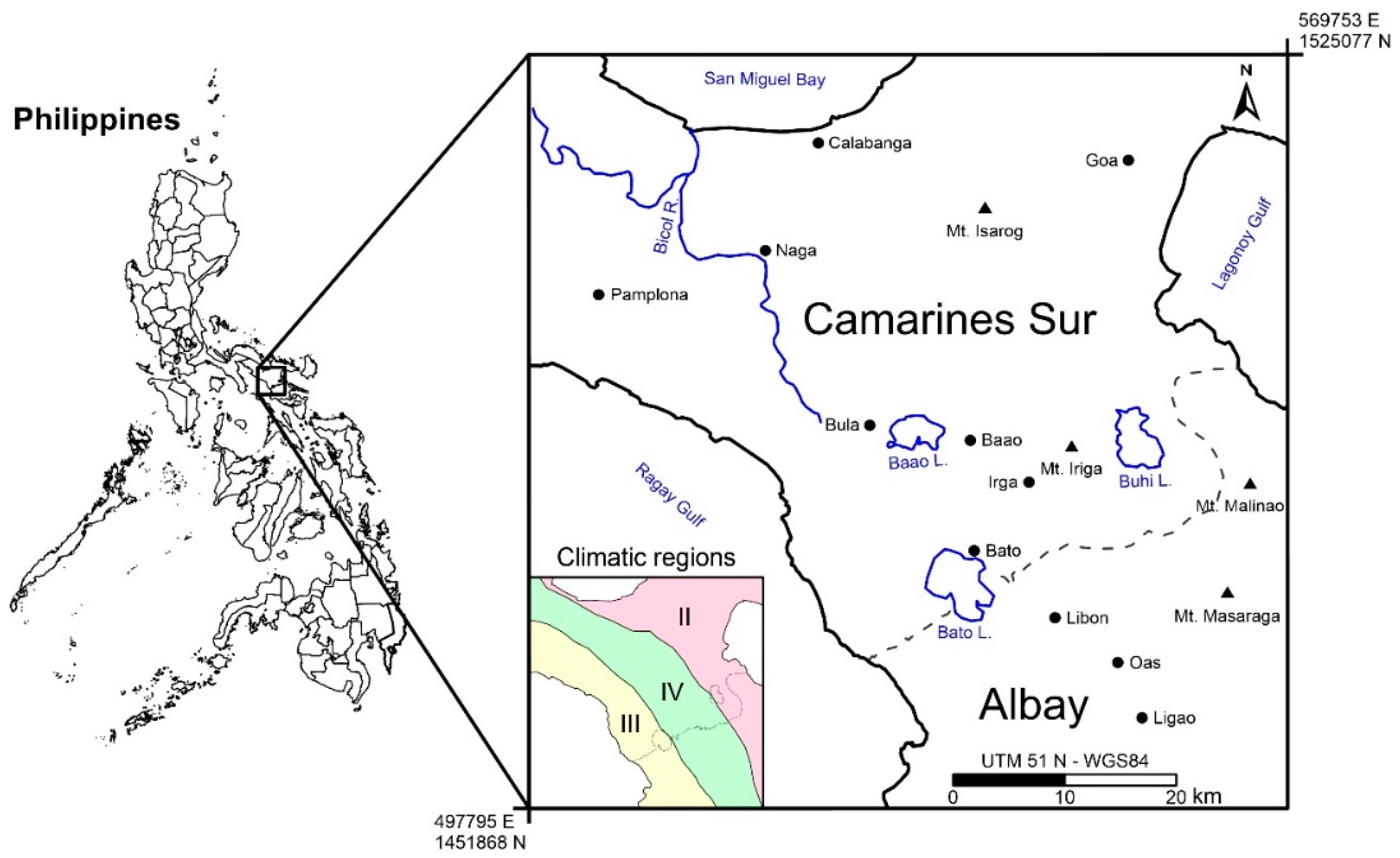
This study area included the Camarines Sur Province and a small portion of the Albay Province (Figure 1) located in the Bicol Region in Luzon of the Philippines. The Camarines Sur Province occupies the central section of the Bicol Peninsula and is the largest province in the Bicol Region. The Bicol River is the main watercourse of the province and is surrounded by Mount Isarog (1966 m asl) and Mount Iriga (1196 m asl). The eastern portion of the province lies on the mountainous peninsula of Caramoan, which faces the island of Catanduanes to the east. The Bicol River drains the central and southern parts of the province toward the San Miguel Bay. Mount Iriga is surrounded by three lakes named Buhi, Bato, and Baao. The Albay Province is generally mountainous with scattered valleys. On the eastern part of the province is a line of volcanic mountains starting with the northernmost Malinao in Tiwi and followed by Mount Masaraga (1328 m asl) and the Mayon Volcano (2463 m asl).
The Philippines archipelago has a tropical and strongly monsoonal climate characterized by relatively high temperature, oppressive humidity, and plenty of rainfall. Two main seasons alternate for the majority of islands, a wet season dominated by monsoon rainfall and a dry season. Some areas experience rainfall throughout the year, and clear season alternations are absent. Four climate regions are recognizable across the Philippines archipelago characterized by different distributions of rainfall [36,37]. The study area spans across three of these four climatic regions (Figure 1): region II is characterized by the absence of a dry season with a very pronounced maximum rainfall during the months of November and December, region III is characterized by a slightly drier seasons between November and April and a wet season between May and October, and region IV is characterized by rainfall distributed throughout the entire year. From June to December, tropical cyclones (typhoons) often strike the Philippines. Most of these storms come from the southeast and are heaviest in Samar, Leyte, south-central Luzon, and the Batan Islands, and, when accompanied by floods or high winds, they may cause great loss of life and properties.
In December 2018, as reported by the Department of Science and Technology (PAGASA) of the Republic of Philippines (http://bagong.pagasa.dost.gov.ph/tropical-cyclone), the study area was flooded as a consequence of a typhoon induced by a tropical depression (named “Usman”). This was the 21st and the last cyclone that intersected the Philippines in 2018. The “Usman” depression, developed from tropical disturbances, resulted in widespread heavy rainfall over large portions of Southern Luzon and Eastern Visayas. From 28 to 29 December 2018, prolonged and excessive rainfall over these areas resulted in multiple landslides and floods. Of the 139 stations with reliable data, the highest 2-day rainfall was estimated at 573.2 mm and was recorded in Daet (Camarines Norte), 50 km away from the study area. In the week preceding the event, rainfall accumulations in excess of 100 mm were already observed by multiple rain gauges over the eastern section of Luzon and Visayas, especially over Bicol Region mainland, Samar island, Aurora, Quezon, and Rizal. The event caused hundreds of casualties and millions of dollars in damages to personal and public property. According to the report of the Department of Social Welfare and Development (DSWD), more than 680,000 people were affected by the storm. Nearly 55% were located primarily in the province of Camarines Sur in the Bicol Region. Over 1900 homes were destroyed, and more than 15,000 were damaged. Agricultural losses were estimated at PHP 2 billion (US $37 million), with over 56,000 farmers and fishers affected, according to the United Nations Food and Agriculture Organization.
3. Data and Methods
3.1. Data
To quantify the extent of the flooded area, i.e., the area covered by open water, and track its spatial and temporal evolution, we used multiple Sentinel-1 A/B SAR images. The satellite data were downloaded from the Copernicus Open Data Access Hub (https://scihub.copernicus.eu/dhus/#/home). Sentinel-1 data products consist of imagery with a medium resolution (10–20 m) that represents the radar echo from the surface of the Earth of the signal emitted by the onboard antenna of the satellite. The Sentinel-1 satellite constellation is formed by two satellites (S-1 A and S-1 B) characterized by an acquisition frequency of six days. Each satellite is equipped with a 5.405 GHz C-band (λ ≈ 5.6 cm) imager payload (CSAR). The CSAR instrument supports operation in dual-polarization (HH + HV and VV + VH). The Sentinel-1 satellites can operate in three imaging modes for various observation approaches, spatial resolutions, and swath widths [38]. In this study, we used a total of 24 images with VV polarization. We chose this polarization because it characterized all of the selected data; only a limited number of images were acquired in double polarization VV + HH. VV polarization, in some cases, provides better results in detecting open water features [39,40]. The selected images had the same angle of incidence (38.8°) and footprint and were acquired in descending mode. The selected images covered the time period between 13 November 2018, prior to the typhoon, and 18 March 2019, after the typhoon. The first selected image was acquired 78 days before the main flooding event, occurring between 28 and 29 December 2018. This long pre-event time span allowed us to observe the normal fluctuations of the open water area before the flood.
3.2. Data Pre-Processing
Waterbody identification and extraction were completed considering the difference in the backscattering coefficient (Gamma γ°) between open water and the land surface. This difference is related to the roughness of the target surface, which is regulated by the Rayleigh criterion. Since the open water theoretically has no roughness, the incident radiation is reflected away from the sensor; thus, the backscattering coefficient related to its flat surface is lower than the land surface [41,42,43]. In contrast, the land surface that has a variable roughness has a variable backscattering coefficient typically higher than that characterizing open water. SAR imagery, downloaded by Sentinel Data Hub, were pre-processed using the Sentinel Application Platform (SNAP) toolkit distributed by ESA (https://step.esa.int/main/toolboxes/snap/). The products were first cropped across the area of interest to allow for shorter processing times. Subsequently, radiometric calibration was applied, and terrain was corrected to the Gamma band (i.e., backscatter coefficient γ°) [44]. To complete this last step, the STRM 1 arc-second digital elevation model (DEM) was used. Finally, in order to obtain high-quality SAR images and reduce the noise, we applied the Lee-Sigma filter [45,46] characterized by a combination of 5 × 5 and 7 × 7 windows.
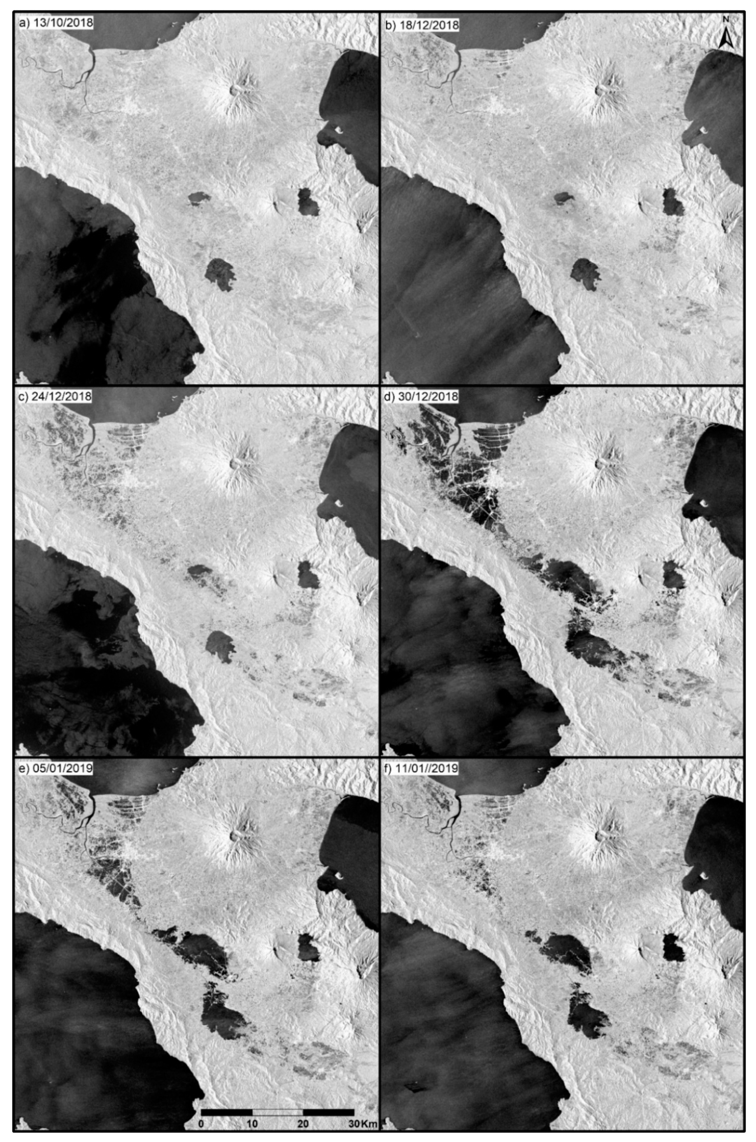
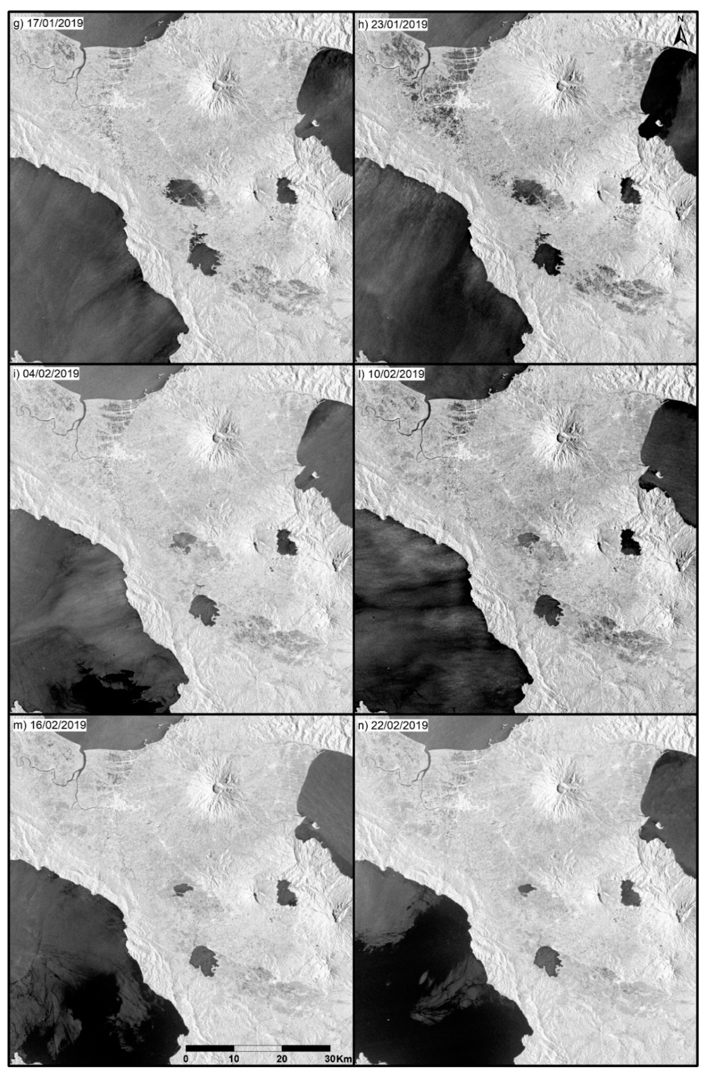
As the last step of image pre-processing, calibrated and filtered SAR images were cropped over the land of the study area. This was done in order to remove (from images and relative histograms) the changing backscattering effects induced at the ocean surface by the difference in wind conditions that generating waves mimicked the surface roughness, which produced a double-bounce effect [47]. After pre-processing, the rearranged backscatter intensities were converted into dB (decibels). Figure 2 and Figure 3 show a selection of 12 SAR images, out of 24 used, in which it is possible to visually identify the different flood traces of the events.
3.3. Extraction of the Water Body Area
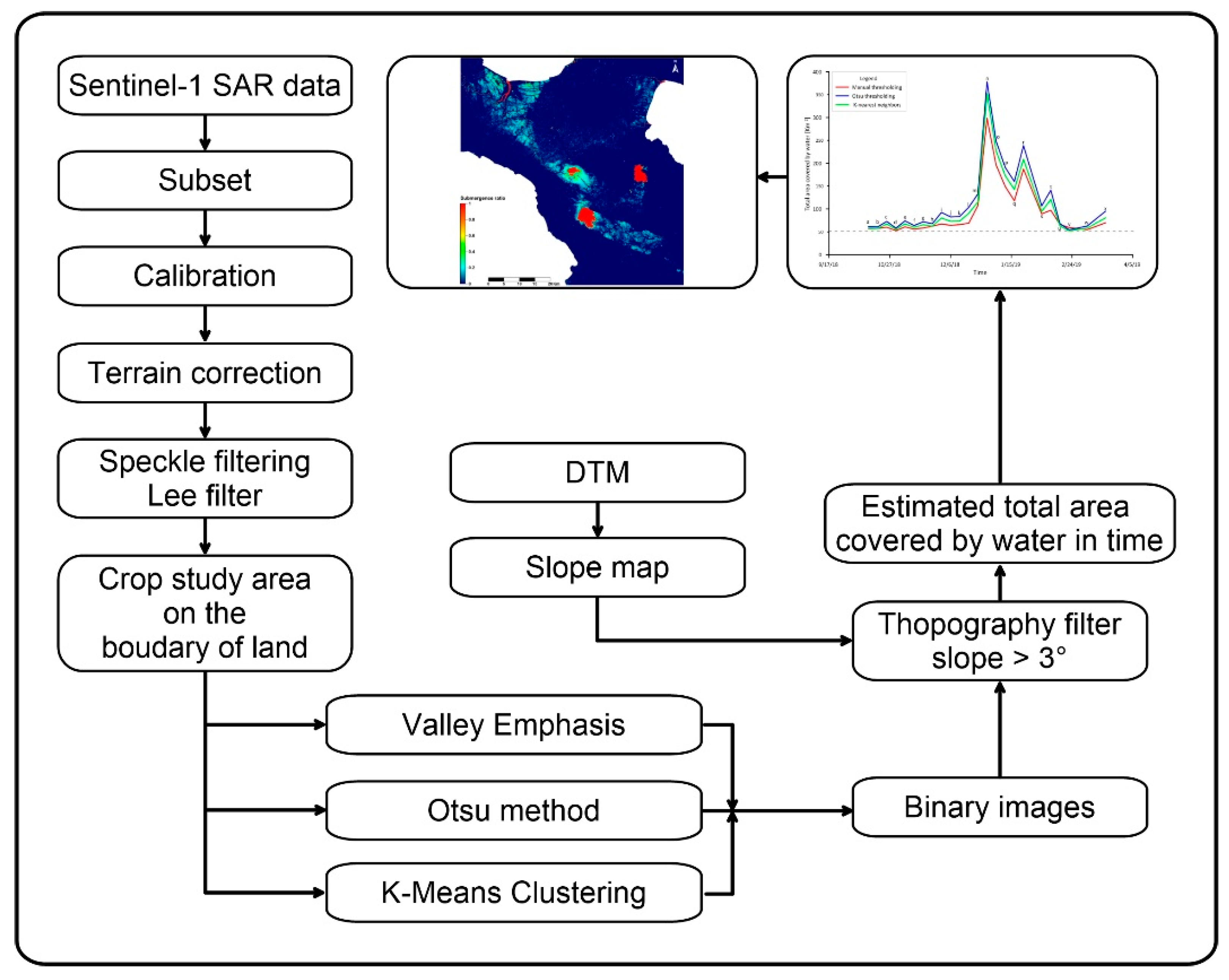
Figure 4 summarizes the workflow used to process images and quantify the total water area in the reference time period. In order to identify the open water features to determine the total area covered by water and its spatial and temporal evolution due to monsoon flood events, three different classification methods were applied that might have the potential to be used in operational monitoring. Our multi-method approach allowed us to compare specific results and quantify relative differences (e.g., [48,49]) in order to identify the best method to be used from an operational monitoring perspective. Particularly, we used two methods based on threshold identification and a third based on unsupervised K-Means Cluster analysis. Threshold-based methods are widely used because of their efficiency in identifying flooded areas in SAR images [50,51,52,53]. These methods consisted of defining a fixed value for the backscattering coefficient (i.e., intensity) that split the histogram in two subsets (clusters), one subset representing the land surface and the other representing the open water. Pixels with a low grayscale intensity typically corresponded to water bodies, while pixels with high values corresponded to the land (in our case, background). There are several techniques (supervised and unsupervised) to find the optimal threshold value [54,55,56,57]. Among these, for our comparative analysis, we selected visual identification of the threshold guided by the Valley Emphasis criterion, the Otsu method, and the unsupervised classification method based on K-Means Clustering.
The first method consisted of visually inspecting a grayscale histogram of each SAR image and applying the Valley Emphasis criterion [58,59,60]. For the application of this criterion, we first analyzed the grayscale histogram in SNAP and, subsequently, chose the minimum backscatter intensity value that corresponded to the valley between the two peaks, in the case of bimodal distribution, or to the bottom rim of a single peak for a unimodal distribution. Once identified, we converted this intensity value from dB to a “grayscale” value between 0 to 255 (8-bit images). The identified threshold value was then used as a basis for manual image classification. Image classification was consistently completed in the GIS environment (QGIS 3.7), assigning 0 to pixels with values higher than the threshold (i.e., land) and 1 to pixels with values lower than the threshold (i.e., water). After classifying the images, and considering that low backscattering intensity values can be also related to the presence of shadow zones (i.e., not only to the presence of water), especially in presence of complex topography, we used a further classification method based on topographic attributes to identify and exclude these areas from our analysis. Notably, we generated a slope map using the available STRM 1 arc-second DEM and used a slope threshold of 3° to exclude the low backscattering areas with slopes higher than the threshold.
The second method used to find the correct threshold value was the Otsu method. This method is widely used in applications where it is necessary to split grayscale images into two different classes. This method automatically chooses the threshold value from the grayscale histogram on the basis of the minimum within-class variance or the maximum between-class variance [61]. The Otsu method is commonly used because of its simplicity, and the best results are obtained if the image histogram is characterized by a bimodal or multimodal distribution. In the presence of a unimodal distribution, this method fails. The Otsu method for finding an optimal threshold value for image classification was applied in the Matlab™ environment. The Otsu threshold was then used to classify the images with the same procedure used as the previous method.
The last method was the K-Means Cluster analysis. This clustering method is a statistical technique widely used for dimensional reduction and has the potential to be used for unsupervised analysis of SAR images [62,63]. In our case, K-Means Clustering was used for dividing the image in two classes (i.e., water and land clusters). This method groups pixels on the basis of their grayscale level distribution and standard deviation. The purpose of this algorithm is to reduce variability within clusters, and the objective function is the sum of square distances between cluster centers and its assigned pixel value [64]. This clustering method, implemented in the SNAP toolbox, was applied considering two clusters, 30 interactions, and 32,000 random seeds. After cluster identification, the topographic filter and subsequent manual classification of the images were completed. Finally, we estimated the total water area in each image.
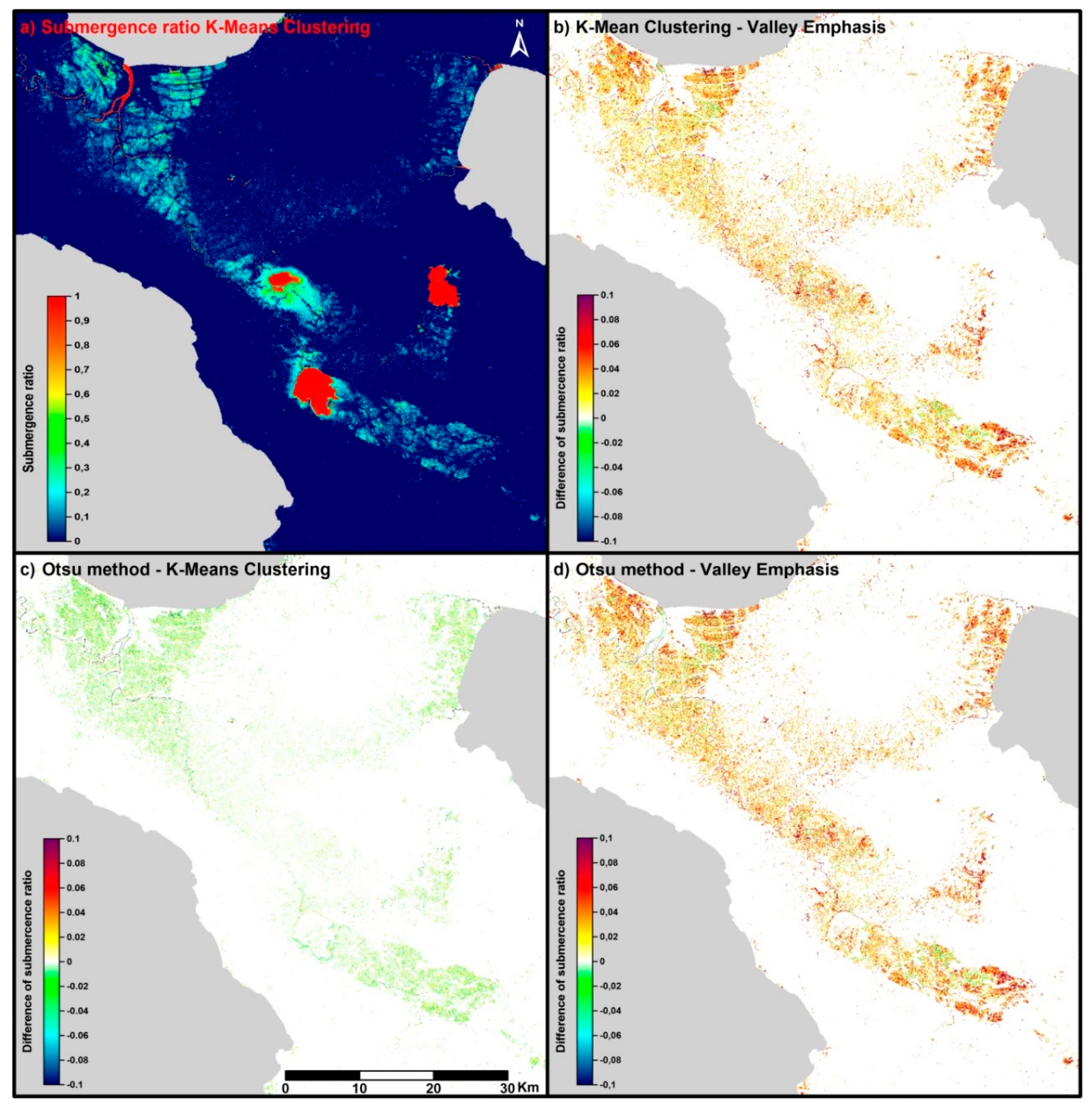
Once the spatial extent of open water features across the study area was evaluated, to further analyze the spatial and temporal distribution of flood intensity and persistence, and its change between the different methods, we estimated the submergence ratio across the whole of the study area and the reference period, and we compared this ratio in terms of arithmetic differences between products derived by our data (i.e., water area extent) obtained by different methods. A submergence ratio equal to 1 indicated the constant presence of water in the reference area, while a value of 0 indicated the constant absence of water in the reference area and across the reference period. A pixel value between 1 and 0 indicated that the reference area was only temporally submerged. This condition is consistent with the occurrence of the flood event, and the difference in the submergence ratio is representative of flood persistence and might be related to the water level. The submergence ratio map was constructed on the basis of the extent of open water features derived using the K-Means Clustering classification method. To determine the variation in the submergence ratio derived by the use of open water coverage derived by the three classification methods, we calculated the submerged ratio difference by iterative subtraction.
4. Results and Discussion
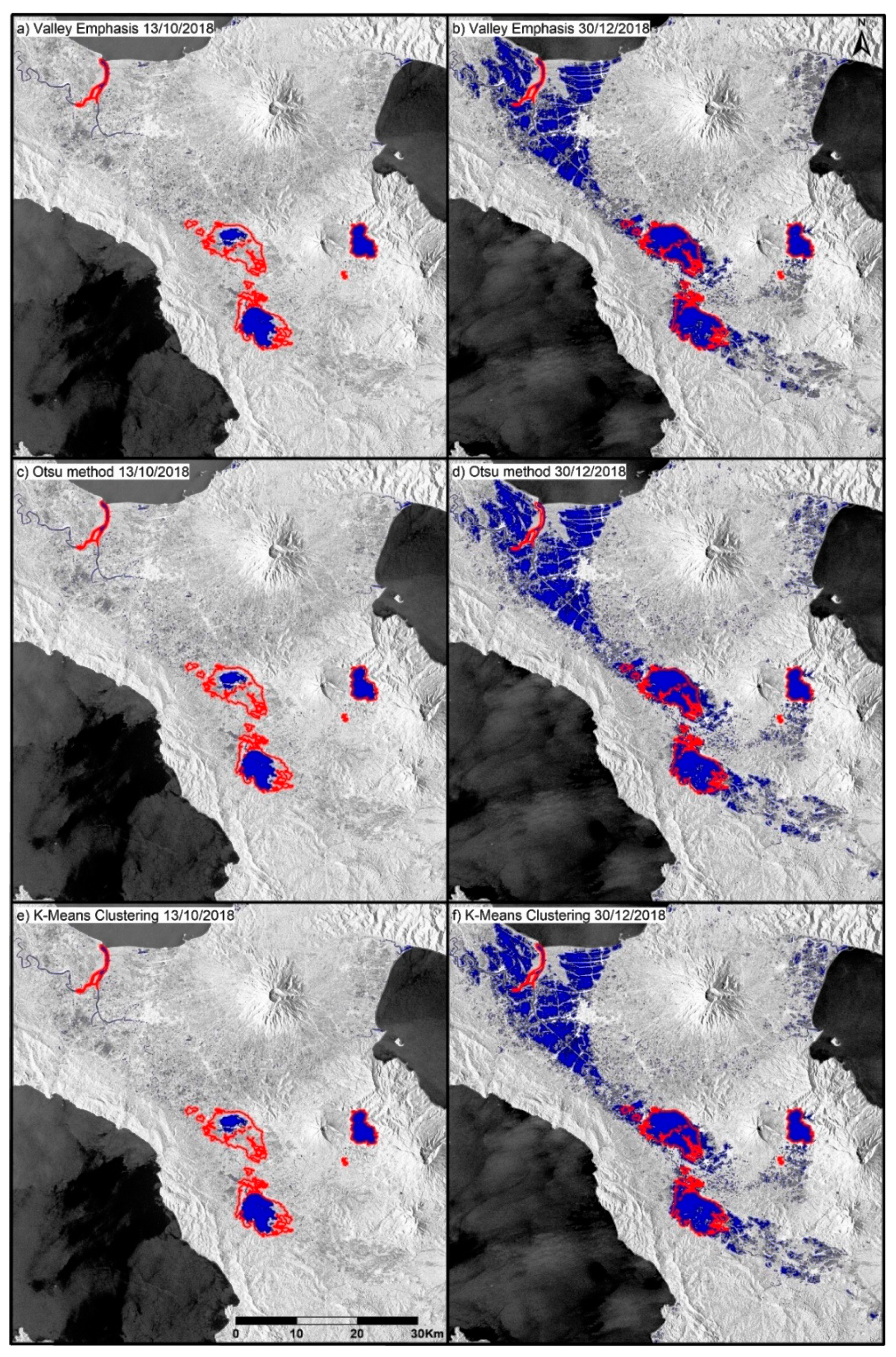
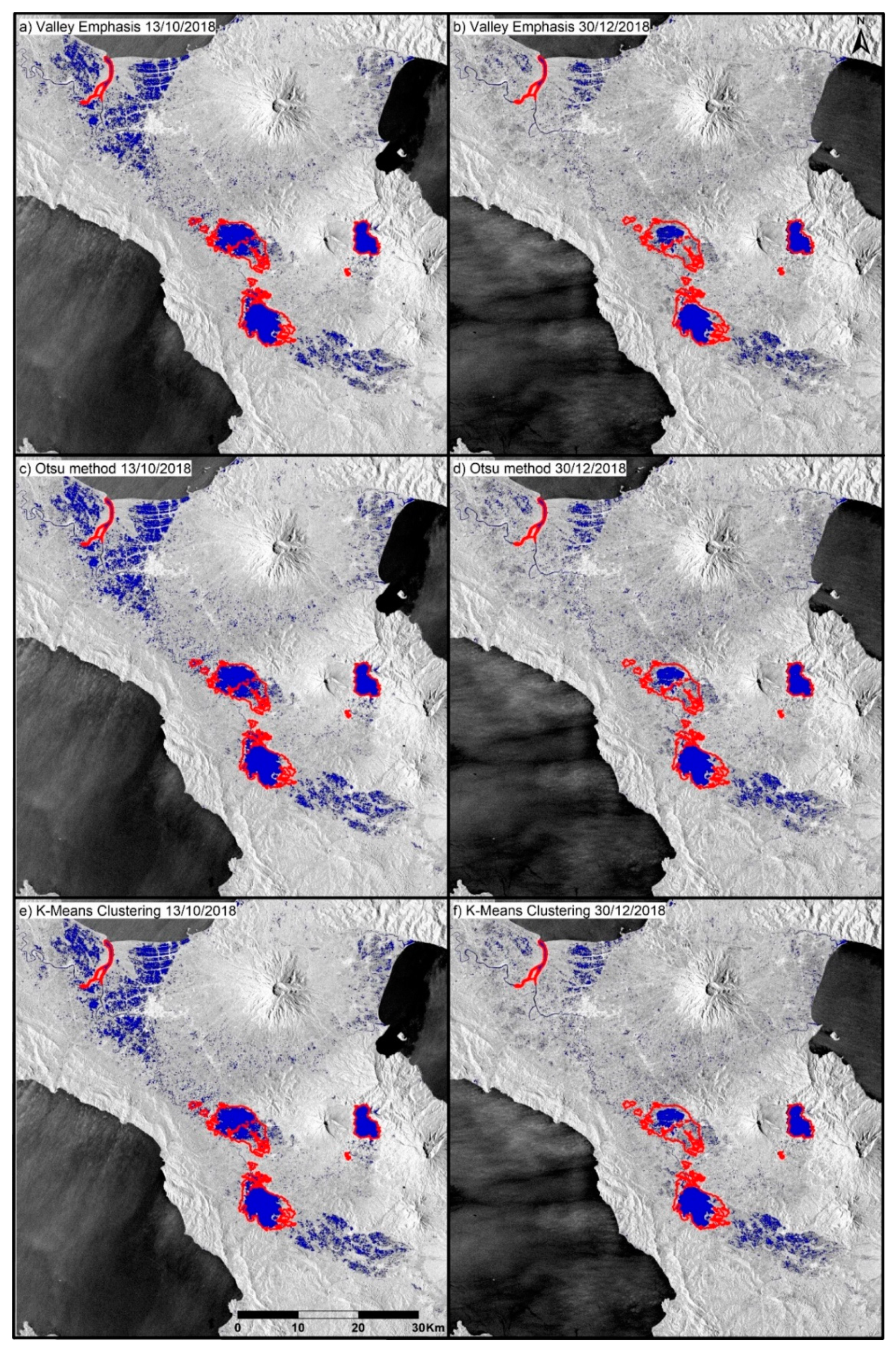
Figure 5 and Figure 6 show several examples of results in terms of open water identification from the different methods used to select the optimal threshold value of backscattering intensity. The first example reported in Figure 5a,c,e represents the water coverage at the beginning of the monitoring period before the occurrence of the rainfall events responsible for the flooding. The second example reported in Figure 5b,d,f represents the water coverage immediately after the first flood pulse induced by rainfall. Figure 6a,c,e represent the water coverage immediately after the second flood pulse induced by rainfall. The second example reported in Figure 6b,d,f represents the water coverage immediately after the third flood pulse induced by rainfall. For comparison purposes, in each map of Figure 5 and Figure 6, polygons representing water bodies as depicted in the SWBD dataset (red polygon, e.g., [65]) were overlaid with areas classified as water bodies (blue area). The SWBD is the worldwide open water bodies boundary in vector format, which were generated by the National Geospatial Intelligence Agency [66] and represent the maximum extent of open water features. A comparison of the results in terms of water coverage indicated the consistency of all of the methods across most of the study area, with local relative underestimation of the Valley Emphasis method. An example is in the northeastern sector of the study area. No differences between the Otsu and K-Means Clustering were appreciable at the scale of Figure 5 and Figure 6.
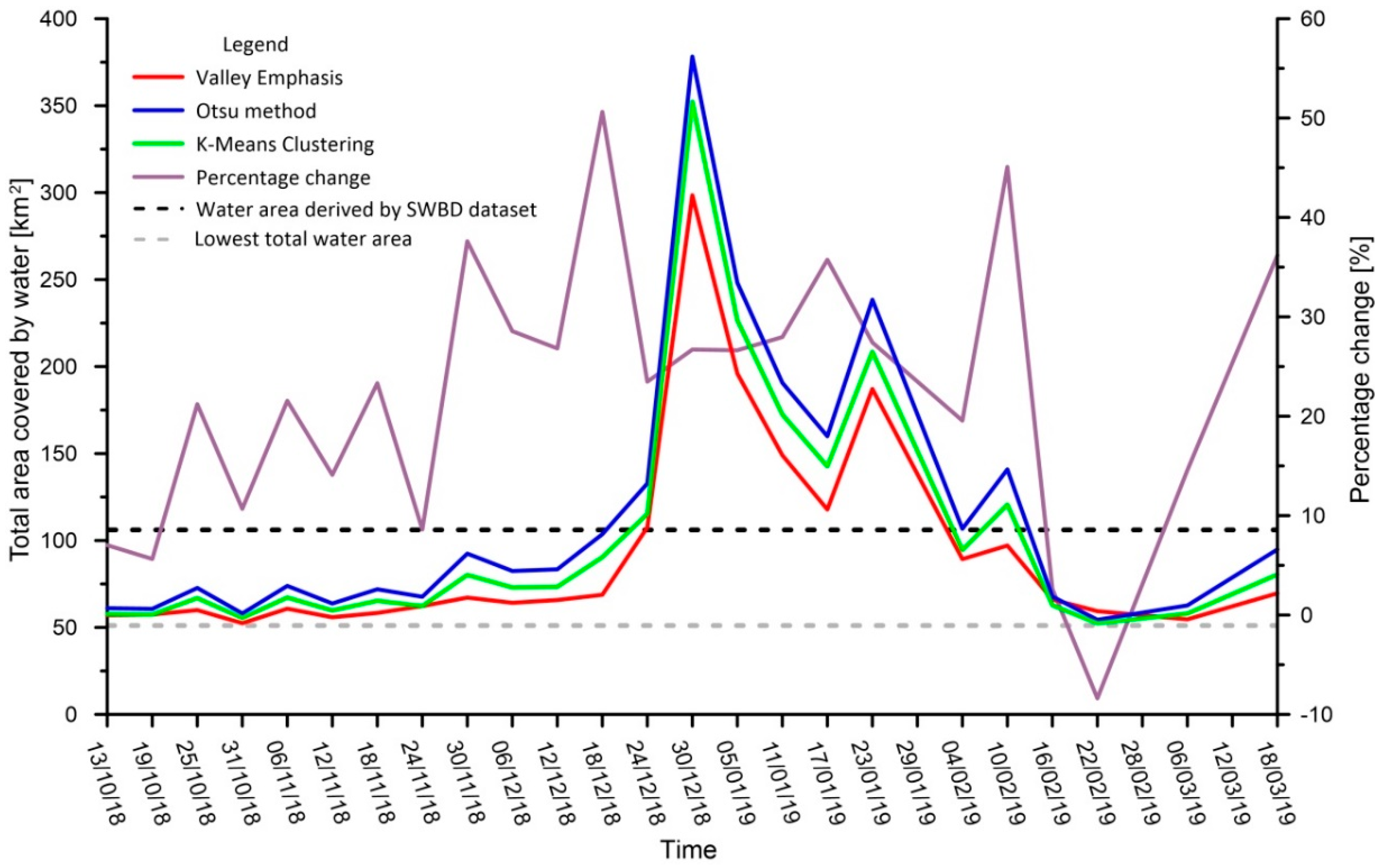
Figure 7 shows the evolution of the open water features during the period of interest, including the rainfall events responsible for multiple flood pulses, in terms of total extent for each considered method. Particularly, the red, blue, and green lines represent the total flooded area extracted by Valley Emphasis, Otsu, and K-Means Clustering methods, respectively. All three methods showed the same pattern of water coverage over time with some variable differences in terms of total estimation. Before the first flood pulse, from 13 October to 24 December the graph indicated a slow increase of water coverage, from a minimum coverage area of about 52 km2 (grey dashed line in the graph). After this first period, three individual flood pulses with decreasing intensities were identified in terms of total water area increase by our multi-method analysis. According to the PAGASA report, the first main flood pulse occurred between 30 December 2018 and 1 January 2019. A second and a third minor flood pulse followed the first occurring between 17 January 2019, and 16 February 2019. After these water surface increases, the progressive recession of open water features induced a consistent decrease of the estimated total extent of the water surface that, between 22 February 2019, and 6 March 2019, matched the extent of water features before the flood.
Even if the three methods showed consistent trends in time, a number of differences in the total estimated water area with the different methods are depicted in the graph of Figure 7. The purple line of the graph provides an overview of this change in terms of the maximum percentage change. Indeed, the average difference of approximately 20% was observable. Because of the different estimations of the open water area at the beginning of the period of interest and the absence of an official estimation, our analysis was able to provide only the relative change of the open water area coverage estimated for each different flood pulse occurring in the reference period. Notably, our analysis indicated that the first (main) flood pulse produced an increase in total water area between 245 and 326 km2, the second pulse was responsible for an increase between 135 and 186 km2, and the third event induced an increase between 45 and 88 km2. As described above and observable from the graph of Figure 7, the minimum value of open water area coverage was consistently derived by the Valley Emphasis method, while the maximum value was consistently derived by the Otsu method. The K-Means Clustering method showed water coverage values between the minimum (i.e., Valley Emphasis method) and the maximum (i.e., Otsu method). The flood-induced increases in the open water area estimated with K-Means Clustering were equal to 300, 156, and 68 km2 for the first, second, and third flood pulses, respectively. The shift from the other two methods ranged, in relative terms and considering the entire reference period, between 4% and 31%.
The Otsu method consistently showed higher open water surface values across the reference period. The tendency to overestimate water coverage by the Otsu classification method in comparison with the Valley Emphasis method was observed also by Ba Duy [59], who confirmed that this method outperformed the Otsu method in terms of absolute identification capabilities. In addition, the author of the study underlines the limitation of the Valley Emphasis method for extracting water by SAR images, including inefficient identification of mixed water pixels, confusion of water bodies with background noise, and difficulty in choosing an optimal threshold value for very large areas. Bin Cui et al. [28] indicated that conversely from threshold-based methods like the Otsu and Valley Emphasis, the unsupervised methods, like the K-Means Clustering, have great potential in the context of image classification.
The good performance of the unsupervised method in comparison with threshold-based methods can be related to its ability in capturing the spatial variability of the backscattering coefficient that represents a basis for a self-adaptation to different environmental conditions captured by SAR images. Our application confirmed that despite the lack of supervision and parameter estimation (e.g., threshold), the K-Means Clustering performed at least as good as the other methods, and possibly better than the Otsu. In this way, our interpretation is that the unsupervised methods, like the K-Means Clustering, have the potential to support SAR imagery-based flood mapping, also in long-term operational frameworks. This is also related to better results in terms of computational time [28]. It is interesting to mention that additional methods for water body classification, like Bimodal Histogram and Local Adaptive Thresholding [67], have been introduced and have the potential to support this kind of analysis. However, their applicability and reliability need to be further analyzed.
Figure 8a shows the persistence of the water in the reference period across the whole study area. In the submergence map of Figure 8a, permanent water bodies like the major lakes and the river are easily recognizable, as they are marked by a color corresponding to a value of the submergence ratio equal to 1. The Baao and Bato lakes expanded due to the flood events until they reached the boundary indicated in the SWBD dataset for a limited period of time (i.e., 20% of the reference time period). Most of the area hit by the flood stayed submerged between 5% and 25% of the time, with a number of spots in which the water persisted for approximately 40% of the reference time period. These spots were in the areas surrounding major lakes and next to the northern coastline of the study area. We expect that the temporal persistence of the flood was directly related to the water level and the presence of a draining channel.
Figure 8b–d, report the difference in the submergence ratios calculated with products derived by image classification and the selected methods. Notably, the most important differences were between submergence ratios calculated with the products derived by K-Means Clustering and Valley Emphasis based threshold definitions and between Otsu and Valley Emphasis based threshold definitions. This is consistent with the results of our analysis summarized in Figure 7.
5. Conclusions
Our analysis indicates that Sentinel-1 data have the potential to be used in flood tracking and for monsoon events characterized by long-term rainfall associated with persistent cloud coverage, which excludes the possibility of using the other types of satellite products, like optical imagery. In this study, the multi-pulse flood caused by the Usman tropical depression in the Camarines Sur Province of the Philippines was analyzed with the aim to provide quantitative flooding data and test multiple methods from a relative perspective connected to the absence of accessible official data. All of the pulses characterizing the flood event occurred between 24 December 2018, and 23 January 2019, remembered for its dramatic effects over the Camarines Sur Province, and they were detected and characterized in terms of the open total flooded area. Since the discrimination between water features and the land surface might be a very challenging task in terms of both accuracy and computation time, in our study, the open water features extraction was completed with three different methods: the Valley Emphasis based manual threshold identification, the Otsu method, and the K-Means Clustering method. All of the methods identified a shape consistent with the flooded area, with slight differences in dimensions (i.e., total area) observed over the monitoring period. These differences seem to be not correlated to the size of the total area covered by open water. Although an official estimation of the flooded area is not available, these methods provide a total flooded area that approximately averaged the results obtained with the Valley Emphasis based manual threshold identification and the Otsu method. The K-Means Clustering method is advantageous because (i) it is unsupervised, (ii) it is fully automatic, and (iii) it returned better results in terms of the computation time. A fast-computational time is a great advantage when it is necessary to have a quick overview of a flood situation. On this basis, this method might have the potential to be used in an operational flood monitoring perspective. In this framework, SAR images are an important means to study flood phenomena because of their day and night operational capabilities and their increasing frequency of acquisition related to the number of satellite constellations. In addition, these capabilities are enhanced by the free availability of data, like those derived by Sentinel-1 satellites.
Author Contributions
Conceptualization, G.R. and L.G.; methodology, G.R.; software, G.R.; validation, G.R., L.G. and G.G.; formal analysis, L.G.; investigation, G.R.; resources, P.R.; data curation, G.R. and F.M.G.; writing—original draft preparation, G.R. and L.G.; writing—review and editing, L.G., G.G., P.R. and F.M.G.; visualization, G.R.; supervision, P.R. and F.M.G.; project administration, P.R.; funding acquisition, P.R.
Funding
This research was supported by “Research University Funds” of the University of Sannio, Resp.: Paola Revellino.
Acknowledgments
We thank to two anonymous reviewers for their constructive comments.
Conflicts of Interest
The authors declare no conflict of interest.
References
- Revellino, P.; Guerriero, L.; Mascellaro, N.; Fiorillo, F.; Grelle, G.; Ruzza, G.; Guadagno, F.M. Multiple Effects of Intense Meteorological Events in the Benevento Province, Southern Italy. Water 2019, 11, 1560. [Google Scholar] [CrossRef]
- Paul, S.H.; Sharif, H.O. Analysis of Damage Caused by Hydrometeorological Disasters in Texas, 1960–2016. Geosciences 2018, 8, 384. [Google Scholar] [CrossRef]
- Ologunorisa, T.E.; Abawua, M.J. Flood risk assessment: A review. J. Appl. Sci. Eniron. Manag. 2005, 9, 57–63. [Google Scholar]
- Re, M. Natural Catastrophes 2015, Annual Figures. Munich Re NatCat Service. 2016. Available online: https://www.munichre.com/site/corporate/get/params_E1254966961_Dattachment/1130647/Munich-Re-Overview-Natural-catastrophes-2015.pdf (accessed on 9 October 2019).
- Jongman, B.; Ward, P.J.; Aerts, J.C.J.H. Global exposure to river and coastal flooding: Long term trends and changes. Glob. Environ. Chang. 2012, 22, 823–835. [Google Scholar] [CrossRef]
- Di Baldassarre, G.; Schumann, G.; Bates, P.D.; Freer, J.E.; Beven, K.J. Flood-plain mapping: A critical discussion of deterministic and probabilistic approaches. Hydrol. Sci. J. 2010, 55, 364–376. [Google Scholar] [CrossRef]
- Alfonso, L.; Mukolwem, M.M.; Di Baldassarre, G. Probabilistic flood maps to support decision-making: Mapping the value of information. Water Resour. Res. 2016, 52, 1026–1043. [Google Scholar] [CrossRef]
- Guerriero, L.; Focareta, M.; Fusco, G.; Rabuano, R.; Guadagno, F.M.; Revellino, P. Flood hazard of major river segments, Benevento Province, Southern Italy. J. Maps 2018, 14, 597–606. [Google Scholar] [CrossRef] [Green Version]
- Hoet, P.H.M.; Geys, J.; Nemmar, A.; Nemery, B. NATO Science for Peace and Security Series C, Environmental Security; Korgan, F., Powell, A., Fedorov, O., Eds.; Springer: New York, NY, USA, 2011. [Google Scholar]
- Klemas, V. Remote Sensing of Floods and Flood-Prone Areas: An Overview. J. Coast. Res. 2015, 31, 1005–1013. [Google Scholar] [CrossRef]
- Matgen, P.; Schumann, G.; Henry, J.B.; Hoffmann, L.; Pfister, L. Integration of SAR-derived river inundation areas, high-precision topographic data and a river flow model toward near real-time flood management. Int. J. Appl. Earth Obs. Geoinf. 2007, 9, 247–263. [Google Scholar] [CrossRef]
- Kussul, N.; Shelestov, A.; Shakun, S. Intelligent computations for flood monitoring. In Proceedings of the XIVth International Conference ‘Knowledge-Dialogue-Solution’ KDS, Varna, Bulgaria, 23 June–3 July 2008. [Google Scholar]
- Shen, X.; Wang, D.; Mao, K.; Anagnostu., E.; Hong, Y. Inundation Extent Mapping by Synthetic Aperture Radar a Review. Remote Sens. 2019, 11, 879. [Google Scholar] [CrossRef]
- Ban, Y.; Jacob, A.; Gamba, P. Spaceborne SAR data for global urban mapping at 30 m resolution using a robust urban extractor. ISPRS J. Photogramm. Remote Sens. 2015, 103, 28–37. [Google Scholar] [CrossRef]
- Kiage, L.M.; Walker, N.D.; Balasubramanian, S.; Baras, J. Application of Radarsat-1 synthetic aperture radar imagery to assess hurricane-related flooding of coastal Louisiana. Int. J. Remote Sens. 2005, 26, 5359–5380. [Google Scholar] [CrossRef]
- Bolanos, S.; Stiff, D.; Brisco, B.; Pietroniro, A. Operational Surface Water Detection and Monitoring Using Radarsat 2. Remote Sens. 2016, 8, 285. [Google Scholar] [CrossRef]
- Giustarini, L.; Hostache, R.; Matgen, P.; Schumann, J.-P. A Change Detection Approach to Flood Mapping in Urban Areas Using TerraSAR-X. IEEE Trans. Geosci. Remote Sens. 2013, 51, 2417–2430. [Google Scholar] [CrossRef]
- Mason, D.C.; Davenport, I.J.; Neal, J.C.; Shumann, G.J.-P.; Bates, P.D. Near real-time flood detection in urban and rural areas using high resolution synthetic aperture radar images. IEEE Trans. Geosci. Remote Sens. 2012, 50, 3041–3052. [Google Scholar] [CrossRef]
- Martinis, S.; Plank, S.; Cwik, K. The Use of Sentinel-1 Time-Series Data to Improve Flood Monitoring in Arid Areas. Remote Sens. 2018, 10, 583. [Google Scholar] [CrossRef]
- Xing, L.; Tang, X.; Wang, H.; Fan, W.; Wang, G. Monitoring monthly surface water dynamics of Dongting using Sentinel-1 data at 10 m. PeerJ 2018, 6, e4992. [Google Scholar] [CrossRef]
- Chapman, B.; McDonald, K.; Shimada, M.; Rosenqvist, A.; Schroeder, R.; Hess, L. Mapping Regional Inundation with Spaceborn L-Band SAR. Remote Sens. 2015, 7, 5440–5470. [Google Scholar] [CrossRef]
- Refice, A.; D’Addabbo, A.; Lovergine, F.P.; Tijani, K.; Morea, A.; Nutricato, R.; Bovenga, F.; Nitti, D.O. Monitoring Flood Extent and Area Through Multisensor, Multi-temporal Remote Sensing: The Strymonas (Greece) River Flood. In Flood Monitoring through Remote Sensing; Springer Remote Sensing/Photogrammetry; Springer: Cham, Switzerland, 2018. [Google Scholar] [CrossRef]
- Hakdaoui, S.; Emran, A.; Pradhan, B.; Lee, C.-W.; Fils, S.C.N. A Collaborative Change Detection Approach on Multi-Sensor Spatial Imagery for Desert Wetland Monitoring after a Flash Flood in Southern Morocco. Remote Sens. 2019, 11, 1042. [Google Scholar] [CrossRef]
- Schumann, G.J.-P.; Neal, J.C.; Mason, D.C.; Bates, P.D. The accuracy of sequential aerial photography and SAR data for observing urban flood dynamics, a case study of the UK summer 2007 floods. Remote Sens. Environ. 2011, 115, 2536–2546. [Google Scholar] [CrossRef]
- Schumann, G.; Henry, J.B.; Hoffmann, L.; Pfister, L.; Pappenberger, F.; Matgen, P. Demonstrating the high potential of remote sensing in hydraulic modelling and flood risk management. In Proceedings of the Annual Conference of the Remote Sensing and Photogrammetry Society with the NERC Earth Observation Conference, Portsmouth, UK, 6–9 September 2005. [Google Scholar]
- Psomiadis, E. Flash flood area mapping utilizing Sentinel-1 radar data. In Proceedings of the SPIE Earth Resources and Environmental Remote Sensing/GIS Applications VII, Edinburgh, UK, 26–29 September 2016; p. 100051G. [Google Scholar]
- Bioresita, F.; Puissant, A.; Stumpf, A.; Malet, J.-P. A Method for Automatic and Rapid Mapping of Water Surface from Sentinel-1 Imagery. Remote Sens. 2018, 10, 217. [Google Scholar] [CrossRef]
- Cui, B.; Zhang, Y.; Yan, L.; Wei, J.; Wu, H. An Unsupervised SAR Change Detection Method Based on Stochastic Subspace Ensemble Learning. Remote Sens. 2019, 11, 1314. [Google Scholar] [CrossRef]
- Schlaffer, S.; Matgen, P.; Hollaus, M.; Wagner, W. Flood detection from multi-temporal SAR data using harmonic analysis and change detection. Int. J. Appl. Earth Obs. Geoinf. 2015, 38, 15–24. [Google Scholar] [CrossRef]
- Bazi, Y.; Bruzzone, L.; Melgani, F. An Unsupervised Approach Based on the Generalized Gaussian Model to Automatic Change Detection in Multiple SAR Images. IEEE Trans. Geosci. Remote Sens. 2005, 43, 874–887. [Google Scholar] [CrossRef]
- Huang, W.; De Vries, B.; Huang, C.; Lang, M.W.; Jones, J.W.; Creed, I.F.; Carroll, M.L. Automated Extraction of Surface Water Extent from Sentinel-1 Data. Remote Sens. 2018, 10, 797. [Google Scholar] [CrossRef]
- Benoudjit, A.; Guida, R. A Novel Automated Mapping of the Flood Extent on SAR Images Using a Supervised Classifier. Remote Sens. 2019, 11, 779. [Google Scholar] [CrossRef]
- Nakmuenwai, P.; Yamazaki, F.; Liu, W. Automated Extraction of Inundated Areas from Multi-Temporal Dual-Polarizatio RADARSAT-2 Images of the 2011 Central Thailand Flood. Remote Sens. 2017, 9, 78. [Google Scholar] [CrossRef]
- Bayik, C.; Abdikan, S.; Ozbulak, G.; Alasang, T.; Aydemir, S.; Sanli, F.B. Exploring multi-temporal Sentinal-1 SAR data for flood extend mapping. Int. Arch. Photogramm. Remote Sens. Spatial Inf. Sci. 2018, 42, 109–113. [Google Scholar] [CrossRef]
- Martinis, S.; Kuenzer, C.; Wendleder, A.; Hult, J.; Twele, A.; Roth, A.; Dech, S. Comparing four operational SAR-based water and flood detection approaches. Int. J. Remote Sens. 2015, 36, 3519–3543. [Google Scholar] [CrossRef]
- Pajuelas, G.B. A Study of Rainfall Variations in the Philippines: 1950–1996. Sci. Diliman 2000, 12, 1–28. [Google Scholar]
- Cinco, A.T.; Hilario, D.F.; de Guzman, G.R.; Ares, D.E. Climate trends and projections in the Philippines. In Proceedings of the 12th National Convention on Statistics (NCS), Mandaluyong City, Philippines, 1–2 October 2013. [Google Scholar]
- Torres, R.; Snoeij, P.; Geudtner, D.; Bibby, D.; Davidson, M.; Attema, E.; Potin, P.; Rommen, B.; Floury, N.; Brown, M.; et al. GMES Sentinel-1 mission. Remote Sens. Environ. 2012, 120, 9–24. [Google Scholar] [CrossRef]
- Henry, J.B.; Chastanet, P.; Fellah, K.; Densos, Y.L. Envisat multipolarized ASAR for flood mapping. Int. J. Remote Sens. 2006, 27, 1921–1929. [Google Scholar] [CrossRef]
- Schumann, G.; Bates, P.D.; Horritt, M.S.; Matgen, P.; Pappenberger, F. Progress in integration of remote sensing-derived flood extent and stage data and hydraulic models. Rev. Geophys. 2009, 47, RG4001. [Google Scholar] [CrossRef]
- Brisco, B. Mapping and Monitoring Surface Water and Wetlands with Synthetic Aperture Radar. In Remote Sensing of Wetlands: Applications and Advances; Tiner, R., Lang, M., Klemas, V., Eds.; CRC Press: Boca Raton, FL, USA, 2015; pp. 119–136. [Google Scholar]
- Chini, M.; Hostache, R.; Giustarini, L.; Matgen, P.A. Hierarchical Split-Based Approach for Parametric Thresholding of SAR Images: Flood Inundation as Test Case. IEEE Trans. Geosci. Remote Sens. 2017, 55, 6975–6988. [Google Scholar] [CrossRef]
- Ulaby, F.T.; Dobson, M.C. Handbook of Radar Scattering Statistics for Terrain; Arthech House: Norwood, MA, USA, 1989; ISBN 0890063362. [Google Scholar]
- Small, D. Flattening gamma: Ratiometic terrain correction for SAR imagery. IEEE Trans. Geosci. Remote Sens. 2011, 49, 3081–3093. [Google Scholar] [CrossRef]
- Lee, J.S.; Wen, J.H.; Ainsworth, T.L.; Chen, K.-S.; Chen, A.J. Improved sigma filter for speckle filtering of SAR imagery. IEEE Trans. Geosci. Remote Sens. 2009, 47, 202–213. [Google Scholar]
- Lee, J.S.; Jurkevich, I. Speckle Filtering of Synthetic Aperture Radar Images: A review. Remote Sens. Rev. 1994, 8, 313–340. [Google Scholar] [CrossRef]
- Whoodhouse, I.H. Introduction to Microwave Remote Sensing; CRC Press: Boca Raton, FL, USA, 2017. [Google Scholar]
- Shumann, G.; Di Baldassarre, G.; Bates, P. The utility of space-borne radar to render flood inundation maps based on multialgorithm ensembles. IEEE Trans. Geosci. Remote Sens. 2009, 47, 2801–2807. [Google Scholar] [CrossRef]
- Manjusree, P.; Kumar, L.P.; Bhatt, C.M.; Rao, G.S.; Bhanumurthy, V. Optimization of threshold ranges for rapid flood inundation mapping by evaluating backscatter profiles of high incidence angle SAR Images. Int. J. Disaster Risk Sci. 2012, 3, 113–122. [Google Scholar] [CrossRef]
- Long, S.; Fatoyinbo, T.E.; Policelli, F. Flood extent mapping for Namibia using change detection and thresholding with SAR. Int. J. Environ. Res. Lett. 2012, 9, 035002. [Google Scholar] [CrossRef]
- Mason, D.C.; Speck, R.; Devereux, B.; Schumann, G.J.-P.; Neal, J.C.; Bates, P.D. Flood detection in urban areas using TerraSAR-X. IEEE Trans. Geosci. Remote Sens. 2010, 48, 882–894. [Google Scholar] [CrossRef]
- Glasbey, C. An analysis of histogram-based thresholding algorithms. CVGIP Graph. Models Image Process. 1993, 55, 532–537. [Google Scholar] [CrossRef]
- Fan, J.; Lei, B. A modified valley-emphasis method for automatic thresholding. Pattern Recogn. Lett. 2012, 33, 703–708. [Google Scholar] [CrossRef]
- Al-Bayanti, M.; El-Zaart, A. Automatic thresholding techniques for SAR images. In Proceedings of the International Conference of Soft Computing, Dubai, UAE, 2–3 November 2013. [Google Scholar]
- Martinis, S.; Twele, A.; Voigt, S. Towards operational near-real time flood detection using a split-based automatic thresholding procedure on high resolution TerraSAR-X data. Nat. Hazards Earth Syst. Sci. 2009, 9, 303–314. [Google Scholar] [CrossRef]
- Martinis, S.; Kersten, J.; Twele, A. A fully automated TerraSAR-X based flood service. ISPRS Int. J. Photogramm. Remote Sens. 2015, 104, 203–212. [Google Scholar] [CrossRef]
- Martinis, S.; Twele, A.; Strobl, C.; Kersten, J.; Stein, E. A Multi-scale flood monitoring system based on fully automatic MODIS and TerraSAR-X processing chains. Remote Sens. 2013, 104, 203–212. [Google Scholar] [CrossRef]
- Hostanche, R.; Matgen, P.; Schumann, G.; Puech, C.; Hoffmann, L.; Pfister, L. Water level estimation and reduction of hydraulic model calibration uncertainties using satellite SAR images of floods. IEEE Trans. Geosci. Remote Sens. 2009, 47, 882–894. [Google Scholar]
- Nguyen, B.D. Automatic detection of surface water bodies from Sentinel-1 SAR images using Valley-Emphasis methods. Vietnam J. Earth Sci. 2015, 37, 328–343. [Google Scholar]
- Fuang, H.; Jargalsaikhan, D.; Tsai, H.-C.; Lin, C.-Y. An Improved Method for Image Thresholding based on the Valley-Emphasis Method. In Proceedings of the Asia-Pacific Signal and Information Processing Association Annual Summit and Conference, Kaohsiung, Taiwan, 29 October–1 November 2013. [Google Scholar] [CrossRef]
- Otsu, N. A threshold selection method from gray-level histogram. IEEE Trans. Syst. Man Cybern. 1979, 9, 62–66. [Google Scholar] [CrossRef]
- Zheng, Y.; Zhang, X.; Hou, B.; Liu, G. Using Combined Difference Image and k -Means Clustering for SAR Image Change Detection. IEEE Geosci. Remote Sens. Lett. 2014, 11, 691–695. [Google Scholar] [CrossRef]
- Celik, T. Unsupervised Change Detection in Satellite Images Using Principal Component Analysis and k-Means Clustering. IEEE Geosci. Remote Sens. Lett. 2009, 6, 772–776. [Google Scholar] [CrossRef]
- Ravichandran, K.S.; Ananthi, B. Color Skin Segmentation Using K-Means Cluster. Int. J. Comput. Appl. Math. 2009, 4, 153–157. [Google Scholar]
- Santoro, M.; Wegmüller, U.; Lamarche, C.; Bontemps, S.; Defourny, P.; Arino, O. Strengths and weaknesses of multi-year Envisat ASAR backscatter measurements to map permanent open water bodies at global scale. Remote Sens. Environ. 2015, 171, 185–201. [Google Scholar] [CrossRef]
- SWBD. Shuttle Radar Topography Mission Water Body Data Set. Digital Media. 2005. Available online: https://dds.Cr.Usgs.Gov/srtm/version2_1/ (accessed on 27 July 2019).
- Gahlaut, S. Determination of Surface Water Area Using Multitemporal SAR Imagery. Master’s Thesis, University of Stuttgart, Stuttgart, Germany, 2015. [Google Scholar] [CrossRef]
Figure 1.
Map showing the study area (dashed line divides Camarines Sur and Albay provinces). The blue line indicates the major river, lakes are represented by blue polygons, towns are reported using black dots, and major reliefs are depicted by black triangles. The inset map shows the climatic regions of the study area.

Figure 2.
Examples of pre-processed Synthetic Aperture Radar (SAR) images of the study area in the period between 13 October 2018, and 11 January 2019. The dark areas represent open water features and shadow zones.
Figure 2.
Examples of pre-processed Synthetic Aperture Radar (SAR) images of the study area in the period between 13 October 2018, and 11 January 2019. The dark areas represent open water features and shadow zones.

Figure 3.
Examples of pre-processed SAR images of the study area in the period between 17 January 2019, and 22 February 2019. The dark areas represent open water features and shadow zones.
Figure 3.
Examples of pre-processed SAR images of the study area in the period between 17 January 2019, and 22 February 2019. The dark areas represent open water features and shadow zones.

Figure 4.
Processing workflow of SAR imagery for estimating the total surface covered by water across the study area in the reference period.
Figure 4.
Processing workflow of SAR imagery for estimating the total surface covered by water across the study area in the reference period.

Figure 5.
Examples of results in terms of open water extent obtained by multiple methods. Blue areas represent the extracted open water features, and red polygons represent SWBD water body boundaries. (a,c,e) represent the extent of open water features before the rainfall events responsible for the flooding. (b,d,f) represent the extent of open water features after the first flood pulse (main).

Figure 6.
Examples of results in terms of open water extent obtained by multiple methods. Blue areas represent the extracted open water features, and red polygons represent SWBD water body boundaries. (a,c,e) represent the extent of open water features after the second rainfall event responsible for the flooding. (b,d,f) represent the extent of open water features after the third flood pulse.

Figure 7.
Graph showing the evolution of open water feature surface coverage estimated with the Valley Emphasis, Otsu, and K-Means Clustering methods (i.e., red, blue and green lines, respectively) in the study area over the monitoring period. The purple line shows the percentage difference of water area between the Valley Emphasis and Otsu methods, which show the lowest and the highest estimation value. The gray line represents the minimum value of the water area estimated by our analysis before the occurrence of the flood, and the black line represents the water area derived by the SWBD dataset.

Figure 8.
The map of (a) shows the submergence ratio (i.e., the flood persistence) in the reference period. A pixel value equal to 1 corresponds to an always flooded area. A value of 0 corresponds to a never flooded area. The maps of (b–d) are the differences in submergence ratios calculated using open water features extracted by different methods.

© 2019 by the authors. Licensee MDPI, Basel, Switzerland. This article is an open access article distributed under the terms and conditions of the Creative Commons Attribution (CC BY) license (http://creativecommons.org/licenses/by/4.0/).
Share and Cite
MDPI and ACS Style
Ruzza, G.; Guerriero, L.; Grelle, G.; Guadagno, F.M.; Revellino, P. Multi-Method Tracking of Monsoon Floods Using Sentinel-1 Imagery. Water 2019, 11, 2289. https://doi.org/10.3390/w11112289
AMA Style
Ruzza G, Guerriero L, Grelle G, Guadagno FM, Revellino P. Multi-Method Tracking of Monsoon Floods Using Sentinel-1 Imagery. Water. 2019; 11(11):2289. https://doi.org/10.3390/w11112289
Chicago/Turabian StyleRuzza, Giuseppe, Luigi Guerriero, Gerardo Grelle, Francesco Maria Guadagno, and Paola Revellino. 2019. "Multi-Method Tracking of Monsoon Floods Using Sentinel-1 Imagery" Water 11, no. 11: 2289. https://doi.org/10.3390/w11112289
Note that from the first issue of 2016, this journal uses article numbers instead of page numbers. See further details here.