Numerical Prediction of Background Buildup of Salinity Due to Desalination Brine Discharges into the Northern Arabian Gulf

Abstract

Brine discharges from desalination plants into low-flushing water bodies are challenging from the point of view of dilution, because of the possibility of background buildup effects that decrease the overall achievable dilution. To illustrate the background buildup effect, this paper uses the Arabian (Persian) Gulf, a shallow, reverse tidal estuary with only one outlet available for exchange flow. While desalination does not significantly affect the long-term average Gulf-wide salinity, due to the mitigating effect of the Indian Ocean Surface Water inflow, its resulting elevated salinities, as well as elevated concentrations of possible contaminants (such as heavy metals and organophosphates), can affect marine environments on a local and regional scale. To analyze the potential effect of background salinity buildup on dilutions achievable from discharge locations in the northern Gulf, a 3-dimensional hydrodynamic model (Delft3D) was used to simulate brine discharges from a single hypothetical source location along the Kuwaiti shoreline, about 900 km from the Strait of Hormuz. Using nested grids with a horizontal resolution, comparable to a local tidal excursion (250 m), far field dilutions of about 28 were computed for this discharge location. With this far field dilution, to achieve a total dilution of 20, the near field dilution (achievable using a submerged diffuser) would need to be increased to approximately 70. Conversely, the background build-up means that a near field dilution of 20 yields a total dilution of only about 12.

1. Introduction

Marine impacts associated with brine discharge are mainly judged on their brine and contaminant concentrations after initial mixing (dilution). Dilution is generally obtained through judicious choice of outfall parameters, including location, orientation, number of ports, discharge flow rate, etc., using a combination of analytical and physical models.

The effectiveness of any discharge design will depend on the relative magnitude of the near and far field dilution. In general, the near field is facilitated by turbulent entrainment processes, while the far field is dominated by advection and diffusion processes.

The far field dilution is defined as:

S_F = (c_o − c_a)/(c_F − c_a),

(1)

where c_o, c_a, and c_F are the pollutant concentrations in the discharge, the ambient (water not influenced by the discharge) and the far field (region >~100 meters surrounding the discharge), and the near field dilution is defined as:

S_N = (c_o − c_F)/(c_N − c_F),

(2)

where c_N is the concentration in the near field (<~100 meters from the source). The combined or total local dilution at a given location, defined as:

S_T = (c_o − c_a)/(c_N − c_a),

(3)

can be obtained algebraically by combining Equations (1)–(3) to obtain:

$$\frac{1}{S_T}=\frac{1}{S_N}+\frac{1}{S_F}-\frac{1}{S_N{S}_F}\cong \frac{1}{S_N}+\frac{1}{S_F},$$

(4)

or approximately the harmonic sum of S_N and S_F. In addition, over time, it is useful to calculate a harmonic mean far field dilution (after [1,2]), which is equivalent to the arithmetic mean concentration:

$$S_{F,h}=\frac{n}{{{\displaystyle \sum }}_n\frac{1}{S_i}}.$$

(5)

While recent numerical efforts and computational advances have been able to refine the horizontal resolution to 10s of meters (and, therefore, reduce the distance between the near and far field), multiport diffusers with port diameters on the order of 10 cm would require resolutions of sub-meter level resolution, plus additional physics (e.g., entrainment, bubble dynamics or stratification) to properly model the near field mixing processes [3]. It is therefore more computationally economical to adopt two separate models to model the near and far field models and to couple them, to yield an overall dilution that is of interest [4,5].

The primary objective of this paper is to investigate the potential background buildup of a low-flushing water body on a local scale. It begins with a brief description of the oceanographic conditions of the paper’s focus area, the Arabian or Persian Gulf (hereafter referred to as the Gulf—a body of water with the potential of increased background buildup), and an analysis of long-term Gulf-wide salinity changes, due to desalination. The study considers a single hypothetical desalination brine discharge, located in the northern Gulf, and present predicted far field dilutions, using a Gulf-wide hydrodynamic model (Delft3D). The paper discusses the importance of the grid resolution, in order to resolve the background buildup concentrations, as well as illustrate tradeoffs which occur when the current fields are not well resolved. Finally, although this paper does not directly provide a diffuser outfall design, it will discuss the impact of the predicted background buildup on the target dilutions, that would need to be accomplished when designing a diffuser outfall.

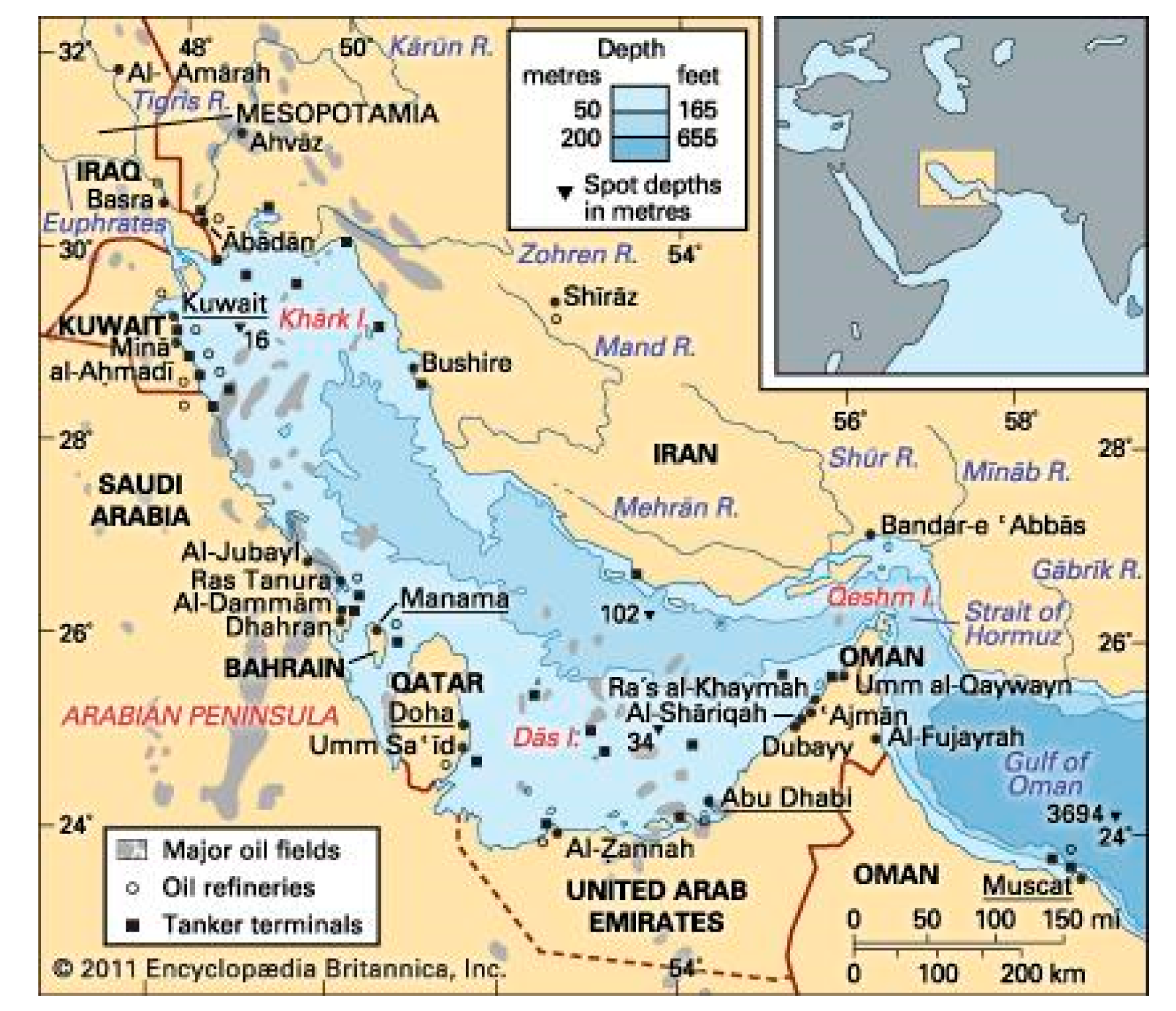
1.1. Case Study: Gulf Scale Environmental Impact

The Gulf is a shallow (mean depth of about 35 m), reverse tidal estuary, with only one outlet available for exchange flow (the Strait of Hormuz), located roughly 1000 km downcoast from the head of the Gulf. It has a minimum width of about 65 km, a maximum width of about 340 km, maximum length of about 990 km, total surface area of 239,000 km², and a total volume of about 9000 km³ [6,7] (Figure 1).

The Gulf consistently carries about a third of the world’s total seawater and brackish water desalination capacity [8,9]. Desalination has been conducted predominantly via multi-stage flash distillation (MSF) technology since the 1950s, and, due to the heat energy required, this has always been an energy intensive process. MSF plants were often located near power stations, to take advantage of the pre-heated water from the power plants’ cooling water stream as feed water for the MSF plant, in order to reduce the overall energy cost of the desalination process. In recent decades, reverse osmosis (RO) has been adopted, because of the reduced cost of desalination and its scalability (it may be implemented for individual buildings up to the largest plant, e.g., Ashkelon, Israel, with a capacity of 320,000 m³/day) [10].

Brine discharges from reverse osmosis (RO) desalination plants, located mostly throughout the Arabian coast, can contain excess salinity (up to 35,000 ppm greater than ambient), contaminants, such as heavy metals and organophosphates [9,11]. Discharges from multistage flash desalination plants additionally have an excess temperature, in the range of about 5–15 degrees Celsius warmer than ambient seawater [9].

Several studies on Gulf-wide circulation patterns exist in the literature [6,7,12,13,14,15,16,17,18,19]. This paper focuses on the drivers of the Gulf-wide circulation that are responsible for observed residual currents at a given location in the northern Gulf. The following section presents the spatial, seasonal and long-term trends in Gulf-wide salinity, which contribute to overall circulation patterns in the Gulf.

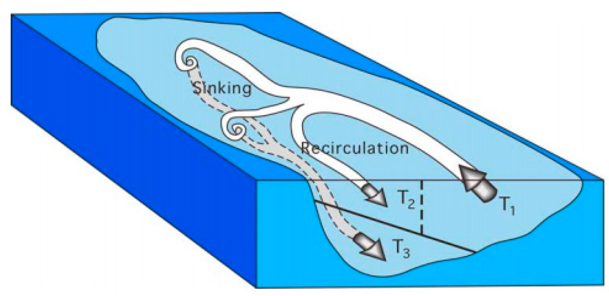
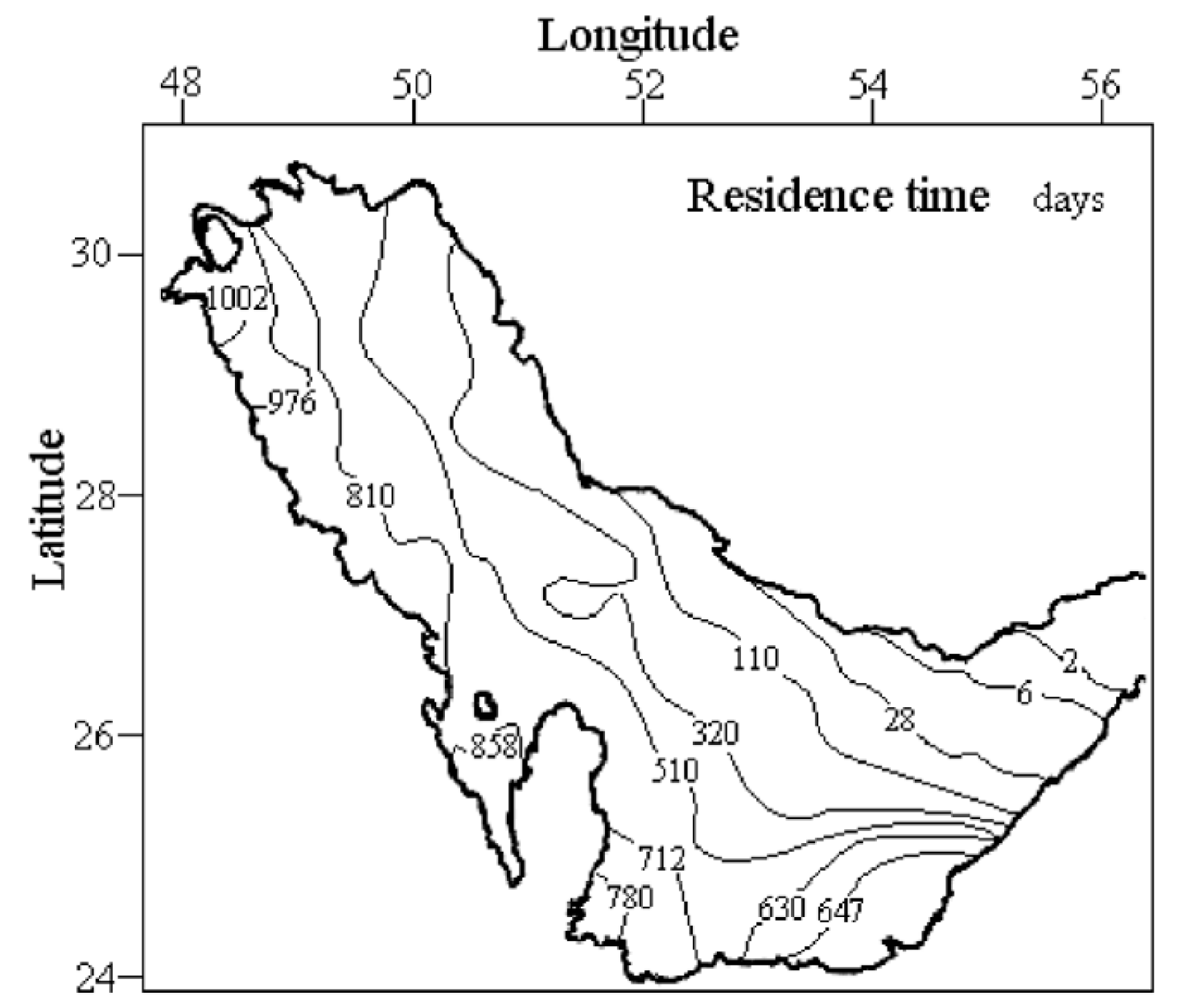
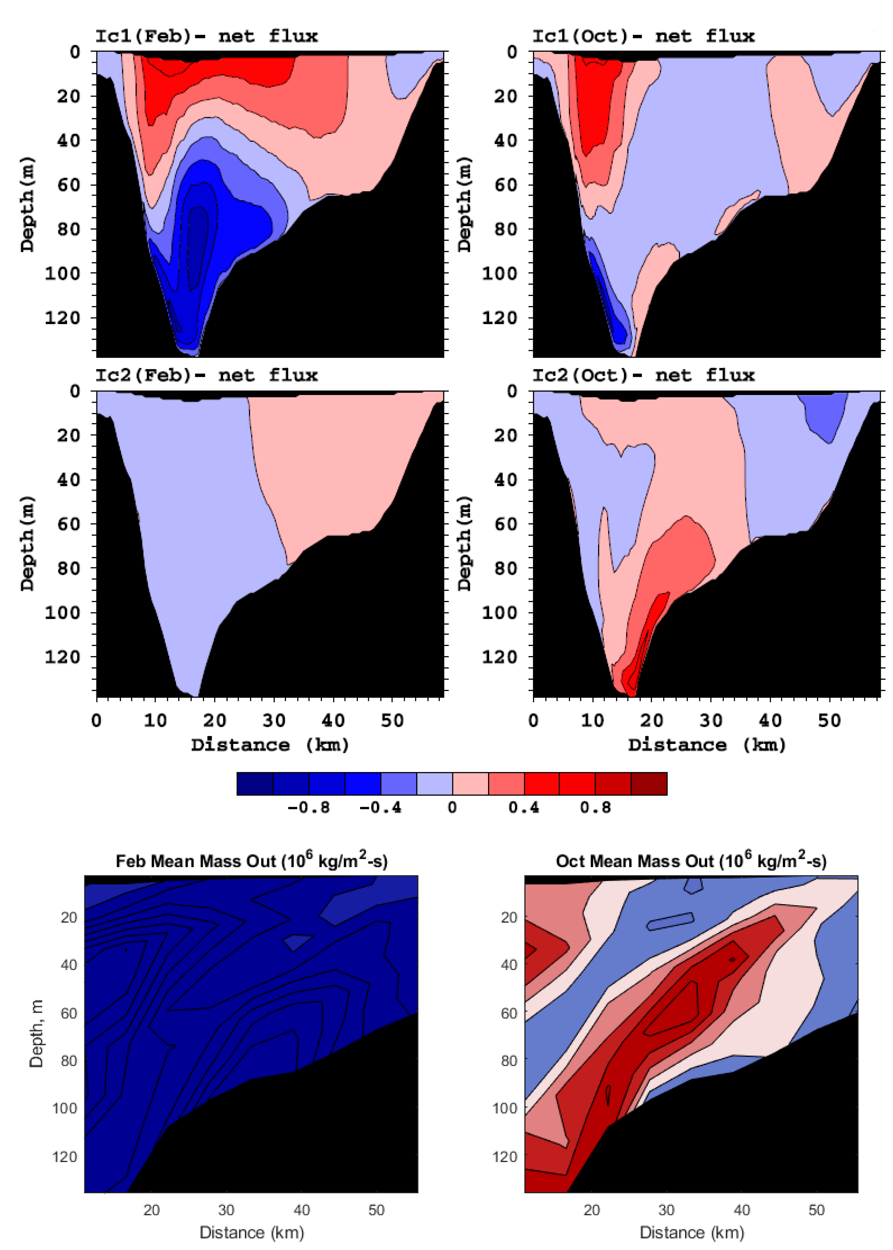
1.2. Gulf-Wide Circulation

The qualitative description of the circulation pattern in the Arabian Gulf presented here is based on field observations by Reynolds, 1993 and Johns et al. 2003 [6,7]. The Gulf itself is shallower near the Arabian coast (typically only about 20 m depth) and the Gulf deepens into a trough that runs parallel to the Iranian coast in the north. The bathymetry of the Gulf is very shallow in the southern portion, with typical bottom slopes of about 4 m over 10 km.

The circulation in the Gulf is dominated by the exchange flows in and out of the Strait of Hormuz—see Figure 2. A lower salinity surface current, known as the Indian Ocean Surface Water (IOSW), flows into the Gulf year-round (T₁ in Figure 2), initially flowing northward along the Iranian coast. While a small part of the surface current flows back out along the southern part of the Strait (shown as T₂ in Figure 2), the bulk of the flow intrudes into the Gulf, and mixes with the existing hypersaline water in the Gulf [7]. The prevailing wind, called the Shamal, is from the Northwest, and can have velocities of up to 18 m/s in the winter, compared with less than 10 m/s in the summer [13]. Additionally, the Northern Gulf receives freshwater river inflows along the Iranian coast and at the Shatt al-Arab, which contributes to circulation (with two branches of freshwater flowing southward along the Arabian and Iranian coasts). The intense evaporation of the shallow water from the Northern Gulf and the UAE coast creates a dense brine that spills into the trough to the north and leaves the Strait as a subsurface gravity current (shown as T₃ in Figure 2).

Throughout the Gulf, the tide and wind induce shear that is responsible for the dispersion of tracers. Residence times, calculated by Alosairi et al. 2011 [16], for tracer sources within the Gulf, are depicted in Figure 3. Tracer sources in shallow regions of the Arabian coast (e.g., Kuwaiti coast, Bahrain and UAE coasts) may experience residence times of 2 to 3 yrs.

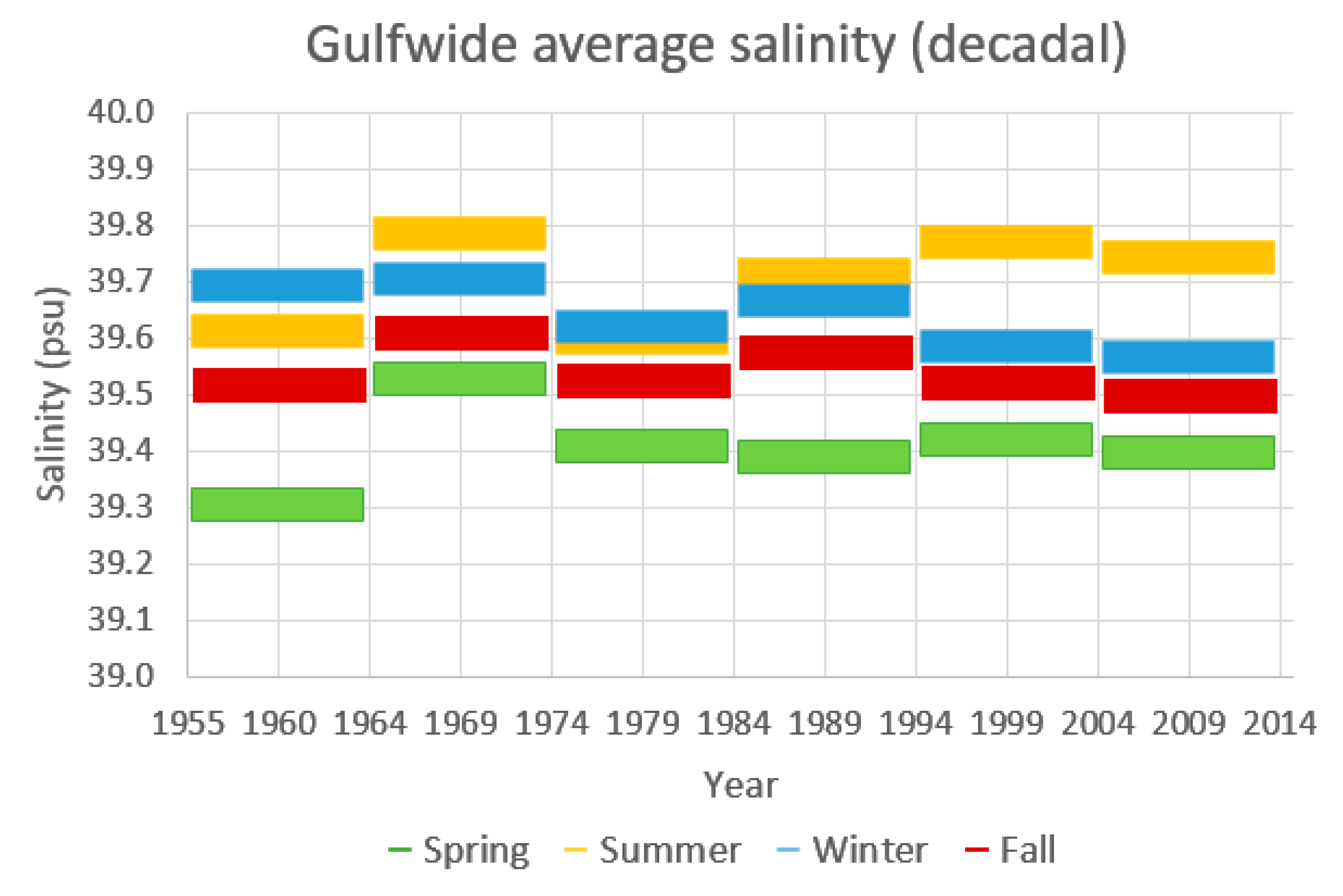
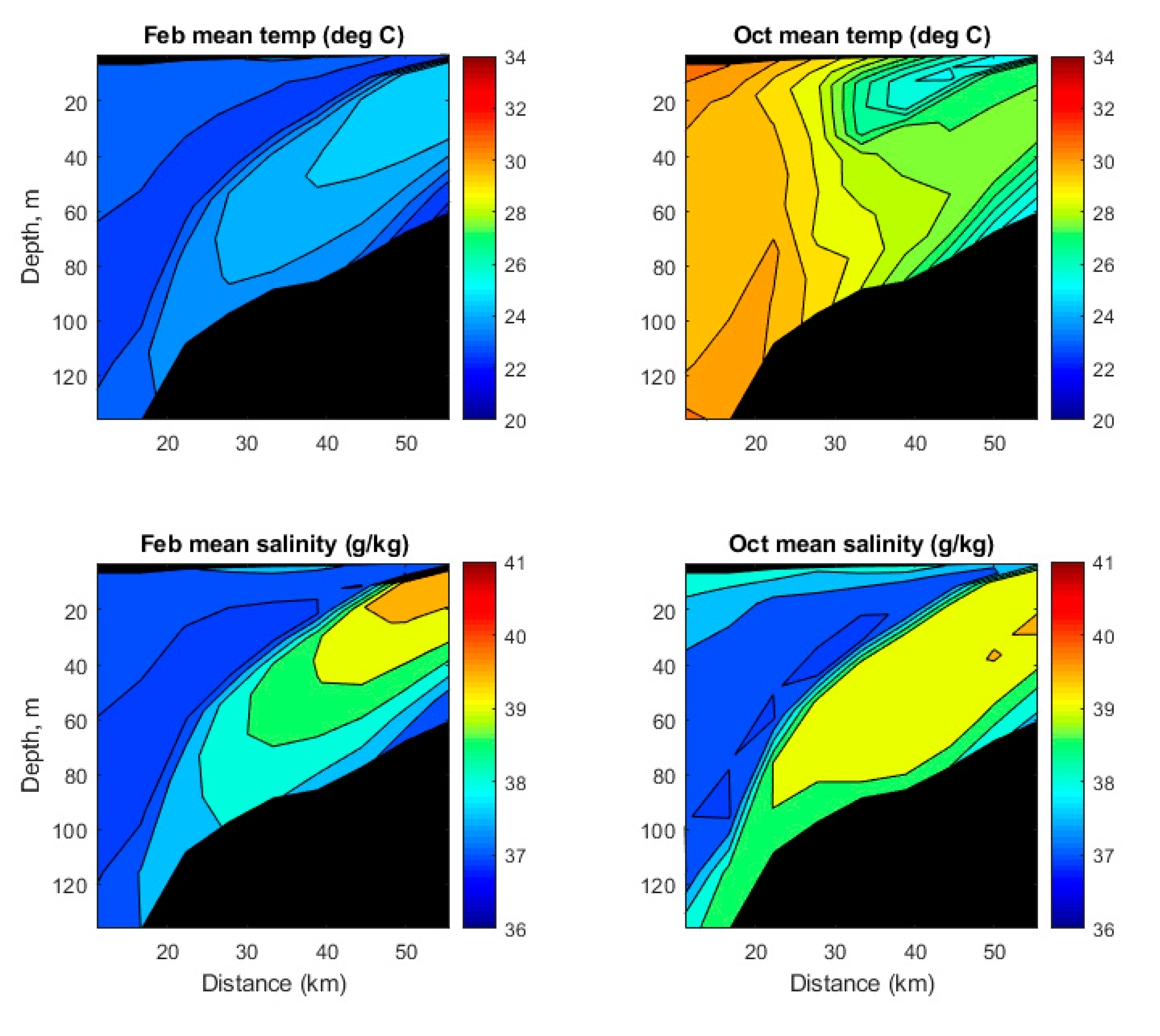
1.3. Gulf-Wide Salinity

Xue and Eltahir, 2015 [21] provided estimates of the Gulf water balance, expressed as a Gulf-averaged precipitation rate (

Table 1. Gulf water balance (Based on [21]).

Flow	Annual Flow (Expressed as Equivalent Gulf-Wide Precipitation Rate, m/yr)
Inflow through the Strait of Hormuz	+33.7 m/yr
Outflow through the Strait of Hormuz	−32.1 m/yr
Evaporation	observed −1.4 to −2.1 m/yr, model estimated −1.8 m/yr
River inflow	+0.2 m/yr
Rainfall	observed +0.07 to +0.15 m/yr, model estimated +0.09 m/yr
Desalination	up to −0.04 m/yr (may be smaller in magnitude, due to the return of some of the freshwater back into the Gulf after domestic/industrial use) [22]

):

As seen above, on a basin-wide basis, desalination amounts to an equivalent of about 2% of the evaporative loss of freshwater from the Gulf, and thus is not a major contributor to freshwater loss or increased salinity. The salinity of the Gulf is typically about 38–42 practical salinity units (psu), and it is clear from the water balance above that the high salinity of the Gulf is due to its large evaporation output compared with river and rain inputs.

Salinity values taken at different locations over the Gulf over the period 1955–2012 were obtained from the World Ocean Atlas ([19]; statistical mean of temperature on 1/4° grid). Figure 4 shows that the interdecadal variability of the salinity in the Gulf is less than the seasonal variability. The lack of variability over the decades could be attributed to the mitigating effect of the fresher inflows from the Indian Ocean via the Hormuz strait, as confirmed by modeling studies on Gulf equilibria conditions by Ibrahim, 2017 [19]. As observed on a smaller scale between two bodies of water of differing density, separated by a narrow slot (analogous to the narrow Hormuz strait) [23], the larger the density difference between the two water bodies, the larger the magnitude of the mitigating exchange flow.

2. Materials and Methods

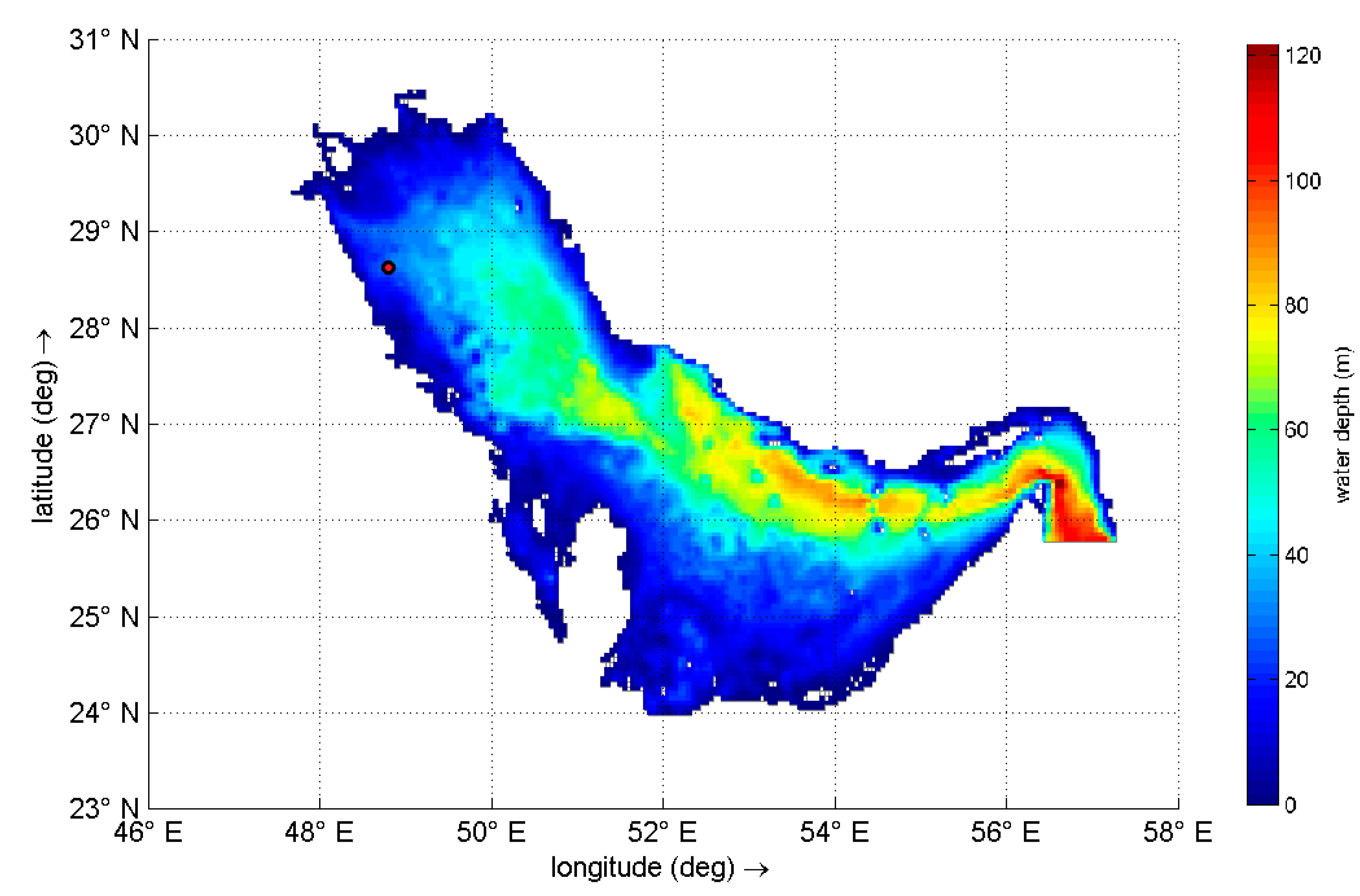
Delft3D Model

This paper used a 3-dimensional finite difference hydrodynamic model, coupled with a water quality module (Delft3D-FLOW) [25,26], as a tool to determine the far field dilution of various contaminants, as well as to quantify a background far field concentration that may affect near field outfalls. The basis for this model was the Gulf Community Model (see www.agmcommunity.org), which has been adjusted for use in the current study. A combination of measured bathymetry data, meteorological and tidal forcings, as well as freshwater riverine inflows into the Gulf, were input into the model to simulate circulation patterns in the Gulf. Details of the model are presented below.

The basic Arabian Gulf Model used a 4 km square grid (lat/lon) plus 10 vertical sigma layers (Figure 5). Our model used a 4-year hydrodynamic spin-up with a time step of 5 minutes, because contaminants discharged at Kuwait Bay may take 3 years to exit the Gulf. External forcings include gridded wind and meteorological data, and four river inputs. Tidal forcings (expressed as a time series of water elevations) were imposed along the external boundary, a transect across the Gulf of Oman in the southeastern edge of the domain (shown in Figure 5). A bottom roughness (Manning’s coefficient n = 0.03) was used throughout the Gulf.

3. Results

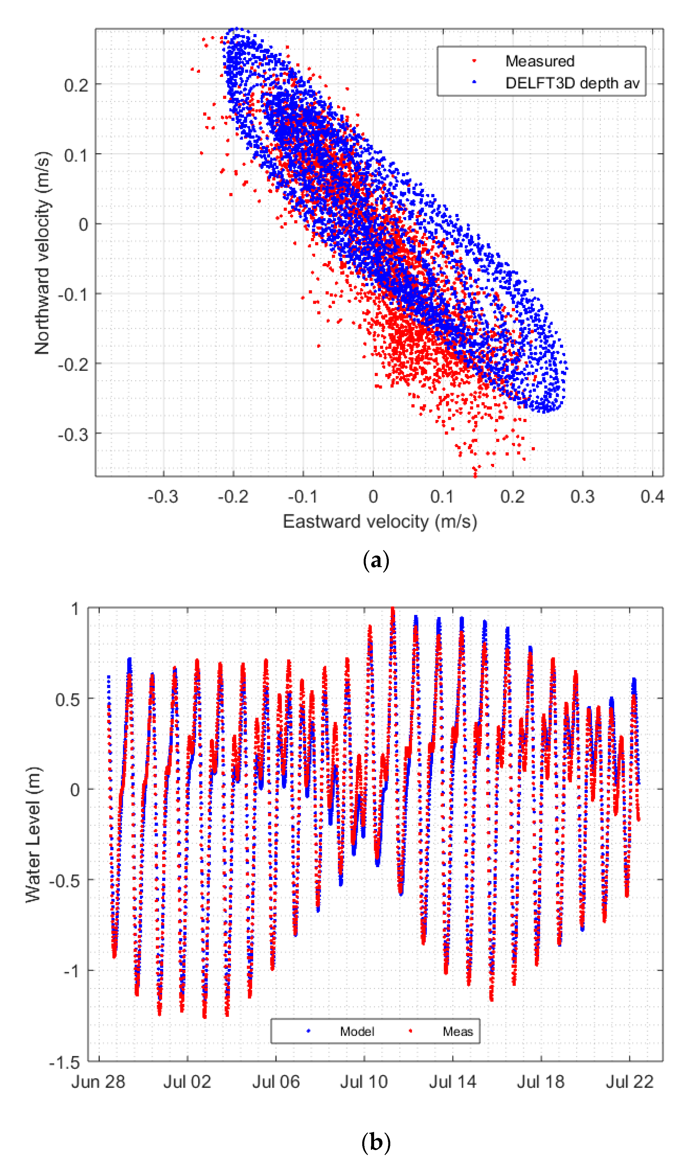
3.1. Current Speed Calibration

As the study focuses on the northern Arabian Gulf, close to Kuwaiti waters, the modeled velocity was compared with available water elevation time series at one grid cell location (Umm al Maradim Island) with Acoustic Doppler Current Profiler (ADCP) measurements provided by the Kuwait Institute of Scientific Research (KISR), during the summer of 2011, for a location ~25 km offshore and ~90 km south of Kuwait City; 28°40.153′ N, 48°38.760′ E, [25]. This data provided a sense of the tidal conditions present near the Southern Kuwaiti shore, as well as data for model calibration. Figure 6 shows a good comparison between the measured current speeds (eastward and northward) and the Delft3D modeled speeds. The observed current is mainly tidal in the southeast and northwest directions, consistent with the shore parallel direction. There is also a mean residual current of 4 cm/s in the south–southeast direction (bearing about 170 degrees). As shown in Figure 6, there is a slight mismatch in the orientation of the currents, which could be a result of the current meter’s location near an island (of dimension 800 by 300 m), whose bathymetry may not be resolved from the available depth data and model grid resolution (250 m).

While monthly data were available for some dissolved chemicals (KEPA, personal communication, 2017) for about 13 onshore and offshore locations, the time resolutions (one reading a month) are insufficient to be useful for purposes of model calibration or validation. Additionally, the monitoring locations may experience contaminants originating from multiple sources along the Kuwaiti coastline, which again cannot be resolved with the space and time resolutions available. The model calibration, using tidal data, is discussed in the section below.

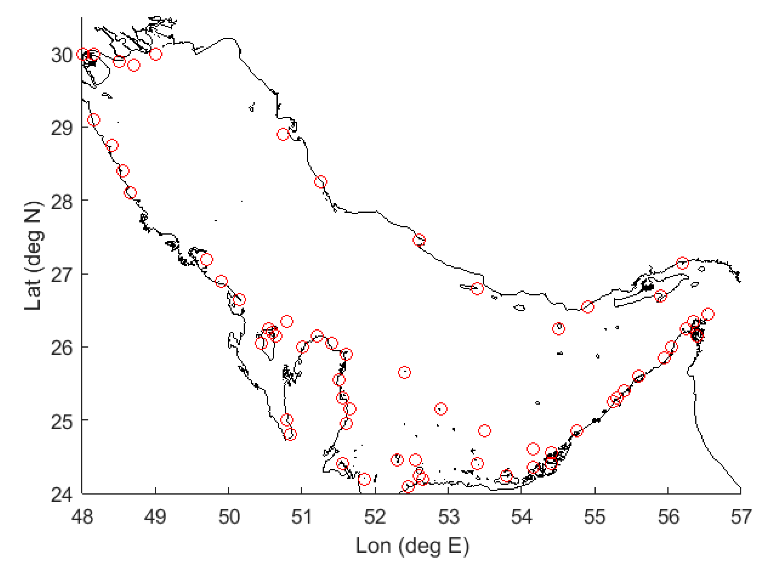
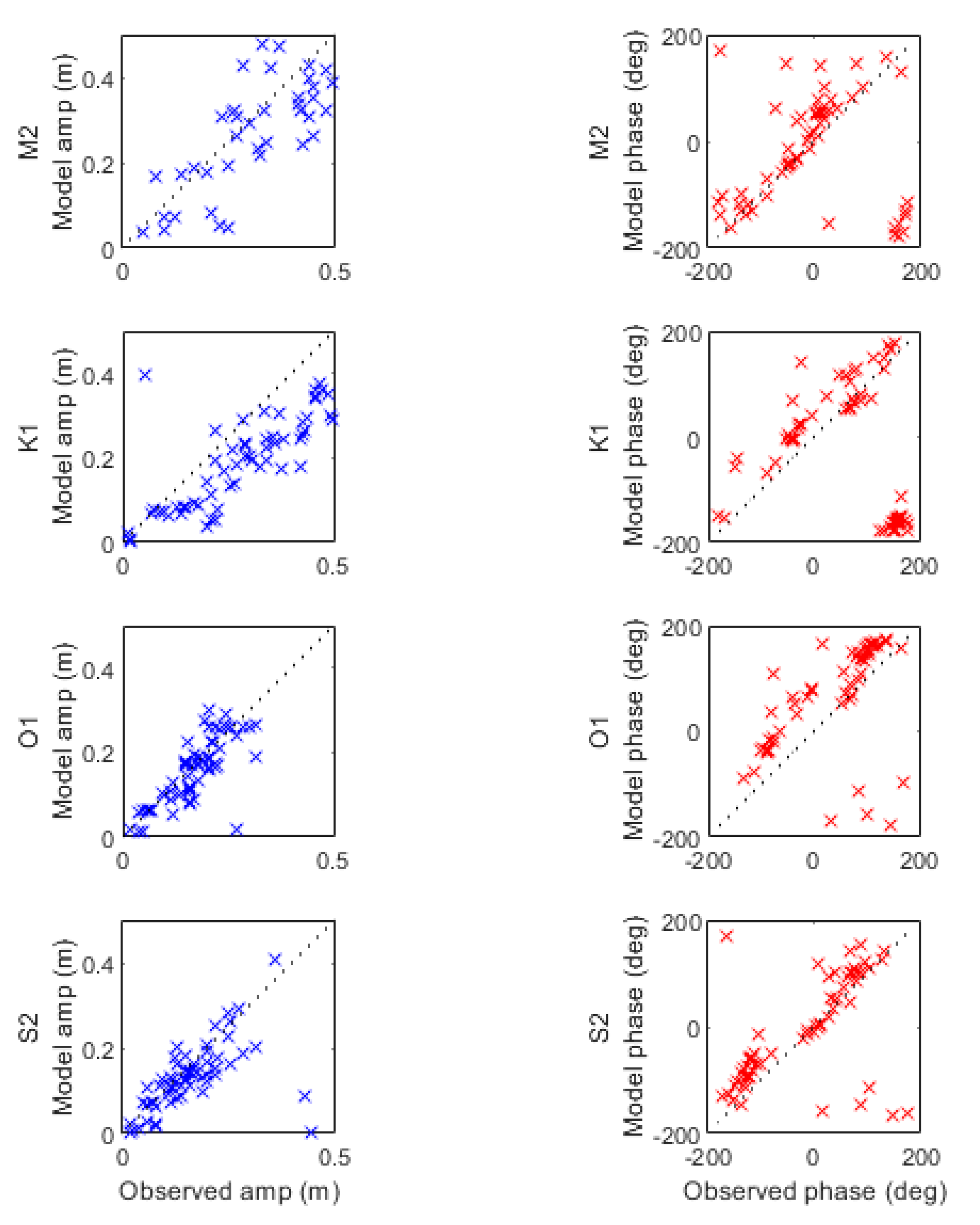
3.2. Tidal Response Calibration

While matching current speeds is an important aspect of calibration, it is also important for the model to match the tidal response at the Gulf scale. Figure 7 shows the locations in the Gulf with tidal gage data available as harmonic components. Figure 8 shows the correlation plots of M2, K1, O1, and S2 tidal components for amplitude and phases, compared with those modeled by the calibrated Delft3D model. These show that the Gulf-wide Manning’s friction coefficient of = 0.03 has resulted in good agreement with the Gulf-wide tidal amplitudes, The Gulf-wide modeled and observed tidal phases were mostly in agreement.

3.3. Hormuz Strait Calibration

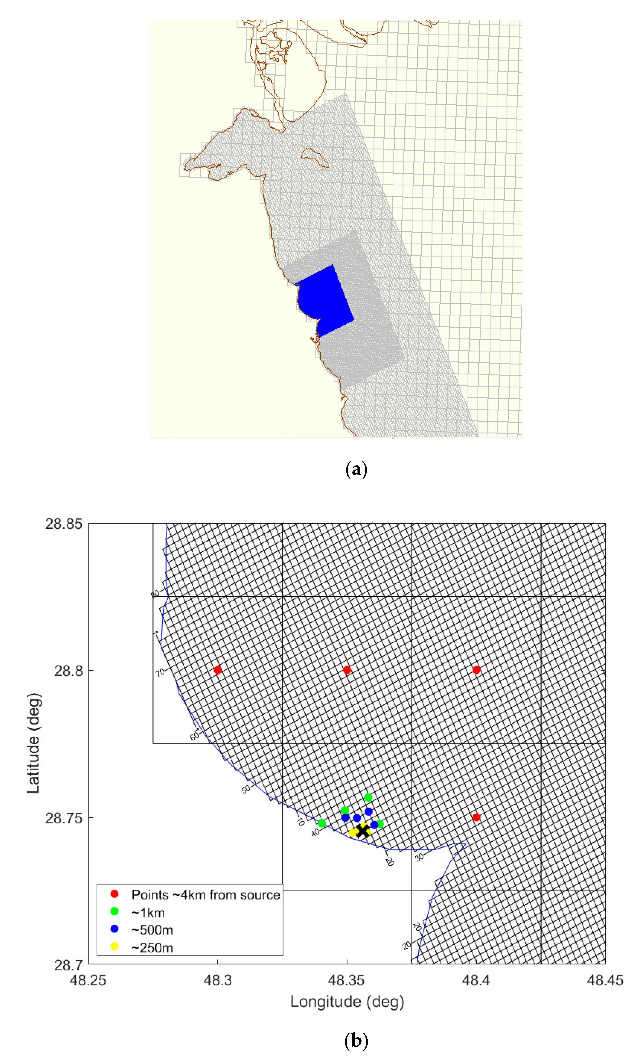
The Delft3D model was run for the entire year of 2010, and was used to compute temperature and salinity along the cross section (Figure 9), as well as the flux out of the Hormuz Strait, at different months (Figure 10). Figure 10 compared the model results with those predicted by [19], using another numeric model, FVCOM. The behavior shown in Figure 9 and Figure 10 corroborates with the qualitative circulation behavior reported by [8], namely: (1) the increased salinity stratification, coupled with influx of fresher water into the Gulf during February, and (2) the outflow of saltier water along the surface, as well as in the deeper part of the strait, in October (consistent with the flow pattern shown in Figure 2).

3.4. Nested Models

The calibrated Delft3D model was used to investigate the effect of horizontal grid resolution on the predicted far field dilution near a hypothetical brine discharge, located close to the Al-Zour power plant (a source of desalination brine). The location was chosen as it was a coastal region, close to the current meter data; similarly, the model time period matched that of current meter observations (March 2010). Figure 11a shows the inner nested model grids, in relation to the outer model. The model’s horizontal resolution was increased in the area offshore of the southern coast of Kuwait, based on the description of potential adverse effects to the marine environment, shown in Figure 11a, below. The three nested grid levels used were as follows:

• Outer = ~4 km grid (0.05 degrees)—entire Gulf
• Mid = ~1 km grid (0.01 degrees), offshore of Kuwait to ~40 km
• Fine = ~500 m grid (0.005 degrees), offshore of Kuwait to ~25 km
• Finest = 250 m grid (0.0025 degrees), offshore to Kuwait to ~10 km

Using the model results from the three nested grids, it is possible to test the mesh sensitivity of the computed dilution, resulting from a source shown in Figure 11b. To do this, model-predicted concentration timeseries were obtained for the following locations (shown in Figure 11b):

• Locations ~4 km away (horizontal grid resolution of the outer model), shown in red;
• Locations ~1 km away (resolution of the mid-scale model), shown in green;
• Locations ~500 m away (resolution of the fine model), shown in blue; and
• Locations ~250 m away (resolution of the finest model), shown in yellow.

Table 2. Harmonic mean dilutions, computed at locations at varying distances from the source, indicated in Figure 11b. Values in grey shading indicate spatially interpolated harmonic mean dilution values.

	Test Locations ~4km from Source	Test Locations ~1km from Source	Test Locations ~0.5km from Source	Test Locations ~0.25km from Source
Outer model (0.05 deg, ~4km)	2869, 3505, 2936, 4090	2902, 2879, 2879, 2879	2864, 2868, 2871, 2856	2855, 2855, 2856, 2846, 2846
Mid model (0.01 deg, ~1km)	4256, 3569, 2960, 852	189, 156, 194, 106	93, 94, 117, 94	67, 68, 77, 70, 62
Fine model (0.005 deg, ~500m)	12555, 311, 8138, 566	331, 311, 893, 158	151, 124, 218, 92	62, 63, 71, 52, 42
Finest model (0.0025 deg, ~250m)	13237, 609, 7726, 557	286, 609, 1311, 160	134, 228, 386, 82	44, 33, 59, 27, 14

shows the harmonic time-averaged dilutions (defined in Equation (5)) computed at the various locations indicated in Figure 11b, using each of the nested model outputs. Harmonic mean dilution values, at locations that are subgridscale for a particular nested model, were spatially interpolated (shown in the table with grey shading).

It can be seen in Table 2 that the predicted dilutions are sensitive to the horizontal resolution. For locations within ~250 m from the source (from the finest resolution model), the model predicted lower far field dilution ($S_F~14-59$, with a harmonic average of 28). With a near field dilution of $S_N=20$, this harmonic average far field dilution (computed using Equation (5)) would result in a total dilution $\frac{1}{S_T}=\frac{1}{S_F}+\frac{1}{S_N}$, of about $S_T=12.$

It is worth noting that there is a balance between the flow field resolution and the predicted dispersion. This was explored by [27], using a reverse Gaussian puff model [28] which simulates the discharge over multiple tidal cycles, using puffs of conservative contaminant that grow in size, according to [29]. The model used a constant depth equal to the local depth of 3 m at the yellow points indicated in Figure 11b, and assumed a spatially unvarying flow field (that has a similar effect to using a coarser grid for velocities). The Gaussian puff model’s assumption of a spatially uniform velocity under-predicted the dilutions, and only matched the Delft3D predictions when the puff model diffusivity was increased by a factor of about 1.5, compared with the value prescribed by [28]. This difference may be attributed to the puff model’s use of a simplified flow field, while the Delft3D model exhibits a higher dispersion of the contaminant plume by capturing the spatial variation in the velocity field.

The far field (background) buildup has significant implications for near field diffuser design. For a discharge excess salinity of $\mathsf{\Delta }S~40$ and a target excess salinity of $\mathsf{\Delta }S~2$, a total dilution of $S_T~20$ is required [3]. With zero background buildup, a near field dilution of $S_N~20$ would suffice. However, the modeling result here indicates that $S_F~28$, and, in order to achieve a total dilution of $S_T~20$, the near field dilution would now need to be $S_N~70$.

Other water bodies have far higher flushing potential for contaminants than the Gulf. For example, brine discharges from an outfall from a desalination plant sited in Tuticorin, along the southeastern Indian coast, are expected to observe a dilution of over 1600 within less than 1 km downstream of the outfall [30]. Desalination discharges from nearby Omani desalination plants, situated on the coastline of the Gulf of Oman, are also able to be diluted by a factor of 35–100 at about 50 m downstream of the discharge, and over 2000 about 2 km downstream [10].

4. Conclusions

Far field dilutions were computed using the Delft3D model, at about one tidal excursion from the source, as a measure of the background concentrations experienced by the source in an offshore discharge location in the northern Arabian Gulf. By comparing the results of nested models at different horizontal resolutions, it was determined that the far field dilutions are only accurately captured when the Delft3D horizontal resolution is on the order of the tidal excursion. Also, the computed harmonic mean dilutions for the far field approach near field dilutions ($S_N~20$), indicating that far field contaminants do “double back” at the source, and near field diffusers would have to be designed to produce higher dilutions to satisfy target total dilutions. A higher/lower brine discharge, coupled with smaller/larger tidal excursions and smaller/larger residual velocities, would result in a smaller/larger far field (background) dilution.

References

1. Roberts, P.J.W.; Sternau, R. Mixing Zone Analysis for Coastal Wastewater Discharge. J. Environ. Eng. 1997, 123, 1244–1250. [Google Scholar] [CrossRef]
2. Bleninger, T.; Jirka, G.H.; Roberts, P.J.W. Mixing zone regulations for marine outfall systems. In Proceedings of the International Symposium on Outfall Systems, Mar del Plata, Argentina, 15–18 May 2011. [Google Scholar]
3. Shrivastava, I.; Adams, E. Pre-dilution of desalination reject brine: Impact on outfall dilution in different water depths. J. Hydro-Environ. Res. 2019, 24, 28–35. [Google Scholar] [CrossRef]
4. Zhang, X.Y.; Adams, E.E. Prediction of near field plume characteristics using far field circulation model. J. Hydraul. Eng. 1999, 125, 233–241. [Google Scholar] [CrossRef]
5. Choi, K.W.; Lee, J.H.W. Distributed Entrainment Sink Approach for Modeling Mixing and Transport in the Intermediate Field. J. Hydraul. Eng. 2007, 133, 8054–8815. [Google Scholar] [CrossRef]
6. Reynolds, R.M. Physical Oceanography of the Gulf, Strait of Hormuz, and the Gulf of Oman—Results from the Mt Mitchell Expedition. Mar. Pollut. Bull. 1993, 27, 35–59. [Google Scholar] [CrossRef]
7. Johns, W.; Yao, F.; Olson, D. Observations of seasonal exchange through the Straits of Hormuz and the inferred heat and freshwater budgets of the Persian Gulf. J. Geophys. Res. 2003, 108, 18. [Google Scholar] [CrossRef]
8. Global Water Intelligence. The IDA Water Security Handbook 2018–2019; Media Analytics Ltd.: Oxford, UK, 2019. [Google Scholar]
9. Lattemann, S.; Morelissen, R.; van Gils, J. Desalination capacity of the Arabian Gulf—Modeling, monitoring and managing discharges. In Proceedings of the International Desalination Association World Congress on Desalination and Water Reuse, Tianjin, China, 20–25 October 2013. [Google Scholar]
10. Bleninger, T.; Jirka, G.H. Environmental Planning, Prediction and Management of Brine Discharges from Desalination Plants; Project No. 07-AS-003; Middle East Desalination Research Center (MEDRC): Muscat, Oman, 2010. [Google Scholar]
11. Roberts, D.A.; Johnston, E.L.; Knott, N.A. Impacts of desalination plant discharges on the marinenvironment: A critical review of published studies. Water Res. 2010, 44, 5117–5128. [Google Scholar] [CrossRef] [PubMed]
12. Kämpf, J.; Sadrinasab, M. The circulation of the Persian Gulf: A numerical study. Ocean Sci. 2006, 2, 27–41. [Google Scholar] [CrossRef]
13. Elshorbagy, W.; Azam, M.H.; Taguchi, K. Hydrodynamic Characterization and Modeling of the Arabian Gulf. J. Waterw. Port Coast. Ocean Eng. 2006, 132, 47–56. [Google Scholar] [CrossRef]
14. Yao, F.; Johns, W.E. A HYCOM modeling study of the Persian Gulf: 1. Model configurations and surface circulation. J. Geophys. Res. 2010, 115, C11017. [Google Scholar] [CrossRef]
15. Yao, F.; Johns, W.E. A HYCOM modeling study of the Persian Gulf: 2. Formation and export of Persian Gulf Water. J. Geophys. Res. 2010, 115, C11018. [Google Scholar] [CrossRef]
16. Alosairi, Y.; Imberger, J.; Falconer, R.A. Mixing and flushing in the Persian Gulf (Arabian Gulf). J. Geophys. Res. 2011, 116, C03029. [Google Scholar] [CrossRef]
17. Elhakeem, A.; Elshorbagy, W.; Bleninger, T. Long-term hydrodynamic modeling of the Arabian Gulf. Mar. Pollut. Bull. 2015, 94, 19–36. [Google Scholar] [CrossRef] [PubMed]
18. Peng, Z.; Bradon, J. A Comprehensive 3-D Hydrodyanmic Model in Arabian Gulf. In Journal of Coastal Research, Special Issue, Proceedings of the 14th International Coastal Symposium, Sydney, Australia, 6–11 March 2016; Vila-Concejo, A., Bruce, E., Kennedy, D.M., Purnama, A., McCarroll, R.J., Eds.; Coastal Education and Research Foundation, Inc.: Coconut Creek, FL, USA, 2016; pp. 547–551. [Google Scholar]
19. Ibrahim, H.D. Investigation of the Impact of Desalination on the Salinity of the Persian Gulf. Ph.D. Thesis, Massachusetts Institute of Technology, Cambridge, MA, USA, 2017. [Google Scholar]
20. Xue, P.; Eltahir, E. Estimation of the heat and water budgets of the Persian Gulf using a regional climate model. J. Clim. 2015, 28, 5041–5062. [Google Scholar] [CrossRef]
21. The New Encyclopaedia Britannica, 15th ed.; Encyclopaedia Britannica, Inc.: Chicago, IL, USA, 2011; Volume 32, Available online: https://www.britannica.com/place/Persian-Gulf (accessed on 4 August 2015).
22. Saif, O. The Future Outlook of Desalination in the Gulf: Challenges & Opportunities Faced by Qatar & the UAE; United Nations University Institute for Water, Environment and Health (UNU-INWEH): Hamilton, ON, Canada, 18 November 2012; Available online: http://inweh.unu.edu/wp-content/uploads/2013/11/The-Future-Outlook-of-Desalination-in-the-Gulf.pdf (accessed on 4 June 2015).
23. Adams, E.E.; Cosler, D.J. Density exchange flow through a slotted curtain. J. Hydraul. Res. 1988, 26, 261–273. [Google Scholar] [CrossRef]
24. National Centers for Environmental Information (Formerly the National Oceanographic Data Center (NODC)). World Ocean Atlas. 2013. Available online: https://www.nodc.noaa.gov/cgi-bin/OC5/woa13/woa13.pl (accessed on 4 June 2015).
25. Pokavanich, T.; Alosairi, Y.; Graaff, R.D.; Morelissen, R.; Verbruggen, W.; Al-Rifaie, K.; Altaf, T.; Al-Said, T. Three-dimensional Arabian Gulf Hydro-environmental modeling using DELFT3D. In Proceedings of the 36th IAHR World Congress, The Hague, The Netherlands, 28 June–3 July 2015. [Google Scholar]
26. Deltares. Delft3D-FLOW, 2015. Simulation of Multi-Dimensional Hydrodynamic Flows and Transport Phenomena, Including Sediments, User Manual. Available online: http://oss.deltares.nl/web/delft3d/manuals (accessed on 4 June 2015).
27. Chow, A.; Adams, E.E.; Al-Anzi, B.; Al-Shayji, K.; Pokavanich, T.; Al-Osairi, Y.; Morelissen, R.; Verbruggen, W. Far field dilution of desalination brine discharges in the northern Arabian Gulf. In Proceedings of the Presentation at the International Symposium on Outfall Systems, Ottawa, ON, Canada, 10–13 May 2016. [Google Scholar]
28. Adams, E.E.; Gaboury, D.R.; Stolzenbach, K.D. Transient Plume Model Computer Code and User’s Manual; R. M. Parsons Laboratory for Water Resources and Hydrodynamics, Massachusetts Institute of Technology: Cambridge, MA, USA, 1980. [Google Scholar]
29. Okubo, A. Oceanic diffusion diagrams. Deep Sea Res. 1971, 18, 789–802. [Google Scholar] [CrossRef]
30. Danish, D.R.; Mudgal, B.V.; Dhinesh, G.; Ramanamurthy, M.V. Mathematical Model Study of the Effluent Disposal from a Desalination Plant in the Marine Environment at Tuticorin, India. In Recent Progress in Desalination, Environmental and Marine Outfall Systems; Baawain, M., Choudri, B.S., Ahmed, M., Purnama, A., Eds.; Springer: Cham, Switzerland, 2015; p. 330. [Google Scholar]
Figure 1. The Arabian Gulf (from [20]).
Water 11 02284 g001
Figure 2. Schematic of circulation through the Strait of Hormuz (Figure 11 of [7]).
Water 11 02284 g002
Figure 3. Residence times calculated for sources within the Gulf (from [16]).
Water 11 02284 g003
Figure 4. Decadal variability of Gulf-wide average salinity, 1955–2012. Data taken from [24].
Water 11 02284 g004
Figure 5. Delft3D Arabian Gulf Model (AGM) computational domain. The colors of the regions indicate the local water depth. The model grid covering the entire domain comprises 194 × 132 × 10 grid cells, with a 4 km horizontal resolution. Location of the current meter in the northeastern Gulf is shown by the red dot.
Water 11 02284 g005
Figure 6. (a) Northward and eastward velocities measured by the ADCP at 10 m depth (same current meter as [21]; red) and depth averaged predictions by Delft3D for the same times (blue), (b) longshore velocities: Delft3D predictions (blue) versus measured velocities (red).
Water 11 02284 g006
Figure 7. Tidal gage data locations used for calibration of Delft3D model.
Water 11 02284 g007
Figure 8. Comparison of tidal amplitude and phase for tidal constituents M2, K1, O1 and S2.
Water 11 02284 g008
Figure 9. Cross sections of (top) temperature, (bottom) salinity, using the current Delft3D model, for the months of February and October. Distances are from south to north along the Hormuz Strait.
Water 11 02284 g009
Figure 10. Average water fluxes (in 106 kg/m2-s) across the Strait of Hormuz for February and October. Positive fluxes (red) represent flow out of the Gulf. Top row indicates Ic1, the high-salinity equilibrium attained by a high initial conditions of salinity (Gulf-wide salinity = 40 g/kg), predicted by FVCOM model (from [19]). Middle row indicate Ic2, the low-salinity equilibrium attained by low initial conditions for salinity (Gulf-wide salinity = 25 g/kg) predicted by [19]. Bottom row indicates model predictions from the current Delft3D model.
Water 11 02284 g010
Figure 11. (a) Delft3D nested model, showing the four nesting levels used for this study: the outer model at 0.05-degree resolution, the mid-scale nested grid at 0.01-degree resolution, fine nested grid at 0.005-degree resolution, and finest nested grid at 0.0025-degree resolution; (b) observation points located at 0.25km to 4 km from source location (indicated by the ‘X’).
Water 11 02284 g011