Pattern Recognition and Clustering of Transient Pressure Signals for Burst Location
by
 and
and
Daniel Manzi
1, 
Bruno Brentan
2,
Gustavo Meirelles
2,
Joaquín Izquierdo
3,* and
and
Edevar Luvizotto, Jr.
1 1
School of Civil Engineering, Architecture and Urban Planning, University of Campinas, 951 Albert Einstein Av., 13.083-189 Campinas, SP, Brazil
2
Hydraulic and Water Resources Department, Federal University of Minas Gerais, 6627 Antônio Carlos Av., 31270-901 Belo Horizonte, MG, Brazil
3
Fluing-Institute for Multidisciplinary Mathematics, Universitat Politècnica de València, Camino de Vera s/n, 46022 Valencia, Spain
*
Author to whom correspondence should be addressed.
Water 2019, 11(11), 2279; https://doi.org/10.3390/w11112279
Submission received: 19 September 2019
/
Revised: 24 October 2019
/
Accepted: 25 October 2019
/
Published: 30 October 2019
(This article belongs to the Special Issue Advances in Modeling and Management of Urban Water Networks)
Abstract
:A large volume of the water produced for public supply is lost in the systems between sources and consumers. An important—in many cases the greatest—fraction of these losses are physical losses, mainly related to leaks and bursts in pipes and in consumer connections. Fast detection and location of bursts plays an important role in the design of operation strategies for water loss control, since this helps reduce the volume lost from the instant the event occurs until its effective repair (run time). The transient pressure signals caused by bursts contain important information about their location and magnitude, and stamp on any of these events a specific "hydraulic signature". The present work proposes and evaluates three methods to disaggregate transient signals, which are used afterwards to train artificial neural networks (ANNs) to identify burst locations and calculate the leaked flow. In addition, a clustering process is also used to group similar signals, and then train specific ANNs for each group, thus improving both the computational efficiency and the location accuracy. The proposed methods are applied to two real distribution networks, and the results show good accuracy in burst location and characterization.
1. Introduction
A significant part of the water produced for urban consumption is lost across supply systems between sources and final consumers. These losses range from less than 20% in developed countries up to 50% in developing nations [1]. Non-revenue water losses naturally increase through the normal operation of systems because of their gradual deterioration, which gives rise to physical losses. In this paper we are interested in breaks occurring in water networks that lead those systems to operate under conditions sometimes far away from the design conditions. Specifically, we are concerned about fast restoration of system efficiency, in other words, to make the time elapsed between the report of a new break and its effective location and repair—defined as run time—be as short as possible.
Due to the importance of this problem, many studies have sought for solutions to reduce water loses derived from leakage and pipe bursts; see, for example, [2,3,4,5,6,7]. Moreover, during the last decades, the improvements in the information and communication technologies applied to water distribution systems (WDSs) have enabled the production of substantial amounts of data, most of it related to the hydraulic state of the network. A number of smart solutions have been developed in the wake. In urban hydraulics, for example, pressure and flow data have been used to identify and locate leakage and bursts, as observed in many works in the literature [4,5,6,7]. Special attention has been given to transient pressure signals [8,9]. Machine learning techniques and statistical inference of the inflows into a system have also been applied, especially in real-time control and monitoring [10,11,12,13].
A transient flow model to detect and locate pipe bursts is proposed by [14]. The method is integrated by two modules. By filtering demand fluctuations, the first module is responsible for monitoring and evaluating the inflows into the network. The second module locates the water loss. Flows identified as losses are added to the consumption demands, and an objective function, defined as the square of the difference between measured and observed pressures, is evaluated. The lowest value of this function points to the node in which the burst occurred. All the nodes are considered potential loss points, although more than one burst occurring simultaneously is not studied.
Calibration processes of water networks have also been used to detect and locate pipe bursts and leaks. Calibration is a fundamental process for many applications of water distribution system analysis. With calibration methods, open parameters, such as roughness, leakage, and pressure wave speed propagation are adjusted. Online calibration of nodal demand [5,15] typically uses least squares and geographically allocated demand. The increase of the final nodal demand results in impaired identification.
The inverse transient method was used in [5] for roughness and leakage calibration and used a genetic algorithm (GA) in the optimization process. The authors proposed a hybrid optimization model based on a GA and Levenberg–Marquardt theory, resulting in a more accurate solution, when compared with a single optimization algorithm.
During the last decade, the use of machine learning approaches for leakage detection and location has witnessed a notable increase. For example, [16] used simulated data of steady state flow to train a multi-class support vector machine aiming to identify leakage areas. The authors highlighted the efficiency of their approach using nonlinear pattern recognition tools to locate water losses.
Flow and pressure data were processed by both static and dynamic artificial neural networks (ANNs) to detect pipe bursts in water systems in [17]. Bursts were simulated by hydrant maneuvers, with data generated for every minute. The accuracy to detect pipe bursts was closely related to the capacity of the ANNs to process the non-linearities associated to the hydraulic parameters.
Frequency analyses of transient pressure signals can also be used for leakage location, as shown in [18]. However, the authors highlighted that these analyses heavily rely on an extremely precise transient model for a good evaluation of the integrity of the system—something which is challenging due to the existence of leaks in several locations, and to the nature of various magnitudes, thus limiting the method’s application to real systems.
The standing wave difference method was applied in [19] to locate leaks in pipelines. The authors used pressure signal and spectral analysis of maximum pressure amplitude to identify the leakage locations.
A wavelet-based analysis was performed in [20] to process transient pressure data to detect and locate pipe bursts in WDSs. The location of a burst was accomplished by a graph-based algorithm, which used the arrival time of the pressure wave to locate the various measurement points.
A study of bursts in WDSs with various loading conditions was presented in [12]. The transient pressure signals were evaluated at various points, and the results revealed, for the same burst, different behaviors of the observed pressures at those points. This technique enabled a correlation to be identified between the amplitude of the pressure signal and its proximity to the lossy point.
Considering the intrinsic behavior of a transient pressure signal, the present work proposes water loss location based on the pressure signal information resulting from arbitrary pipe bursts. The representation of the pressure signals is considered under three arrangements: (i) the entire pressure series, including data of the initial and final steady-state conditions; (ii) a symbolic representation of this time series using the SAX technique, with a discrete series based on 20 pressure levels; and (iii) the peak information of the pressure signal at the sensors, represented by just the maximum pressure drop, and the time interval between the initial steady-state condition and that peak. Using simulated data for a range of bursts in all nodes of the network, an ANN is trained using as input the representation of the pressure signal of a limited number of sensors placed in the network. The output is the node where the burst occurred together with the leaked volume. To improve the location accuracy, a clustering process is performed using a hybridization of a self-organizing map (SOM) and a k-means methodology, whereby similar pressure signals are grouped. Finally, specific ANNs are trained for each pressure cluster, which improves the computational efficiency and the location accuracy. This tool, as a real-time control mechanism using pressure signals from the distributed sensors, will improve management in water distribution by rapidly identifying location and magnitude of bursts.
The paper is organized as follows. Section 2 provides a succinct description of materials and methods. Then the two real-world networks used for testing are described in Section 3, and the obtained results are also reported and discussed. Finally, conclusions are given in Section 4, before closing the paper with the Section of references.
2. Materials and Methods
2.1. Pipe Bursts and Transient Flow Modeling
The literature presents several methods for modeling leaks in a water network, using both steady and unsteady state modeling, and a suitable orifice area approximation for leakage flows [21,22,23]. In this paper, to create a relevant and reliable database of transient pressure signals, simulated results from pipe bursts were used. Also, a realistic leakage modeling, which considers pressure-dependent flow through the break, following the model proposed by [23], was used (Equation 1). To accommodate leaked flow within an expected range of 5–10% of the total inflow, the break area, , was adjusted for each simulation.
In Equation (1), is the leaked flow, is the discharge coefficient, is the gravity acceleration, is the area of the break, is the available head, and the pressure–area coefficient.
A pipe burst causes an instantaneous pressure drop at the break point, which is transmitted to the entire network. The event creates a pressure signal in each node with a unique amplitude and time delay according to its distance from the burst location, the size of the break and the various pipes characteristics (diameter, material and thickness). The signal propagation is modeled from the Eulerian viewpoint by means of the system of partial differential equations obtained when the momentum and mass conservation laws are applied to a pipe flow. The method of characteristics (MOC) [24] is used to solve that system of equations. The MOC transforms the system into an ordinary differential problem, and integration can be performed using some discretization in the space-time plane. This discretization should meet the Courant stability criterion [14], namely , where and are the discretization step sizes for space and time, respectively, and is the wave speed.
Differently from single pipelines, in water distribution networks the upstream and downstream sections of a pipe can be connected to various other pipes and control elements, such as pumps and valves. Pipe internal calculation points were defined by the pipe discretization, and pressure and flow values at those points were calculated using information propagated by the positive and negative characteristic lines (Equations (2)–(4)) [25].
In these equations, and are the hydraulic head at an internal point and the flow through an internal point, respectively, at time ; and are the hydraulic head of the upstream and downstream internal points, respectively, at time ; and are the flow of the upstream and downstream internal points, respectively, at time ; B is a pipe constant; R is the pipe resistance coefficient, linked to the hydraulic head loss equation; and are the coefficients of the positive characteristic line; and and are the coefficients of the negative characteristic line.
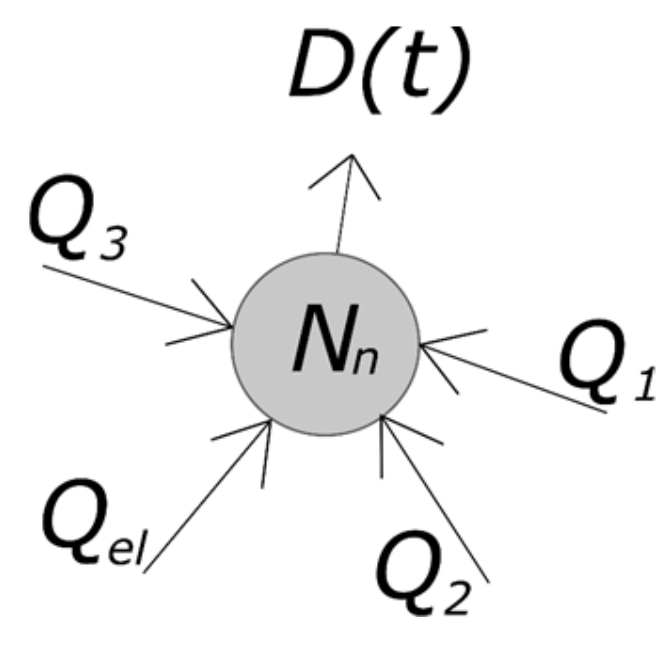
For the end points, the procedure presented in [18] was used, where the continuity law is applied for a generic node, as presented in Figure 1. The flow of a convergent pipe has a positive signal and can be calculated using a positive characteristic line, while a divergent pipe has a negative signal and the negative characteristic line is used. Accordingly, Equation (5) is obtained, which is applied to any node.
Here, and are the numbers of converging and diverging pipes, respectively, connected to the node; and indicate that coefficients correspond to pipes and , respectively; is the hydraulic head on the node; is the flow through a non-pipe element; and are the expressions in brackets in Equation (5); and is the nodal demand at time .
2.2. Database Creation and Proposed Models
To create the database to train the various ANNs, each node of the studied networks was considered as a potential bursting point. Ten values for the leaked flow were simulated, considering that their intensity may range from 5% to 10% of the total inflow of the network. The signal includes information of the initial and final steady-state conditions. A discretization time step of 0.01 s was used. For all the presented methods, the time series used as input corresponded to 60 s and contained information about the entire relevant transient.
For the first model, named LOCP (standing for location method using pressures), the original series of the pressure signals was used as input, resulting in 6000 to 60,000 data points. This method contains very detailed information about the signal and can result in redundancies for the ANN.
The second method, named LOCSAX (standing for location method using SAX), which represents time series though strings, tries to fix this drawback by using symbolic aggregate approximation (SAX) [26] to reduce the amount of information by using a small number of symbols. The representation of time series using symbols has attracted interest in several areas of knowledge, such as computer science, astronomy and medicine, to deal with problems of clustering, classification, indexing and detection of anomalies. Several techniques of symbolic representation of time series for data mining have been proposed in the last decades. Some of them exhibit difficulties derived from the dimensionality of the problems, as they maintain the same dimension of the original data, thus also maintaining the same scale of the problem [26]. SAX is applied in [27] to forecast water demand in WDSs. This technique transforms a time series into a string with reduced data dimensionality, while still providing great ability to compare similarities between time series and to discriminate between them. The pressure time series is divided into a number of segments, and the average value of each segment is classified into one of the letters of an alphabet, as exemplified in Figure 2.
In this work, the number of characters representing the time series varied from 5 to 20, with and being the best combination. Thus, the input for the ANN is a vector containing just characters.
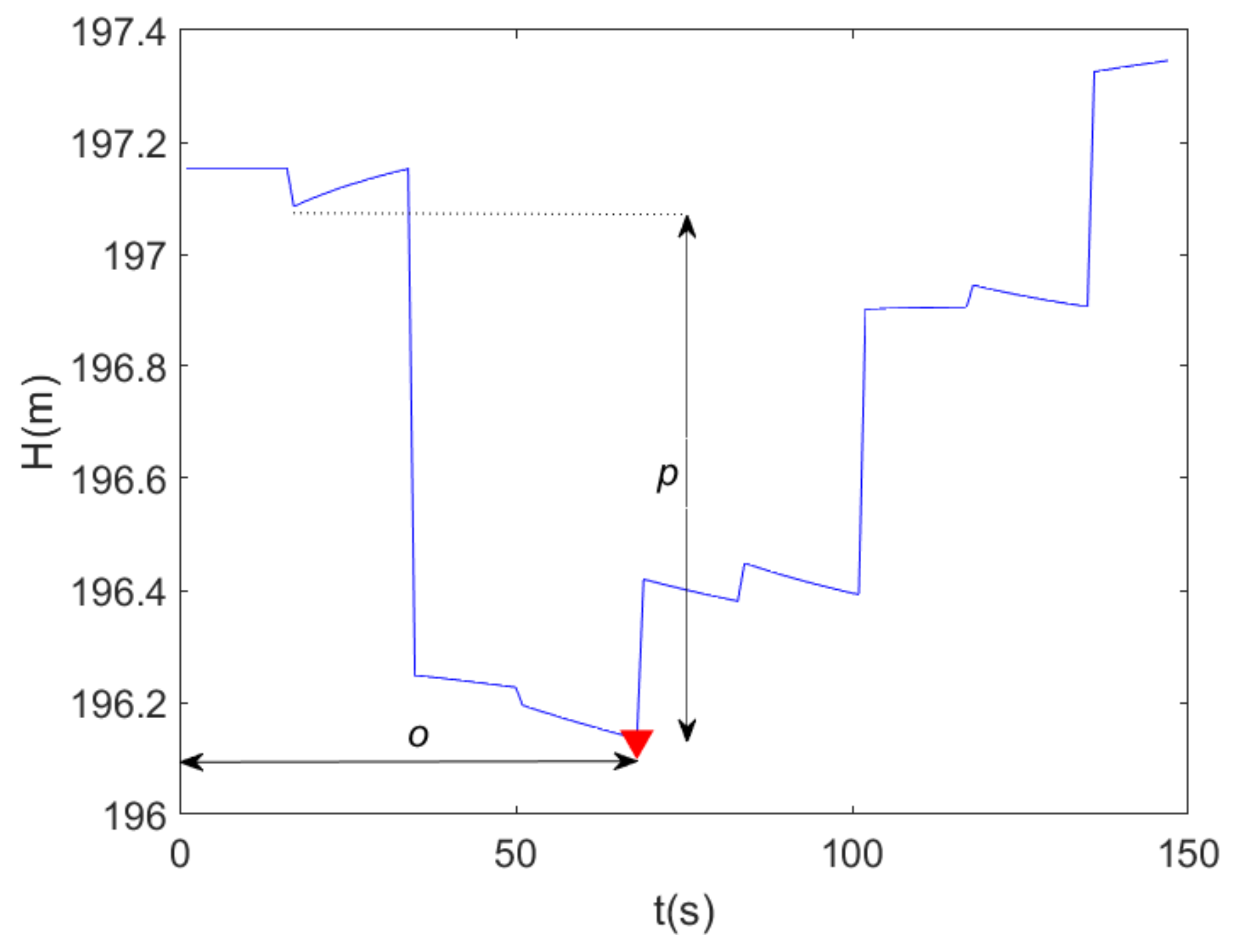
Finally, the third method, named LOCPEAKS (standing for location method using peak pressure information), uses only the most salient information of the transient pressure signal, namely the maximum pressure drop observed () and the time delay for the pressure sensor to record this value (), as illustrated in Figure 3. Although this method contains the essential information about the pressure transient, its limited information can make it difficult for the ANN to distinguish bursts occurring in nodes with similar conditions of flow, elevation and distance to the monitoring points.
In the three methods, the output response of the ANN is the index of the node where the burst occurred and its leaked flow.
2.3. ANN Training for Burst Location
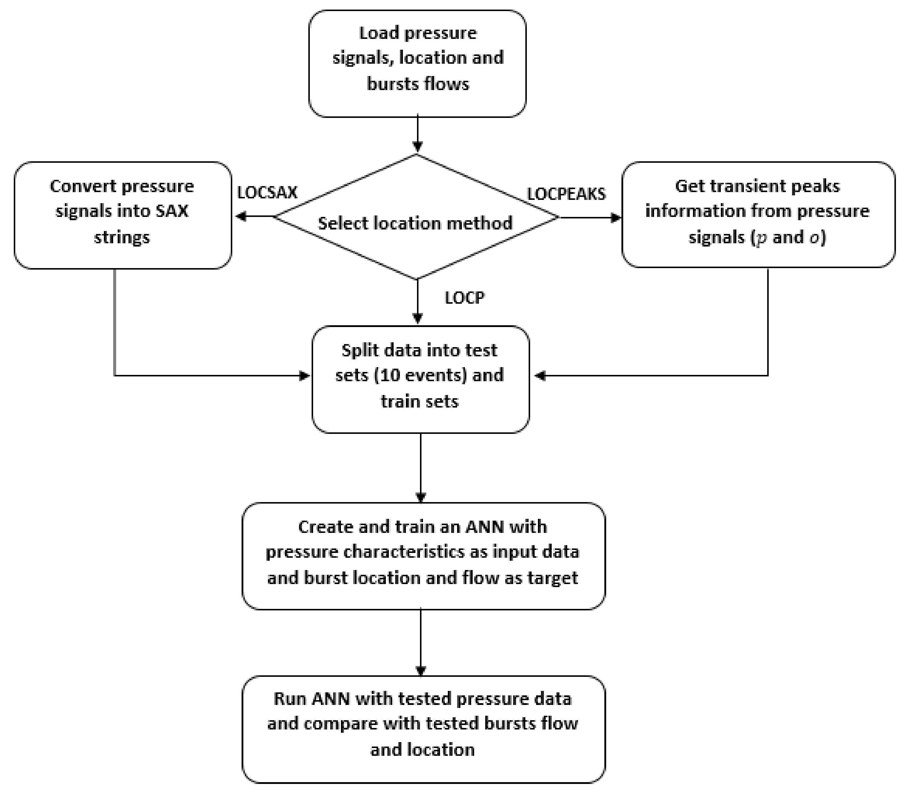
ANNs have been successfully applied in non-linear multivariable function approximations, and as classifiers. The ANN’s ability to predict patterns has found success in practical applications such as WDS calibration and demand forecasting [28,29]. The ANN training process followed the flowchart presented in Figure 4. The database containing the pressure signal together with the location and intensity of the lost flows was loaded and then the representation method was selected. After the preprocessing of the pressure signal according to the selected method, 50% of the database was used for training, 35% for validation, and the remaining 15% was used for testing. The ANN was built with three hidden layers, and with a (20, 40, 20) layer-architecture of neurons. The Levenberg–Marquardt technique was used to obtain the synaptic weights of the neurons, and the stop criteria was set to 500 epochs or a relative change of less than 10−8.
2.4. Clustering Pressure Signal to Improve ANN Efficiency
Each pipe burst creates a unique pressure signal input in each sensor placed in the WDS. Yet, when a pipe burst occurs with different intensity, the shape of the pressure signal is very similar, with just a slight difference in the peaks. In addition, when bursts in two pipes have the same intensity, the respective pressure signals are very similar as well, with some transmission lag. As a result, it is possible to cluster the observed signals, and train specific ANNs for each group, thus reducing the error in the burst location.
To define the clusters, the hybrid methodology proposed by the authors in [30], using SOMs coupled with the k-means algorithm, was used. The neurons obtained using SOMs cluster the input data by their similarity. Calculating the distance between each neuron and the input data, a dissimilarity matrix can be created:
This matrix can be used as input for the k-means algorithm, where various numbers of clusters are considered. Here is the neuron -vector of synaptic weights; and is the input -vector. For this study, the architecture of the SOM was defined following the discussions presented in [30], based on a tradeoff between the quantization error and the training time. The topology followed a hexagonal distribution. The SOM with the best tradeoff had 16 neurons.
Finally, the index [31], shown in Equation (7), was calculated to determine the optimal number of clusters.
In Equation (7), is the number of elements of cluster ; is an element in cluster ; is the centroid of all input data; is the number of clusters; and is the number of input data.
3. Results
3.1. Jardim Laudissi Network
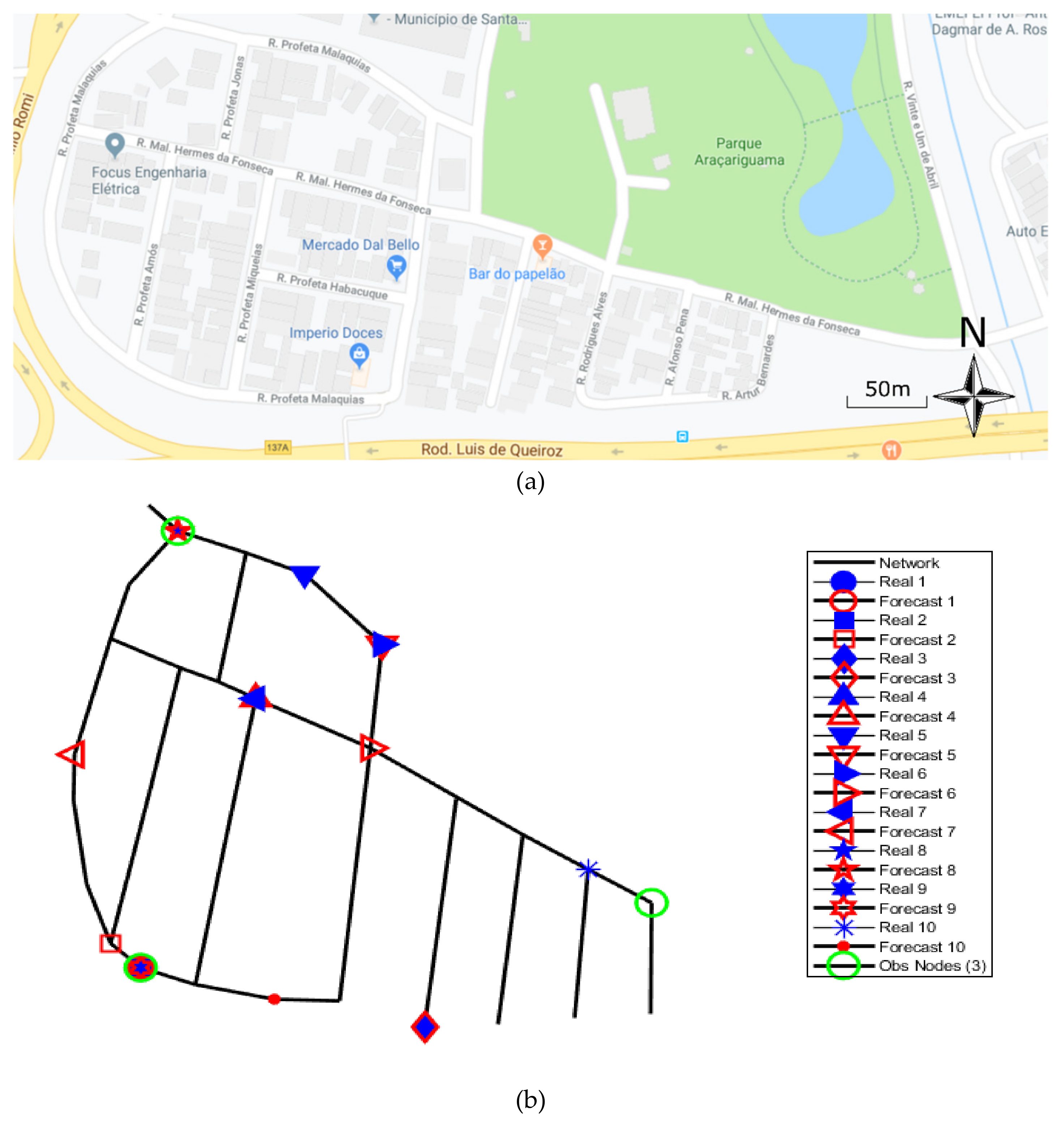
The Jardim Laudissi network is a Brazilian district metered area (DMA) in Piracicaba, São Paulo, having 222 user connections, 2.7 km total pipe length, and three points for pressure monitoring. One monitoring point is at the entrance of the network, and the two others are at critical points in the network (highest and lowest elevations), representing 12% of the 25 nodes of the hydraulic model. Pressure sensors are located to monitor both minimum and maximum pressures inside the DMA and to drive a pressure reduction valve (PRV) installed at the DMA entrance, so as to maintain a suitable pressure control. The network topology and pressure sensor locations (noted as green circles —“Obs nodes (3)”) are presented in Figure 5b. The results of the methods’ application were evaluated both in terms of the Euclidean distance between estimated and real bursting node and the error between estimated and real leaked flow.
The application of LOCP, LOCSAX and LOCPEAKS methods to the Jardim Laudissi network indicated good accuracy in locating events and in assessing their respective flows, as shown in Table 1. The LOCSAX presented the smallest average error for the leaked flow, while the shortest average distance for burst localization was performed by LOCP. Figure 5 shows the results for the LOCP method applied for 10 test scenarios, showing the true burst position and the estimated one.
3.2. Campos do Conde Network
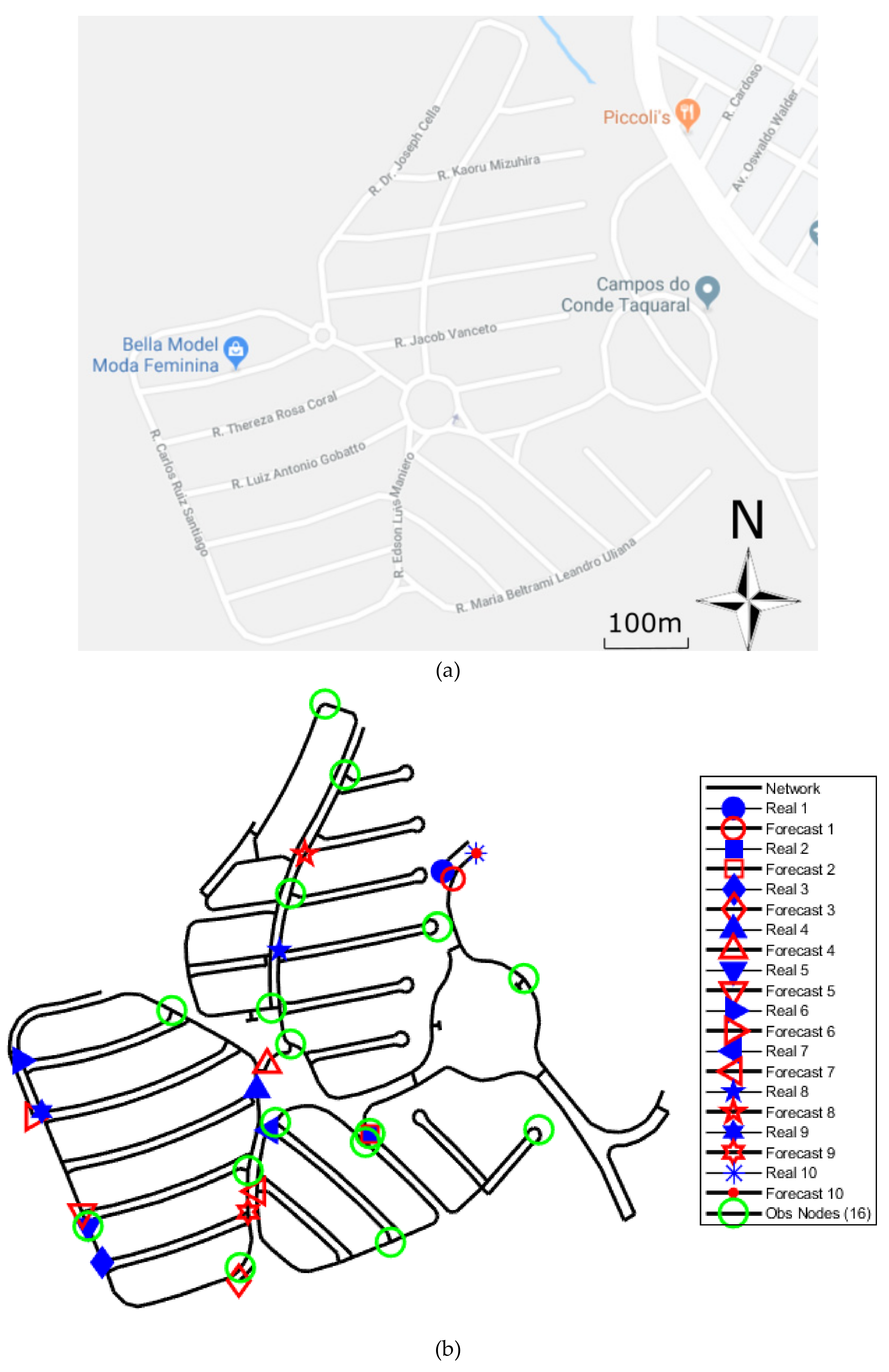
The Campos do Conde network is also a Brazilian DMA with 854 user connections, and has a total network length of approximately 12 km, with diameters varying from 50 to 200 mm. As the Campos do Conde network is a bigger and more complex network, 16 pressure monitoring nodes were considered. This represents 13.5% of the 118 nodes of the hydraulic model of the network, thus following a similar proportion as that used in the previous case. The topology and pressure sensor locations are presented in Figure 6.
The three proposed methods, LCOP, LOCSAX and LOCPEAKs, were applied for this network, and the results are shown in Table 2. In contrast to the Jardim Laudissi network results, here the LOCP method showed the greatest accuracy both for location and forecasting of the leaked flow. Figure 6 shows the results for the LOCP method applied for 10 test scenarios, showing the true burst position and the estimated one.
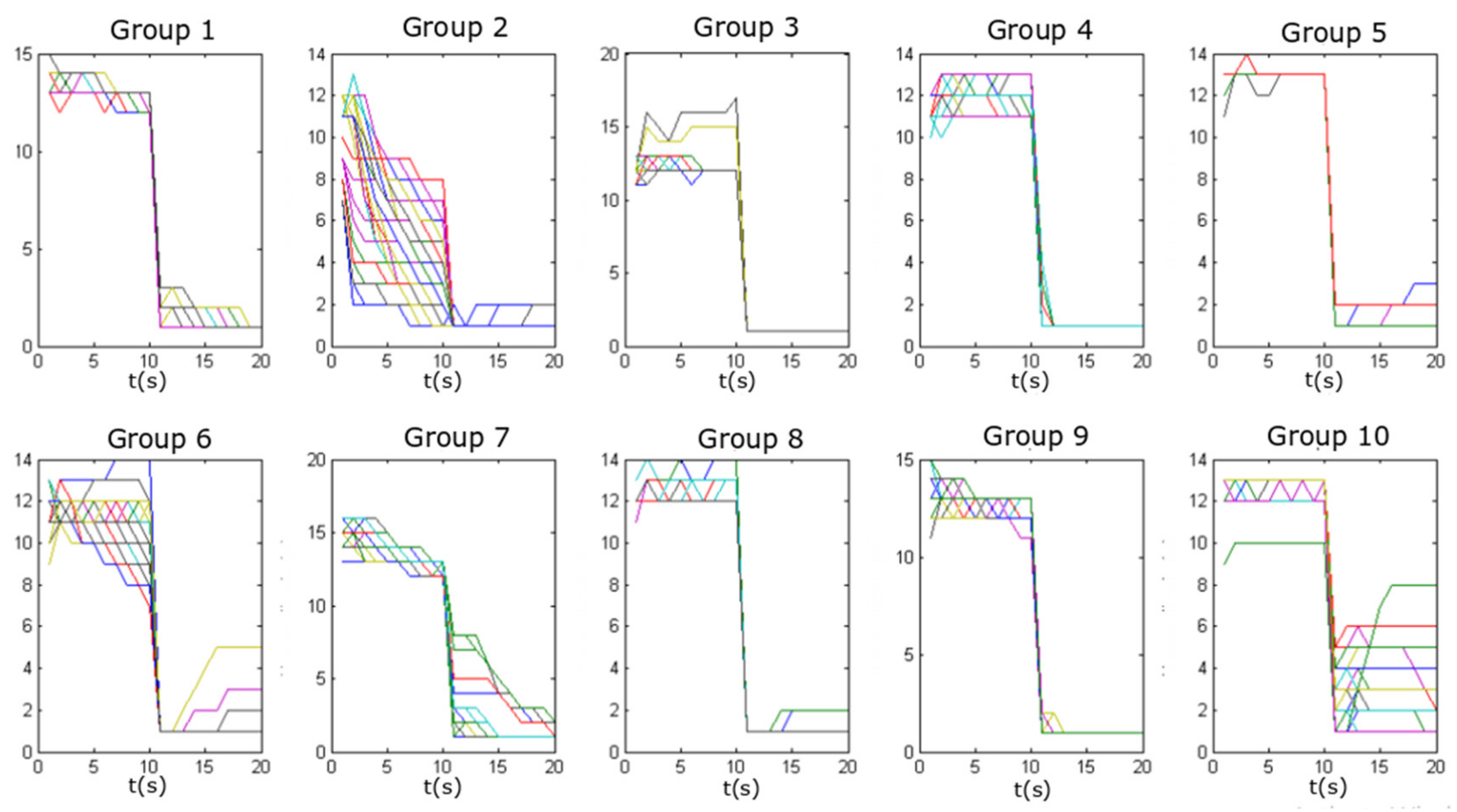
As the database is much larger for Campos do Conde network than it is for the Laudissi network, the above-mentioned clustering procedure using SOMs and k-means was used. As a result, ten groups of transient pressure signals collected by the sensors were created, as shown in Figure 7. In an attempt to simplify the methodology for real networks, the use of a reduced number of sensors was also evaluated. Thus, in addition to the case with sixteen sensors, a midway scenario with eight sensors representing 6.8% of the network nodes and a low-level monitoring scenario with only four sensors representing 3.4% of the network nodes were also studied. The results obtained for the Campos do Conde network are summarized in Table 3. The improvement is clear for all the three methods when the clustering is made, but the LOCP still had the best performance. It is interesting to observe that when using this approach, reducing the number of sensors did not harm the performance when compared with the case with no clustering. In fact, the best performance was observed for the midway (eight sensors) condition, probably due to the reduction of redundant information together with the maintenance of essential sensors for the ANN. Figure 7 presents an instance of the final clustered signals using measurements from eight sensors. It is possible to highlight visible pattern differences between clusters which identify different network regions.
4. Conclusions
The resilience of a WDS strongly depends on good conditions of design, installation and maintenance. However, in operational terms, the reduction of run times of potential bursts allows the reduction of volumes lost in break events which also helps maintain good resilience standards. The pressure signals caused by bursts have an important correlation with their location and magnitude, thus stamping a "hydraulic signature" of these events. For this signature to provide reliable information, the network must be suitably calibrated. Otherwise, the associated uncertainty in pipe characteristics, such as material, age and effective diameter, with well-known great influence on the propagation speed of transient signals, would blur the obtained results, thus turning them useless. In our study we have performed simulations on two networks with perfectly defined characteristics.
In this paper, the use of ANNs as pattern recognizers has succeeded in the identification of hydraulic patterns of various tested bursts. The proposed methods allow the detection and location of bursts in WDSs, after analyzing the characteristics of the transient signals using data acquisition rates compatible with commercial equipment (of the order of 1 kHz), and without the need to measure the inlet flow to the system, which is more difficult to acquire at higher frequencies. The results showed that the LOCP method is the most accurate method to locate bursts. Although the data used to train the ANN are significantly larger for this method, the complete signal appears to contain relevant information that is not well described by the other two methods. Both LOCSAX and LOCPEAKS are able to estimate the burst location with less effort, however these methods are less accurate than LOCP. Even though the use of the complete transient data increases the effort to train the ANNs, this procedure has to be done only once, with the network re-trained sporadically upon the arrival of new data or after modifications in the network topology. Furthermore, the use of clusters to improve the accuracy for burst location estimation reduces the number of data to train the ANNs since thanks to data similarities, the training process is easier. Finally, the clustering of transient signals increased the performance of all three methods and showed that, even in a reduced monitoring scenario, burst location was satisfactory.
In practical terms, this situation contributes to technical and economic feasibility of networks for fast location of breaks, by means of commercially available pressure measurement equipment with very affordable costs compared to flowmeters with the same accuracy. The methods have been tested on two small and medium size networks, which could be seen as district metered areas of larger networks. As a result, we recognize that the application of the proposed methods may be limited by the network size. However, when using transient pressure signals, the effect of a water loss probably will not be detected by a sensor far from the DMA where the burst occurs. This is because of the attenuation process of the pressure wave due to the friction effects. In addition, a larger network is likely to have more pressure sensors available, thus there is more information to process in the ANN training, allowing a broader coverage of the network. As future works, it is recommended to evaluate the methods considering entire large networks using different sampling frequencies for sensors, which will enrich the methodology presented with analyses of the uncertainty derived from pressure sensors in high frequency data acquisition.
Author Contributions
Conceptualization: D.M., B.B., G.M. and E.L.J.; software: D.M. and B.B.; investigation: D.M., B.B., G.M., J.I. and E.L.J.; supervision: B.B., J.I., E.L.J.; writing, review and editing: B.B. and J.I.
Funding
This research received no external funding.
Conflicts of Interest
The authors declare no conflict of interest.
Abbreviations
The following abbreviations are used in this manuscript:
| Abbreviation | Explanation |
| ANN | artificial neural network |
| CH | Caliński-Harabasz (index for cluster quality) |
| DMA | district metered area |
| GA | genetic algorithm |
| LOCP | location method using pressures |
| LOCPEAKS | location method using peak pressure information |
| LOCSAX | location method using SAX |
| MOC | method of characteristics |
| PRV | pressure reduction valve |
| SAX | symbolic aggregate approximation |
| SOM | self-organizing map |
| WDS | water distribution system |
References
- Farley, M.; Trow, S. Losses in Water Distribution Networks; IWA Publishing: London, UK, 2003. [Google Scholar]
- Creaco, E.; Walski, T. Economic Analysis of Pressure Control for Leakage and Pipe Burst Reduction. J. Water Resour. Plan. Manag. 2017, 143, 4017074. [Google Scholar] [CrossRef]
- Campisano, A.; Creaco, E.; Modica, C. RTC of valves for leakage reduction in water supply networks. J. Water Resour. Plan. Manag. 2009, 136, 138–141. [Google Scholar] [CrossRef]
- Campisano, A.; Modica, C.; Reitano, S.; Ugarelli, R.; Bagherian, S. Field-Oriented Methodology for Real-Time Pressure Control to Reduce Leakage in Water Distribution Networks. J. Water Resour. Plan. Manag. 2016, 142, 04016057. [Google Scholar] [CrossRef]
- Vítkovský, J.P.; Simpson, A.R.; Lambert, M.F. Leak Detection and Calibration Using Transients and Genetic Algorithms. J. Water Resour. Plan. Manag. 2000, 126, 262–265. [Google Scholar] [CrossRef]
- Pérez, R.; Puig, V.; Pascual, J.; Quevedo, J.; Landeros, E.; Peralta, A. Methodology for leakage isolation using pressure sensitivity analysis in water distribution networks. Control Eng. Pract. 2011, 19, 1157–1167. [Google Scholar] [CrossRef] [Green Version]
- Jung, D.; Kim, J.H. Robust Meter Network for Water Distribution Pipe Burst Detection. Water 2017, 9, 820. [Google Scholar] [CrossRef]
- Covas, D.; Ramos, H. Hydraulic transients used for leakage detection in water distribution systems. In Proceedings of the 4th International Conference in Water Pipeline Systems, York, UK, 28–30 March 2001. [Google Scholar]
- Colombo, A.F.; Lee, P.; Karney, B.W. A selective literature review of transient-based leak detection methods. HydroResearch 2009, 2, 212–227. [Google Scholar] [CrossRef]
- Choi, D.Y.; Kim, S.-W.; Choi, M.-A.; Geem, Z.W. Adaptive Kalman Filter Based on Adjustable Sampling Interval in Burst Detection for Water Distribution System. Water 2016, 8, 142. [Google Scholar] [CrossRef]
- Christodoulou, S.E.; Kourti, E.; Agathokleous, A. Waterloss detection in water distribution networks using wavelet change-point detection. Water Resour. Manag. 2017, 31, 979–994. [Google Scholar] [CrossRef]
- Misiunas, D. Failure Monitoring and Asset Condition Assessment in Water Supply Systems. Ph.D. Thesis, Vilniaus Gedimino Technikos Universitetas, Vilnius, Lithuania, 2008. [Google Scholar]
- Guo, X.; Yang, K.; Guo, Y. Leak detection in pipelines by exclusively frequency domain method. Sci. China Ser. E Technol. Sci. 2012, 55, 743–752. [Google Scholar] [CrossRef]
- Holloway, M.B.; Chaudhry, M.H. Stability and accuracy of waterhammer analysis. Adv. Water Resour. 1985, 8, 121–128. [Google Scholar] [CrossRef]
- Sanz, G.; Pérez, R.; Kapelan, Z.; Savic, D. Leak detection and localization through demand components calibration. J. Water Resour. Plan. Manag. 2015, 142, 04015057. [Google Scholar] [CrossRef]
- Zhang, Q.; Wu, Z.Y.; Zhao, M.; Qi, J.; Huang, Y.; Zhao, H. Leakage Zone Identification in Large-Scale Water Distribution Systems Using Multiclass Support Vector Machines. J. Water Resour. Plan. Manag. 2016, 142, 04016042. [Google Scholar] [CrossRef]
- Mounce, S.R.; Machell, J. Burst detection using hydraulic data from water distribution systems with artificial neural networks. Urban Water J. 2006, 3, 21–31. [Google Scholar] [CrossRef]
- Almeida, A.B.; Koelle, E. Fluid Transients in Pipe Networks; Computational Mechanics Publications: Southampton, UK, 1992. [Google Scholar]
- Covas, D.I.C.; Ramos, H.M.; De Almeida, A.B. Standing Wave Difference Method for Leak Detection in Pipeline Systems. J. Hydraul. Eng. 2005, 131, 1106–1116. [Google Scholar] [CrossRef]
- Srirangarajan, S.; Allen, M.; Preis, A.; Iqbal, M.; Lim, H.B.; Whittle, A.J. Wavelet-based burst event detection and localization in water distribution systems. J. Signal Process. Syst. 2013, 72, 1–16. [Google Scholar] [CrossRef]
- Liggett, J.A.; Chen, L. Inverse Transient Analysis in Pipe Networks. J. Hydraul. Eng. 1994, 120, 934–955. [Google Scholar] [CrossRef]
- Caputo, A.C.; Pelagagge, P.M. An inverse approach for piping networks monitoring. J. Loss Prev. Process. Ind. 2002, 15, 497–505. [Google Scholar] [CrossRef]
- Van Zyl, J.E. Theoretical modeling of pressure and leakage in water distribution systems. Procedia Eng. 2014, 89, 273–277. [Google Scholar] [CrossRef]
- Wylie, E.B.; Streeter, V.L.; Suo, L. Fluid Transients in Systems; Prentice Hall: Englewood Cliffs, NJ, USA, 1993; Volume 1, p. 464. [Google Scholar]
- Izquierdo, J.; Iglesias, P. Mathematical modelling of hydraulic transients in complex systems. Math. Comput. Model. 2004, 39, 529–540. [Google Scholar] [CrossRef]
- Lin, J.; Keogh, E.; Wei, L.; Lonardi, S. Experiencing SAX: A novel symbolic representation of time series. Data Min. Knowl. Discov. 2007, 15, 107–144. [Google Scholar] [CrossRef]
- Navarrete-López, C.; Herrera, M.; Brentan, B.M.; Luvizotto, E.; Izquierdo, J. Enhanced Water Demand Analysis via Symbolic Approximation within an Epidemiology-Based Forecasting Framework. Water 2019, 11, 246. [Google Scholar] [CrossRef]
- Meirelles, G.; Manzi, D.; Brentan, B.; Goulart, T.; Luvizotto, E. Calibration Model for Water Distribution Network Using Pressures Estimated by Artificial Neural Networks. Water Resour. Manag. 2017, 31, 4339–4351. [Google Scholar] [CrossRef]
- Adamowski, J.; Chan, H.F. A wavelet neural network conjunction model for groundwater level forecasting. J. Hydrol. 2011, 407, 28–40. [Google Scholar] [CrossRef]
- Brentan, B.; Meirelles, G.; Luvizotto, E., Jr.; Izquierdo, J. Hybrid SOM+ k-Means clustering to improve planning, operation and management in water distribution systems. Environ. Model. Softw. 2018, 106, 77–88. [Google Scholar] [CrossRef]
- Caliński, T.; Harabasz, J. A dendrite method for cluster analysis. Commun. Stat. Theory Methods 1974, 3, 1–2. [Google Scholar] [CrossRef]
Figure 1.
Generic node of a water distribution system (WDS).

Figure 2.
Converting a time series (blue line) to symbolic aggregate approximation (SAX) code using an alphabet of three letters: (a) original time series () and discretization () for ; (b) string (baabccbc) conversion of , using an alphabet of symbols (source: adapted from [27]).
Figure 2.
Converting a time series (blue line) to symbolic aggregate approximation (SAX) code using an alphabet of three letters: (a) original time series () and discretization () for ; (b) string (baabccbc) conversion of , using an alphabet of symbols (source: adapted from [27]).

Figure 3.
Pressure drop amplitude () and its time delay during a pipe burst () at certain sensor (red triangle). Axes are in seconds and water column meters for total head.
Figure 3.
Pressure drop amplitude () and its time delay during a pipe burst () at certain sensor (red triangle). Axes are in seconds and water column meters for total head.

Figure 4.
Flowchart of artificial neural network (ANN) training for burst location.

Figure 5.
(a) Scale map of the district metered area (DMA) Laudissi: adapted from Google Maps (b) Results for test scenarios using LOCP method in Jardim Laudissi network.
Figure 5.
(a) Scale map of the district metered area (DMA) Laudissi: adapted from Google Maps (b) Results for test scenarios using LOCP method in Jardim Laudissi network.

Figure 6.
(a) Scaled map of the DMA Campos do Conde: adapted from Google Maps (b) Results for test scenarios using LOCP method in Campos do Conde network.
Figure 6.
(a) Scaled map of the DMA Campos do Conde: adapted from Google Maps (b) Results for test scenarios using LOCP method in Campos do Conde network.

Figure 7.
Clustering for the LOCP method using eight sensors in the Campos do Conde network.


Table 1.
Jardim Laudissi network results for distance and leaked flow.
| Method | LOCP | LOCSAX | LOCPEAKS |
|---|---|---|---|
| Average error in burst flow forecasting (%) | 25 | 1 | 4 |
| Average error in burst location (m) | 55 | 80 | 83 |
Table 2.
Campos do Conde results for leaked flow and distance.
| Method | LOCP | LOCSAX | LOCPEAKS |
|---|---|---|---|
| Average error in burst flow forecasting (%) | 2 | 16 | 9 |
| Average error in burst location (m) | 82 | 109 | 280 |
Table 3.
Campos do Conde results with clustering.
| Number of Sensors | Method | Average Error in Burst Location (m) |
|---|---|---|
| 16 | LOCP | 67 |
| LOCSAX | 89 | |
| LOCPEAKS | 156 | |
| 8 | LOCP | 52 |
| LOCSAX | 156 | |
| LOCPEAKS | 171 | |
| 4 | LOCP | 73 |
| LOCSAX | 133 | |
| LOCPEAKS | 172 |
© 2019 by the authors. Licensee MDPI, Basel, Switzerland. This article is an open access article distributed under the terms and conditions of the Creative Commons Attribution (CC BY) license (http://creativecommons.org/licenses/by/4.0/).
Share and Cite
MDPI and ACS Style
Manzi, D.; Brentan, B.; Meirelles, G.; Izquierdo, J.; Luvizotto, E., Jr. Pattern Recognition and Clustering of Transient Pressure Signals for Burst Location. Water 2019, 11, 2279. https://doi.org/10.3390/w11112279
AMA Style
Manzi D, Brentan B, Meirelles G, Izquierdo J, Luvizotto E Jr. Pattern Recognition and Clustering of Transient Pressure Signals for Burst Location. Water. 2019; 11(11):2279. https://doi.org/10.3390/w11112279
Chicago/Turabian StyleManzi, Daniel, Bruno Brentan, Gustavo Meirelles, Joaquín Izquierdo, and Edevar Luvizotto, Jr. 2019. "Pattern Recognition and Clustering of Transient Pressure Signals for Burst Location" Water 11, no. 11: 2279. https://doi.org/10.3390/w11112279
Note that from the first issue of 2016, this journal uses article numbers instead of page numbers. See further details here.