An Empirical Research on Influence Factors of Industrial Water Use


1
College of Hydrology and Water Resources, Hohai University, No. 1, Xikang Road, Nanjing 210098, China
2
State Key Laboratory of Hydrology-Water Resources and Hydraulic Engineering, Nanjing Hydraulic Research Institute, Nanjing 210029, China
3
Research Center for Climate Change, Ministry of Water Resources, Nanjing 210029, China
*
Author to whom correspondence should be addressed.
Water 2019, 11(11), 2267; https://doi.org/10.3390/w11112267
Submission received: 1 September 2019
/
Revised: 12 October 2019
/
Accepted: 23 October 2019
/
Published: 29 October 2019
(This article belongs to the Special Issue Water Resources, Socio-Economic Development and the Environment)
Abstract
:The contradiction between increasing demand and current supply has affected the healthy development of industry. Investigating the key influence factors of industrial water use change has important practical significance for water resource management. In this study, the authors propose the vector autoregression model to analyze the dynamic influences of industrial development, technological progress, and environmental protection on industrial water use change, and take Jiangsu Province, China as a case study. Results show that each of the factors had different effects during 2001–2015, in which industrial development was the greatest contributor to the change of industrial water use and showed a positive effect in the forecast period; technological progress played a major role in reducing industrial water use, but the negative effect weakened periodically over time; environmental protection also had a positive influence in the early forecast period, and then showed a marginal effect with time. Results of this study could assist the relevant authorities to formulate appropriate industrial development planning and water saving policies, and to reasonably control the industrial water demand.
1. Introduction
Water plays a crucial role in different production processes. According to its function and purpose, industrial water use can be classified as production water use, cooling and thermal water use, and miscellaneous water use [1,2]. Compared to agriculture and domestic water use, water for industrial use is more complex, and it is more easily affected by changes in the external environment such as industrial development, production level upgrading, environmental protection requirements, and climate change [3,4,5,6,7].
With the rapid progress of industrialization and urbanization, water shortage has become the bottleneck restricting sustainable industrial development in China, especially for the water-intensive industry [8,9]. In addition, over the recent decades, multi-purpose water management has reflected the different functions provided by rivers, which can be complementary or conflicting [10]. This calls for more integrated water resource management. The implementation of various effective measures of integrated water resource management, to alleviate the constraints of water shortages on economic and social development, can be categorized as structural measures (water conservancy projects, such as building dams and water transfers) and non-structural measures (water resource management, such as formulating water saving regulation). Due to financial and environmental restrictions, a water shortage crisis is more likely to be solved through water resource management strategy than by building water conservancy projects [11]. The Chinese government has set up “three red lines” to promote economic and social development and adapt to water resource carrying capacity, which put forward clear requirements and targets for the amount of water withdrawal, water usage efficiency, and quantity of pollution discharge; preliminary results have been achieved [12]. In view of the process and characteristics of water utilization, the purposes of water resource management for industry are to decrease fresh water withdrawal and effluent discharge, and to improve the utilization rate of water resources.
Steady growth of economic development continues to drive water demand for industry [8,13]; it is projected that water withdrawal and water consumption will both show an increasing trend in the future, and that the industrial water demand of China in the 2050s will be twice that of the 2010s under a sustainability scenario [6,14]. In addition, the decrease of water resources availability and increased use of cooling water caused by climate change exacerbate the degree of water resource constraints on industrial development [7,15,16]. Researchers have begun to pay more attention to water network optimization based on substance flow analysis and pinch analysis under multiple objectives and scales to achieve efficient utilization of water resources [17,18,19]. Additionally, integrated water management strategies covering different segments have been proposed, which include water monitoring, water system optimization, and wastewater reuse, to assess water conservation potential [2]. From the macro level, there are relatively few studies on the influence of external environmental factors on the change of industrial water use. Moreover, the existing studies have emphasized the analysis of the impacts of economic development and technical innovation on water use [20,21]. Usually, the influence factors of industrial water use are complex, including industrial development, water-saving technologies, environmental protection, and climate change [22,23]. In particular, industrial production is accompanied by wastewater and exhaust emissions. Under strict requirements of ecological and environmental protection in China, the high standards regulating discharge of industrial wastewater and emission of industrial waste gas have been set up and implemented, with higher requirements being put on the manufacturing sector. Discharge of industrial wastewater and exhaust gas up to the allowed standard have an impact on industrial water demand [24]. Thus, environmental protection should be included among the main influence factors for further analysis regarding their impact on the change of industrial water use.
Various methods have been applied to quantify the promotion or inhibition effects of various factors on water use. The representative models include the Structural Decomposition Analysis (SDA) method, STIRPAT model, Laspeyres method, Input–output method, and Logarithmic Mean Divisia Index (LMDI) method [25,26]. Applying the factor decomposition model, Sun and Wang [27] measured the economic growth effect, industrial structure effect, water intensity effect, and mixing effect of the driving force of water utilization change. Cazcarro et al. [28] explored the impacts of technology, the input substitution process, and the changes in final demand on water consumption for the years 1980–2007 using the input–output model. Yang et al. [29] adopted the dynamic SDA method to investigate the influence of socioeconomic determinants on water footprint evolution. Shang et al. [30] decomposed the driving forces of industrial water use by the LMDI and the refined Laspeyres models. The above-mentioned quantitative analysis methods have static problems and cannot reflect the dynamic relationship between influencing factors and water use. In fact, the change of industrial water use is a dynamic process. The vector autoregression (VAR) model, as a simultaneous equation model, can not only reveal the interdependencies among variables, but can also forecast the dynamic relationship between variables. As it is easy to understand and operate, it has been adopted for analysis in various fields, especially in the economic and environmental fields [31,32,33,34,35]. Nevertheless, there is still a lack of studies that adopt the VAR model to investigate the relationship between influence factors and industrial water use.
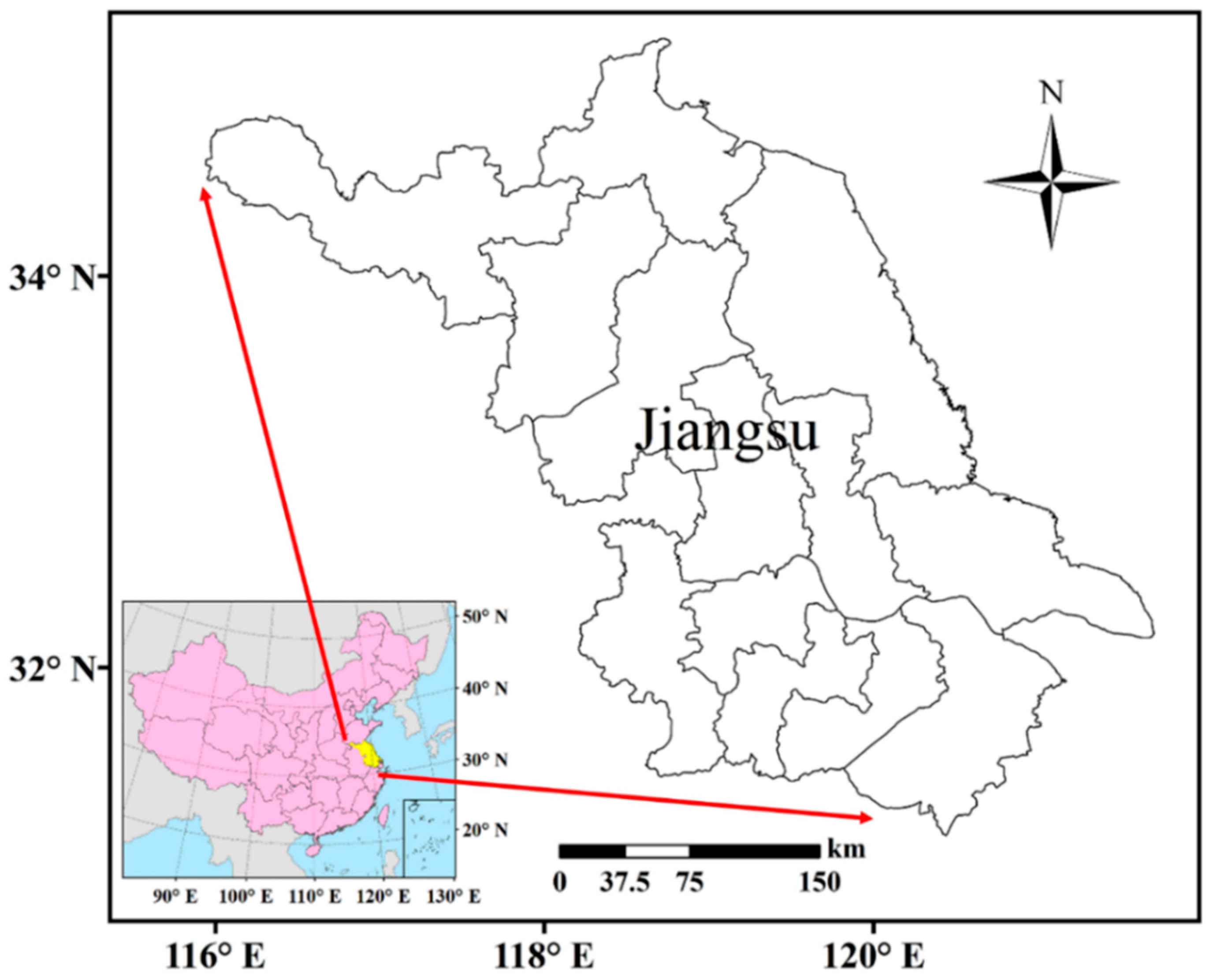
This paper has three aspects of innovation and contribution that differ from previous studies. Firstly, we introduce environmental protection, which has a close connection with industrial water use, as an influence factor to analyze the impact on industrial water use. Previous studies seldom considered this factor. Secondly, compared to static analysis of previous studies, the VAR model was employed to reveal the dynamic relationship between selected influence factors and industrial water use. This could give more comprehensive information for policy makers. Thirdly, the majority of existing studies emphasized the analysis of the influence of water use change on a regional scale. We focus on the impact analysis of changes in sectoral water use within the region; Jiangsu Province is selected as the study area, which is the largest industrial province of China and faces environmental protection problems. This is an ideal representative to carry out the analysis of industrial water use change. The location of Jiangsu Province is shown in Figure 1.
2. Materials and Methods
2.1. Data
All data reflect the actual situation of Jiangsu Province from 2001 to 2015. The annual amount of industrial water use () and water use per unit of industrial output () were acquired from Jiangsu Water Resources Bulletin. Data of industrial output () were obtained from Jiangsu Statistical Yearbook. In order to eliminate the effect of rising prices and inflation, industrial output was calculated at constant prices (Year 2000 = 100). The annual discharge (emission) of industrial wastewater, sulfur dioxide, and dust were extracted from China Environmental Statistics Yearbook and Jiangsu Statistical Yearbook. The statistical summary of all variables in this research is shown in Table 1.
2.2. VAR Model
The VAR model is widely used for time series analysis, which was first proposed by Sims [36]. The model constructed by the function described by each endogenous variable is the lag value of all endogenous variables in the system. Additionally, the model, without any prior constraints, is based on time series data to determine dynamic relationship of endogenous variables instead of theory. Thus, the VAR model is applied to analyze the dynamic connection between industrial water use and its influencing factors.
The model consists of multiple simultaneous equations, where the endogenous variable is located on the left of the equation, and the right is its own hysteresis and the lag of other endogenous variables. The general simplified form of the VAR (p) model with lag order p can be expressed as:
where is a endogenous variable vector, p is lag order, u is a vector of constant terms, are parameter matrices, and represents a random error column vector.
The dynamic nexus between industrial water use () and industrial development (), technological progress (), and environmental protection () needs to be explored, and the four variables mentioned above were selected to construct the VAR system. The industrial output was used to reflect the industrial development variable. The water use per unit of industrial output was selected to represent technological progress. The discharge or emission intensity of industrial wastewater discharge, sulfur dioxide emissions, and dust emissions was used to comprehensively reflect the environmental protection variable. However, three environmental protection variables may cause the analysis of the relationship between environmental protection and industrial water use change to be more complex. In order to solve this problem, the integrated index method was adopted for conversion of multiple variables of environment protection into an environmental regulation strength (ERS) indicator, and the ERS indicator was used to reflect environmental protection, which is expressed by . The specific process of the comprehensive index method follows that of Fu and Li [37]. The definitions of all variables are shown in Table 2.
Table 1 and Table 2 show that the dimensions of the four variables are different and there are orders of magnitude differences. Logarithmic treatment is an effective method which could avoid the sharp fluctuation of data and eliminate the possible heteroscedasticity, and not change the characteristics of the time series data [38]. It has been commonly used in VAR model variable time series stationarity testing in previous studies [31,39]. Therefore, natural logarithm treatment was performed on the original data sets, and the data sets are expressed as , , , and , where , , , and refer the industrial water use, industrial development, technological progress and environmental protection, respectively.
As mentioned above, the VAR system consists of the following four variables: Industrial water use (Wt), industrial development (Gt), technological progress (It), and environmental protection (Et). According to Equation (1), the specific form of VAR (p) is as follows:
It should be noted that Equation (2) is the embodiment of the specific form of the original model, and no modifications have been made to the original model.
Testing the stationarity of the time series of each variable is the premise of applying the VAR model, which could avoid the phenomenon of pseudo-regression caused by the instability of variables. Thus, a stationarity test should be performed on the time series before build the model. Many methods have been developed for the stationarity test, and unit root test is the most commonly used method [40]. Three common unit root test methods were applied: The Augmented Dickey–Fuller test (ADF) test, the Kwiatkowski Phillips Schmidt Shin (KPSS) test, and the Phillips Perron (PP) test [41,42,43]. The ADF test is a widely considered and chosen method. However, in small samples, it has its own insurmountable defects, and the validity of the test results is affected [44]. The PP test was selected to supplement the ADF test. The principle of the KPSS test is different from the above two methods, having the null hypothesis that the time series is stationary rather than having a unit root as hypothesized by the ADF test and PP test. It can make up for the defects of ADF and PP test methods [42,45]. These three methods are complementary to each other in verifying the unit root test process, which makes the test result more comprehensive and persuasive.
In practical application, a key issue is the optimal lag order selection. Generally, the selection principle of lag order tends to choose a larger value to take full advantage of variable information of the constructed model. However, the greater the lag order, the more parameters need to be estimated, and degrees of freedom of the model are reduced correspondingly [46]. Therefore, balancing lag order selection and degrees of freedom of the model needs to be taken into consideration.
3. Results
3.1. Variable Description
According to the annual data of the variables, we depict the trends of industrial water use, industrial output, water use per unit of industrial output, and environmental regulation strength. As shown in Figure 2, industrial water use increased rapidly from 2001 to 2007, then showed a declining trend, especially after 2012. This is mainly due to the establishment of water-saving society and implementation of the strictest water resources management system. Industrial output showed a significant upward trend with an average annual growth rate of 13.0%. Water use per unit of industrial output reflected a gradual decreasing trend, which suggests that industrial water use efficiency has been gradually improved. Environmental regulation strength generally presented a fluctuating downward trend, which indicates that environmental protection has achieved remarkable results, and that the wastewater and waste gas emissions have been effectively controlled.
3.2. The Unit Root Test Analysis
ADF, KPSS, and PP methods were selected to verify the stationarity of time series of variables. The results of unit root test of each variable are shown in Table 3.
The ADF test and PP test suggest that time series of , , and are integrated of order one (I(1)), whereas the first-order differences of the time series are integrated of order zero (I(0)), which confirms the hypothesis that the time series of , , and have a unit root. The KPSS test shows different results compared to the ADF and PP tests, because the null hypothesis is the opposite of the other two methods, so it also shows that the time series of , and have a unit root. For the variable , the ADF and PP tests suggest stationarity; the KPSS test shows that it is not stationary. The industrial output, which expressed in terms of , is a macroeconomic index. Generally speaking, macroeconomic data will be stable after first-order difference. Therefore, through comprehensive analysis of the test results and based on previous research [47], we deem the time series of the four variables are all I (1).
As mentioned above, the four variables are all integrated of order one, meaning that the model might be unstable and the impulse response function might be not convergent if the VAR model is established directly, therefore, the VAR model was established by first order difference of each variable, and it is also agreed that the difference of variables is still expressed by the names of , , , and without affecting the understanding of the following contents.
3.3. The Optimal Lag Order Analysis
It is particularly important to choose the lag order while building a VAR model. The selected optimal lag order could maximize the fitness of the forecast process with statistical time series and minimize the measure of forecast precision. The most common procedure for VAR order selection is application of model selection criteria. In this paper, the sequential modified LR test statistic (LR), Final prediction error (FPE), Akaike information criterion (AIC), Schwarz information criterion (SC), and Hannan–Quinn information criterion (HQ) criteria are exploited to jointly determine the optimal order. As shown in Table 4, the results are all in agreement that p = 1 is the optimal lag order.
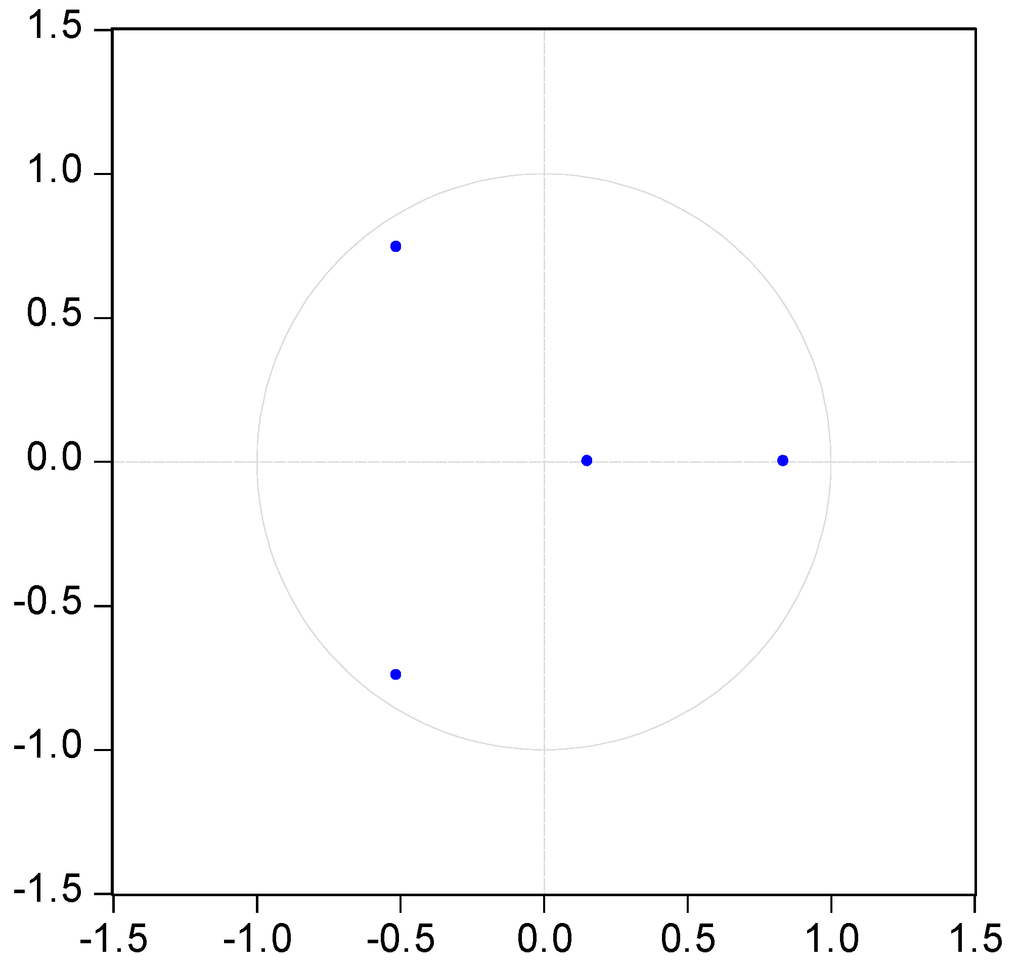
3.4. Model Stability Test
The stability of the model directly affects the validity of the variance decomposition and impulse response analysis results. Therefore, the stability test must be formulated to verify whether the model is stable or not. The necessary and sufficient condition for the stability of the VAR model is that all the eigenvalues of the model characteristic equation are outside the unit circle, that is to say, the inverse eigenvalues of the model characteristic equation are within the unit circle [38]. The results are reflected in Figure 3, and it serves to show that all the inverse eigenvalues of the model’s characteristic equation are within the unit circle, which indicates that the built VAR model is stable.
3.5. Variance Decomposition Analysis
Variance decomposition analysis is normally a method that explores the relative effects of variables [48]. It is used to analyze the contribution degree measured by forecast variance of a specific shock to the endogenous variables of model and gives the relative importance information of each structural shock that affects the variable in the VAR model. Hence, it is able to clearly tell us the proportion of forecast variance produced by all variables with specific shocks on a specified variable at a specified time horizon [31,39].
Table 5 describes the percentage of forecast error variance of the shocked by all variables for the ten-year period. For the industrial water use change, in addition to its own influence, industrial output shock accounts for the largest proportion of the change of industrial water use. It has an increasing effect on industrial water use change with time, from around 15.3% in the first period, increasing to 24.1% in the end, and shows a fluctuating upward trend, which indicates that industrial water use and industrial development have a strong positive correlation. The environmental protection shock ranks second to industrial development. The contribution of environmental protection has increased from 14.2% in the first period to 14.8% in the second period, then downward to the minimum 13.2%, and maintains an upward trend until the end period. The influence of technological progress on industrial water use is basically consistent with the trend of environmental protection, but the contribution degree is slightly lower than that of environmental protection. In summary, industrial development, technological progress, and environmental protection have increasing effects on industrial water use at a specified time period, however, the influence trend does not increase linearly, but fluctuates.
3.6. Impulse Response Analysis
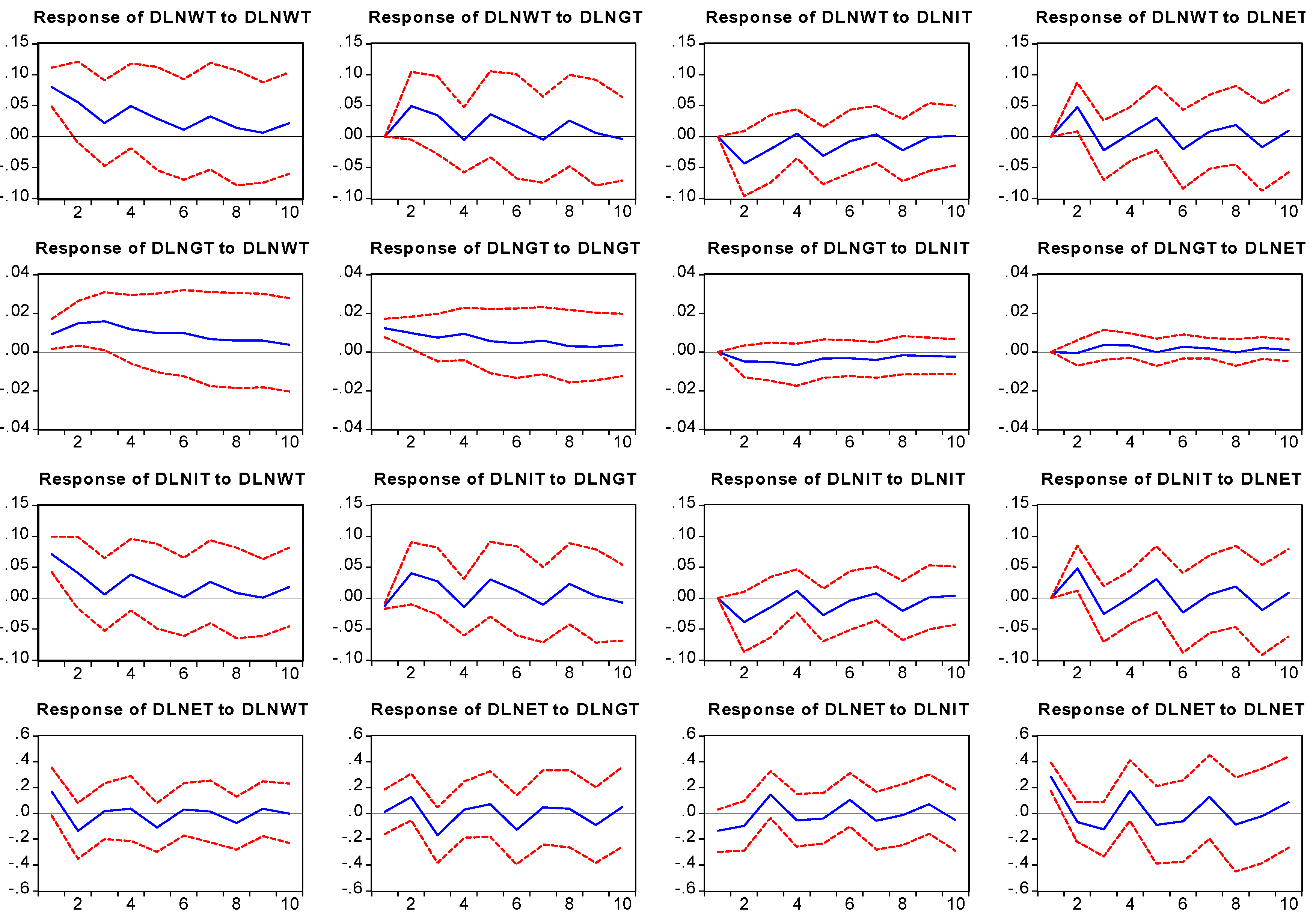
The impulse response functions (IRFs) were applied to analyze the dynamic response of the system. Particularly, they describe the dynamic response of applying a standard deviation on the random error term on all endogenous variables [48]. This method not only reflects the dynamic relationship between different variables, but also identifies the impact of all endogenous variables with a shock in the model at a specified time horizon and quantify the influence degree of the shock.
The IRFs were generated as shown in Figure 4. One standard deviation shock to industrial development () promotes industrial water use directly for 2 years, reaches the maximum positive response at the second period, and then exhibits periodic fluctuation change with time. It reflects nearly a positive response within the whole specified time period, which implies that industrial development will continue to promote industrial water use over the forecast period, but the positive effect will decrease over time. As China’s largest industrial province, the industrial output of Jiangsu Province has increased considerably, at the average annual growth rate of 13.4% from 2001 to 2015 [49]. The corresponding industrial water use showed an increasing trend from 2001 to 2013. Although industrial development promotes the demand for industrial water, the promotion will not be always sustainable. With the promotion and strength of water resource management, industrial water-saving technology has been popularized and applied, and the growth trend of industrial water use has been effectively curbed. Industrial water use dropped significantly after 2013, which was a response to the implementation of the most stringent water resource management system. With orderly progress of industrialization and urbanization, the scale and output of Jiangsu Province industries in the future will be expected to maintain steady and sustained growth, and the demand for industrial water will increase further. Although integrated water resource management, which includes water-saving technology application, water resource management system implementation, and so on, could restrain the industrial water demand, technological progress has limited impact on reducing water use with time, and industrial development will still play the dominant role in promoting the industrial water demand [50]. Thus, adapting to the carrying capacity of water resources is a prerequisite for future industrial development [51].
The industrial water use indicates a significant negative response to technological progress (), which means that technological progress could inhibit industrial water use. As shown in Figure 4, the negative effect of technological progress on industrial water use reached its maximum in the second period and decreased periodically with time. Correspondingly, water use per unit of industrial output in Jiangsu Province dropped obviously from 333.64 m3/t in 2001 to 49.97 m3/t in 2015. Meanwhile, the recycling ratio of industrial water utilization in Jiangsu Province increased from 57% in 2005 to about 70% in 2015 [49] as the improvement of industrial water utilization level and efficiency reduced the demand for fresh water. Nevertheless, water use per unit of industrial output decreased slowly and showed a steady trend from 2013 to 2015. That indicates that technological progress could not maintain a state of rapid innovation, as it has a certain periodicity, and that the water-saving effect of technological progress will be weakened with the passage of time and the increase of industrial scale, correspondingly [7]. Coupled with Jiangsu’s continued industrial growth, the restraining effect of technological progress on industrial water demand is limited, which explains the failure of technological progress to sustain a significant negative effect over the whole forecast period, and presents a periodic decay trend. Besides, the response of technological progress to one standard deviation shock in industrial water use is positive over the forecast period, which implies the increasing of industrial water use will promote technological progress.
The industrial water use shows a positive response to environmental protection () at the early time period, reaches its maximum in the second period, and then fluctuates near zero from the third period to the end period. This indicates that the strengthening of environmental protection will promote the increase of industrial water demand clearly in the short term, and that medium- and long-term effects are not significant. Environmental protection for industrial water use mainly involves the discharge of industrial wastewater and waste gas. The discharge or emission intensity of industrial wastewater discharge, sulfur dioxide emissions, and dust emissions in Jiangsu Province showed a significant downward trend, from 63.5 t/104 yuan, 0.026 t/104 yuan, and 0.016 t/104 yuan in 2001, to 7.4 t/104 yuan, 0.003 t/104 yuan, and 0.002 t/104 yuan in 2015, respectively. The reduction of industrial wastewater discharge intensity could improve the water resources utilization rate and decrease fresh water consumption, however, the reduction of industrial waste gas emission intensity needs more water consumption to reach environmental protection policy requirements. Thus, increasing the intensity of environmental protection will promote the growth of industrial water demand in the short-term. When coupled with improvement of wastewater reuse rate and application of water-saving technologies for industrial waste gas treatment, the impact of environmental protection on industrial water use is no longer significant in the long term. In addition, the environmental protection path is positive in response to a shock in industrial water use in the current period, and drifts around zero after the second period, which suggests that the increasing of industrial water use will strengthen the current environmental protection, and show a marginal effect over the forecast period.
4. Discussion
According to the results mentioned above, there are some different findings.
Industrial development is the greatest contributor to industrial water use changes, except for the impact of industrial water use itself, and shows a positive effect on industrial water use. Compared with previous studies, this result suggests that the promoting effect of industrial development on industrial water use is not always stable and continuous but weakens with time. One of the reasons for this phenomenon is that, restricted by water resource conditions, the available water resources could not fully meet the requirements of industrial development. In order to meet the requirement of industrial development be compatible with the regional water resource carrying capacity, the state strengthens the management of water resources by formulating macro-control policies, and further promotes rationalization of industrial distribution and structural adjustment. That is, the development scale and trend of the industry will be reasonably controlled through macro-control measures, and this will alleviate the demand and influence on industrial water use. Another reason is that the development of industry is accompanied by technological progress; the result in Figure 4 validates this view. Technological progress can improve the efficiency of industrial water use, which results in inhibiting the rapid growth of water consumption caused by industrial development. In a word, macro- and micro-control can effectively alleviate the demand for industrial water in industrial development, but the stable development of industry will still increase the demand for water resources.
Technological progress, which includes the improvement of manufacturing processes and utilization of water saving technologies, has a negative effect on industrial water use and restrains the industrial water demand. This consistent with the findings of Flörke et al. and Liu et al. [22,52]. In contrast to other studies, this result also shows that the restraining effect of technological progress on industrial water consumption is not stable and sustainable, but decreases periodically with time, which can be explained in two aspects. One is that the improvement of production technology has a certain periodicity, as investment in research and development takes time to translate, and this period is relatively long. On the other hand, the popularization and application of advanced water-saving technologies are susceptible to economic benefits; industrial enterprises are less active in the application of water-saving technologies from the perspective of economic efficiency. Currently, the application of water-saving technology mainly depends on policy requirements, as the popularity of water-saving technology restricts the effect of water-saving. Therefore, more efforts should be made in research and development to accelerate the promotion and application of water-saving technologies, and to realize the dynamic control of industrial water demand by technological progress.
Environmental protection has an effect on increasing industrial water use in the short term, and shows a margin effect on industrial water use in the long term. Moreover, the influence of environmental protection on industrial water use will also increase gradually with the increase of time. With the strengthening of ecological environment protection, Jiangsu Province has put forward higher requirements for industrial waste gas and wastewater discharge. In order to meet the demand of environmental protection requests, countermeasures, such as gas desulfurization and dust elimination, were implemented and promoted effectively. Meanwhile, gas desulfurization and dust elimination consume certain amounts of fresh water [24]. The strict requirements of environmental protection could significantly increase water demand in the short term. With the improvement of wastewater reuse technology and graded utilization of reclaimed water however, the use of unconventional water sources replaces fresh water in the process of gas desulfurization and dust elimination, which will alleviate the demand for industrial fresh water [2,53], and the effects of environmental protection on industrial water demand will be no longer obvious in the long term. In the future, environmental awareness may be further enhanced and the requirements for industrial environmental protection may also be deepened and more comprehensive, therefore, it is urgent to adopt technical and non-technical measures to reasonably control the demand environmental protection for water resources.
In a word, the VAR model could quantitatively reflect the degree of how industrial development, technological progress and environmental protection impact industrial water use, which is conducive for the authorities to propose targeted integrated water resource management measures to solve the problems faced by industrial water use caused by external environmental change. Meanwhile, it reveals the dynamic relationship among industrial water use and industrial development, technological progress, and environmental protection, which facilitates policy makers to appropriately adjust integrated water resource management measures and promote dynamic water resource management.
5. Conclusions
Exploring the dynamic relationship between influencing factors and water resources utilization is a significant prerequisite for strengthening water resource management. This paper selected Jiangsu Province of China as the typical study area to examine the dynamic relationship between industrial water use and its key influence factors by using the VAR model. Through empirical analysis, we quantitatively analyzed the contribution degrees of different influence factors on the change of industrial water use by variance decomposition analysis and applied impulse response analysis method to reveal the dynamic relationship between influence factors and industrial water use change.
The results demonstrate, in addition to the influence of industrial water use itself, industrial output shock accounts for the largest proportion and has a positive effect in the whole forecast period. Technological progress produces a negative effect in the whole forecast period, but the inhibition effect decreases with time. Compared with industrial development and technological progress, the impact of environmental protection on industrial water use shows a significant positive response in the early forecast period. Moreover, the influence degrees of the three factors on industrial water use increase over time; more attention should be paid to the dynamic changes of these three factors in the forecast of industrial water demand in the future. These above-mentioned results are not only helpful to improve the analysis of influencing factors of water use but are also worthy of special attention from authorities in order to formulate industrial development programs and water resources protection planning for ensuring regional water security. Besides, they also suggest that application of VAR model can intuitively and clearly report the relationship of influencing factors and water resources utilization.
This research also has some limitations which need to be further improved. One is the size of the data sample. Due to the lack of statistics, only 15-year data samples are exposed for each variable. However, the time series passed the stationarity and model stability test, which indicates that the process of model construction is reasonable, and the output is credible. Of course, if the number of samples of the variable is large enough, the relationship between variables could be reflected more comprehensively. The other aspect is the selection of variables. We aim to clarify the impact of economic and social development on industrial water use in this paper, which is why we neglect to analyze the influence of climate change on industrial water use. In fact, climate change has direct and indirect effects on industrial water use [54,55]. On the one hand, cooling water is a major part of industry water use. Climate change causes temperature change, and temperature change directly affects cooling water consumption. On the other hand, industry is an important part of carbon emissions. Adaptation and mitigation measures of climate change will affect the development scale of industrial industry and indirectly affect industrial water use. The impact of climate change on industrial water use is complex and uncertain, and further in-depth research in this regard, based on the results of this work, needs to be conducted. Future work would employ reasonable methods to improve this data sample size, and the response mechanism of water use change to climate change should merit an in-depth examination.
Author Contributions
Conceptualization, B.W. and X.W.; methodology, B.W., X.W. and X.Z.; software, B.W.; validation, B.W., X.W. and X.Z.; formal analysis, X.W.; investigation, B.W. and X.Z.; resources, B.W. and X.Z.; data curation, B.W., X.W. and X.Z.; writing—original draft preparation, B.W.; writing—review and editing, B.W., X.W. and X.Z.; visualization, B.W.; supervision, X.W.
Funding
We are grateful to the National Natural Science Foundation of China (No. 51722905), Young Top-Notch Talent Support Program of National High-level Talents Special Support Plan, Six Talents Peak Project of Jiangsu Province (No. JNHB-068), 333 High-level Talents Cultivation Project of Jiangsu Province and China Water Resource Conservation and Protection Project (No. 126302001000150001; 126302001000150005; 126302001000160081) for providing financial support for this research.
Acknowledgments
We are thankful to anonymous reviewers and editors for their helpful comments and suggestions.
Conflicts of Interest
The authors declare no conflict of interest.
References
- Dupont, D.P.; Renzetti, S. The Role of Water in Manufacturing. Environ. Resour. Econ. 2001, 18, 411–432. [Google Scholar] [CrossRef]
- Agana, B.A.; Reeve, D.; Orbell, J.D. An approach to industrial water conservation—A case study involving two large manufacturing companies based in Australia. J. Environ. Manag. 2013, 114, 445–460. [Google Scholar] [CrossRef] [PubMed]
- Reynaud, A. Assessing the impact of environmental regulation on industrial water use: Evidence from Brazil. Land Econ. 2005, 81, 396–411. [Google Scholar] [CrossRef]
- Davies, E.G.R.; Kyle, P.; Edmonds, J.A. An integrated assessment of global and regional water demands for electricity generation to 2095. Adv. Water Resour. 2013, 52, 296–313. [Google Scholar] [CrossRef]
- Brown, T.C.; Foti, R.; Ramirez, J.A. Projected freshwater withdrawals in the United States under a changing climate. Water Resour. Res. 2013, 49, 1259–1276. [Google Scholar] [CrossRef]
- Bijl, D.L.; Bogaart, P.W.; Kram, T.; Bijl, D.L.; Bogaart, P.W.; Kram, T.; De Vries, B.J.; Van Vuuren, D.P. Long-term water demand for electricity, industry and households. Environ. Sci. Policy 2016, 55, 75–86. [Google Scholar] [CrossRef]
- Vliet, M.T.H.V.; Wiberg, D.; Leduc, S.; Riahi, K. Power-generation system vulnerability and adaptation to changes in climate and water resources. Nat. Clim. Chang. 2016, 6, 375. [Google Scholar] [CrossRef]
- Qin, Y.; Curmi, E.; Kopec, G.M.; Allwood, J.M.; Richards, K.S. China’s energy-water nexus—Assessment of the energy sector’s compliance with the “3 Red Lines” industrial water policy. Energy Policy 2015, 82, 131–143. [Google Scholar] [CrossRef]
- Gu, A.; Teng, F.; Lv, Z. Exploring the nexus between water saving and energy conservation: Insights from industry sector during the 12th five-year plan period in china. Renew. Sustain. Energy Rev. 2016, 59, 28–38. [Google Scholar] [CrossRef]
- Van der Voorn, T.; Quist, J. Analysing the Role of Visions, Agency, and Niches in Historical Transitions in Watershed Management in the Lower Mississippi River. Water 2018, 10, 1845. [Google Scholar] [CrossRef]
- Wang, Z.; Deng, X.; Li, X.; Zhou, Q.; Yan, H. Impact analysis of government investment on water projects in the arid Gansu Province of China. Phys. Chem. Earth 2015, 79–82, 54–66. [Google Scholar] [CrossRef]
- Ministry of Water Resources of the People’s Republic of China. The 13th Five-Year Plan for Water Resources Development and Reform; Ministry of Water Resources of the People’s Republic of China: Beijing, China, 2016; (In Chinese).
- Shang, Y.; Wang, J.; Liu, J. Suitability analysis of China’s energy development strategy in the context of water resource management. Energy 2016, 96, 286–293. [Google Scholar] [CrossRef]
- Satoh, Y.; Kahil, M.T.; Byers, E.; Burek, P.; Fischer, G.; Tramberend, S.; Greve, P.; Flörke, M.; Eisner, S.; Hanasaki, N.; et al. Multi-model and multi-scenario assessments of asian water futures: The water futures and solutions (WFaS) initiative. Earths Future 2017, 5, 823–852. [Google Scholar] [CrossRef]
- Flörke, M.; Teichert, E.; Bärlund, I. Future changes of freshwater needs in European power plants. Manag. Environ. Qual. 2011, 22, 89–104. [Google Scholar] [CrossRef]
- Feeley, T.J.; Skone, T.J.; Stiegel, G.J.; McNemar, A.; Nemeth, M.; Schimmoller, B.; Murphy, J.T.; Manfredo, L. Water: A critical resource in the thermoelectric power industry. Energy 2008, 33, 1–11. [Google Scholar] [CrossRef]
- Boix, M.; Montastruc, L.; Pibouleau, L.; Azzaro-Pantel, C.; Domenech, S. Industrial water management by multiobjective optimization: From individual to collective solution through eco-industrial parks. J. Clean. Prod. 2012, 22, 85–97. [Google Scholar] [CrossRef]
- Gao, C.; Wang, D.; Dong, H.; Cai, J.; Zhu, W.; Du, T. Optimization and evaluation of steel industry’s water-use system. J. Clean. Prod. 2011, 19, 64–69. [Google Scholar] [CrossRef]
- Zhang, K.; Zhao, Y.; Cao, H.; Wen, H. Multi-scale water network optimization considering simultaneous intra- and inter-plant integration in steel industry. J. Clean. Prod. 2018, 176, 663–675. [Google Scholar] [CrossRef]
- Levidow, L.; Lindgaard-Jørgensen, P.; Nilsson, Å.; Skenhall, S.A.; Assimacopoulos, D. Process eco-innovation: Assessing meso-level eco-efficiency in industrial water-service systems. J. Clean. Prod. 2016, 110, 54–65. [Google Scholar] [CrossRef]
- Renzetti, S. Economic instruments and Canadian industrial water use. Can. Water Resour. J. 2005, 30, 21–30. [Google Scholar] [CrossRef]
- Flörke, M.; Kynast, E.; Bärlund, I.; Eisner, S.; Wimmer, F.; Alcamo, J. Domestic and industrial water uses of the past 60 years as a mirror of socio-economic development: A global simulation study. Glob. Environ. Chang. 2013, 23, 144–156. [Google Scholar] [CrossRef]
- Wang, X.-J.; Zhang, J.; Shahid, S.; Bi, S.-H.; Elmahdi, A.; Liao, C.-H.; Li, Y.-D. Forecasting industrial water demand in Huaihe river basin due to environmental changes. Mitig. Adapt. Strat. Glob. Chang. 2018, 23, 469–483. [Google Scholar] [CrossRef]
- Ali, B.; Kumar, A. Development of life cycle water-demand coefficients for coal-based power generation technologies. Energy Convers. Manag. 2015, 90, 247–260. [Google Scholar] [CrossRef]
- Yang, Z.; Xu, X.; Chen, W.; Wang, H. Dynamic structural decomposition analysis model of water use Evolution II: Application. J. Hydraul. Eng. 2015, 46, 802–810. (In Chinese) [Google Scholar] [CrossRef]
- York, R.; Rosa, E.A.; Dietz, T. STIRPAT, IPAT and ImPACT: Analytic tools for unpacking the driving forces of environmental impacts. Ecol. Econ. 2003, 46, 351–365. [Google Scholar] [CrossRef]
- Sun, C.Z.; Wang, Y. Driving force measurement of water utilization change in Liaoning Province and analysis of their spatial-temporal difference based on factor decomposition model. Arid Land Geogr. 2009, 32, 850–858. [Google Scholar] [CrossRef]
- Cazcarro, I.; Duarte, R.; Sánchez-Chóliz, J. Economic growth and the evolution of water consumption in Spain: A structural decomposition analysis. Ecol. Econ. 2013, 96, 51–61. [Google Scholar] [CrossRef]
- Shang, Y.; Lu, S.; Li, X.; Sun, G.; Shang, L.; Shi, H.; Lei, X.; Ye, Y.; Sang, X.; Wang, H. Drivers of industrial water use during 2003-2012 in Tianjin, China: A structural decomposition analysis. J. Clean. Prod. 2017, 140, 1136–1147. [Google Scholar] [CrossRef]
- Shang, Y.; Lu, S.; Shang, L.; Li, X.; Wei, Y.; Lei, X. Decomposition methods for analyzing changes of industrial water use. J. Hydrol. 2016, 543, 808–817. [Google Scholar] [CrossRef] [Green Version]
- Adomavicius, G.; Bockstedt, J.; Gupta, A. Modeling Supply-Side Dynamics of IT Components, Products, and Infrastructure: An Empirical Analysis Using Vector Autoregression. Inf. Syst. Res. 2012, 23, 397–417. [Google Scholar] [CrossRef]
- An, L.; Jin, X.; Ren, X. Are the macroeconomic effects of oil price shock symmetric? A factor-augmented vector autoregressive approach. Energy Econ. 2014, 45, 217–228. [Google Scholar] [CrossRef]
- Deng, Z.; Liu, Y.; Xue, H. Study on the Dynamic Relationship Between Economic Growth and Water Resources-Use Based on the VAR Model. Chin. J. Popul. Resour. Environ. 2012, 22, 128–135. (In Chinese) [Google Scholar]
- Jin, J.; Cui, Y.; Yang, Q.; Wu, C.; Pan, Z. Dynamic relationship analysis between total water consumption and water utilization structure in Shandong province based on the VAR model. J. Hydraul. Eng. 2015, 46, 551–557. (In Chinese) [Google Scholar] [CrossRef]
- Bagliano, F.C.; Morana, C. International macroeconomic dynamics: A factor vector autoregressive approach ? Econ. Model. 2009, 26, 432–444. [Google Scholar] [CrossRef]
- Sims, C.A. Macroeconomics and reality. Econometrica 1980, 48, 1–48. [Google Scholar] [CrossRef]
- Fu, J.; Li, L. A case study on the environmental regulation, the factor endowment and the international competitiveness in industries. Manag. World 2010, 4, 1582–1596. (In Chinese) [Google Scholar] [CrossRef]
- Xu, B.; Lin, B. Assessing CO2 emissions in China’s iron and steel industry: A dynamic vector autoregression model. Appl. Energy 2016, 161, 375–386. [Google Scholar] [CrossRef]
- Michieka, N.M.; Fletcher, J.; Burnett, W. An empirical analysis of the role of China’s exports on CO2 emissions. Appl. Energy 2013, 104, 258–267. [Google Scholar] [CrossRef]
- Nelson, C.R.; Plosser, C.R. Trends and random walks in macroeconmic time series: Some evidence and implications. J. Monet. Econ. 1982, 10, 139–162. [Google Scholar] [CrossRef]
- Dickey, D.A.; Fuller, W.A. Distribution of the estimators for autoregressive time series with a unit root. J. Am. Stat. Assoc. 1979, 74, 427–431. [Google Scholar] [CrossRef]
- Kwiatkowski, D.; Phillips, P.C.B.; Schmidt, P.; Shin, Y. Testing the null hypothesis of stationarity against the alternative of a unit root? How sure are we that economic time series have a unit root? J. Econom. 1992, 54, 159–178. [Google Scholar] [CrossRef]
- Perron, P. The great crash, the oil price shock, and the unit root hypothesis. Econometrica 1989, 57, 1361–1401. [Google Scholar] [CrossRef]
- Schwert, G.W. Tests for unit roots: A Monte Carlo investigation. J. Bus. Econ. Stat. 1989, 7, 147–159. [Google Scholar] [CrossRef]
- Sabuhoro, J.B.; Larue, B. The market efficiency hypothesis: The case of coffee and cocoa futures. Agric. Econ. 1997, 16, 171–184. [Google Scholar] [CrossRef] [Green Version]
- Xu, B.; Lin, B. What cause a surge in China’s CO2 emissions? A dynamic vector autoregression analysis. J. Clean. Prod. 2017, 143, 17–26. [Google Scholar] [CrossRef]
- Peri, M.; Baldi, L. Vegetable oil market and biofuel policy: An asymmetric cointegration approach. Energy Econ. 2010, 32, 687–693. [Google Scholar] [CrossRef]
- Stock, J.H.; Watson, M.W. Vector autoregressions. J. Econ. Perspect. 2001, 15, 101–115. [Google Scholar] [CrossRef]
- Jiangsu Provincial Water Resources Department. Jiangsu Water Resources Bulletin [Online]. Available online: http://jswater.jiangsu.gov.cn/art/2017/7/5/art_51453_6179712.html (accessed on 10 April 2018).
- Hejazi, M.; Edmonds, J.; Clarke, L.; Kyle, P.; Davies, E.; Chaturvedi, V.; Wise, M.; Patel, P.; Eom, J.; Calvin, K.; et al. Long-term global water projections using six socioeconomic scenarios in an integrated assessment modeling framework. Technol. Forecasting Soc. Chang. 2014, 81, 205–226. [Google Scholar] [CrossRef]
- Zhang, X.; Liu, J.; Tang, Y.; Zhao, X.; Yang, H.; Gerbens-Leenes, P.W. China’s coal-fired power plants impose pressure on water resources. J. Clean. Prod. 2017, 161, 1171–1179. [Google Scholar] [CrossRef]
- Liu, L.; Hejazi, M.; Patel, P.; Kyle, P.; Davies, E.; Zhou, Y.; Edmonds, J. Water demands for electricity generation in the US: Modeling different scenarios for the water–energy nexus. Technol. Forecasting Soc. Chang. 2015, 94, 318–334. [Google Scholar] [CrossRef]
- Gao, L.; Hou, C.; Chen, Y.; Barrett, D.; Mallants, D.; Li, W.; Liu, R. Potential for mine water sharing to reduce unregulated discharge. J. Clean. Prod. 2016, 131, 133–144. [Google Scholar] [CrossRef]
- Mouratiadou, I.; Biewald, A.; Pehl, M.; Bonsch, M.; Baumstark, L.; Klein, D.; Popp, A.; Luderer, G.; Kriegler, E. The impact of climate change mitigation on water demand for energy and food: An integrated analysis based on the Shared Socioeconomic Pathways. Environ. Sci. Policy 2016, 64, 48–58. [Google Scholar] [CrossRef] [Green Version]
- Alkon, M.; He, X.; Paris, A.R.; Liao, W.; Hodson, T.; Wanders, N.; Wang, Y. Water security implications of coal-fired power plants financed through China’s Belt and Road Initiative. Energy Policy 2019, 132, 1101–1109. [Google Scholar] [CrossRef]
Figure 1.
The location of Jiangsu Province in China.

Figure 2.
Change trends of variables from 2001 to 2015.

Figure 3.
Inverse roots of AR characteristic polynomial.

Figure 4.
Responses of industrial water use to different influence factors. The blue solid lines indicate the mean responses to a one standard deviation shock, while the dotted lines represent ±2 standard deviations of the responses. The x-axis is the forecast horizon (in years), and the y-axis is the forecasted response of the dependent variable to a unit shock in the corresponding error term.


Table 1.
The statistical summary of all variables in this research.
| Variable | Mean | Maximum | Minimum | Standard Deviation | |
|---|---|---|---|---|---|
| 177.14 | 225.3 | 125.1 | 34.07 | ||
| 159.76 | 335.22 | 44.68 | 94.99 | ||
| 13,171.48 | 25,305.37 | 4291.10 | 6888.49 | ||
| Wastewater discharge intensity | 21.22 | 45.36 | 8.86 | 11.95 | |
| SO2 emission intensity | 0.0050 | 0.0115 | 0.0012 | 0.0036 | |
| Dust emission intensity | 0.0029 | 0.0072 | 0.0008 | 0.0023 | |
Table 2.
Definition of all variables in this research.
| Variable | Definition | Units of Measure |
|---|---|---|
| The annual amount of industrial water use | 108 m3 | |
| Water use per unit of industrial output | m3·10−4 yuan | |
| Industrial output | 108 yuan | |
| Integrated indicator of industrial wastewater discharge, industrial sulfur dioxide emission, and dust emission intensities | tons·10−4 yuan |
Table 3.
Unit root test results.
| Variable | ADF | PP | KPSS | |||
|---|---|---|---|---|---|---|
| LnWt | (c, 0, 1) | 0.3886 | (0, 0, 2) | −0.2799 | (c, t, 2) | 0.1608 ** |
| DLnWt | (0, 0, 0) | −2.0363 ** | (0, 0, 2) | −2.0363 ** | (c, t, 2) | 0.0814 |
| LnGt | (c, 0, 0) | −5.9871 *** | (c, 0, 0) | −5.9871 *** | (c, t, 2) | 0.1683 ** |
| DLnGt | (c, t, 0) | −5.4543 *** | (c, t, 2) | −6.9820 *** | (c, t, 2) | 0.1315 * |
| LnIt | (c, t, 0) | −1.2753 | (c, t, 2) | −1.1784 | (c, t, 2) | 0.1559 ** |
| DLnIt | (c, t, 1) | −3.9786 ** | (c, t, 12) | −3.7376 * | (c, t, 2) | 0.0847 |
| LnEt | (c, t, 0) | −2.8113 | (c, t, 3) | −2.7236 | (c, 0, 2) | 0.5080 ** |
| DLnEt | (c, t, 0) | −4.8098 *** | (c, 0, 2) | −4.9289 *** | (c, 0, 2) | 0.1192 |
(c, t, p), c = constant, t = trend, p = lag length. * Denote significance at 10%. ** Denote significance at 5%. *** Denote significance at 1%.
Table 4.
Lag length criteria.
| Lag | LogL | LR | FRE | AIC | SC | HQ |
|---|---|---|---|---|---|---|
| 0 | 139.2350 | NA | 1.08 × 10⁻¹⁴ | −20.80538 | −20.63155 | −20.84111 |
| 1 | 170.8913 | 38.96,165 * | 1.15 × 10⁻¹⁵ * | −23.21405 * | −22.34489 * | −23.39270 * |
* indicates lag order selected by the criterion.
Table 5.
Variance decomposition results.
| Period | S.E. | ||||
|---|---|---|---|---|---|
| 1 | 0.080185 | 100.0000 | 0.000000 | 0.000000 | 0.000000 |
| 2 | 0.127087 | 58.90791 | 15.30284 | 11.59534 | 14.19392 |
| 3 | 0.136670 | 53.47121 | 19.58484 | 12.10484 | 14.83911 |
| 4 | 0.145645 | 58.69928 | 17.36662 | 10.77795 | 13.15616 |
| 5 | 0.158871 | 52.67770 | 19.75646 | 12.79561 | 14.77023 |
| 6 | 0.161609 | 51.40966 | 20.14291 | 12.57893 | 15.86850 |
| 7 | 0.165227 | 53.14265 | 19.36203 | 12.07962 | 15.41570 |
| 8 | 0.170317 | 50.70844 | 20.58523 | 13.01690 | 15.68943 |
| 9 | 0.171401 | 50.21471 | 20.45792 | 12.85544 | 16.47193 |
| 10 | 0.173073 | 50.83091 | 20.10459 | 12.61742 | 16.44708 |
© 2019 by the authors. Licensee MDPI, Basel, Switzerland. This article is an open access article distributed under the terms and conditions of the Creative Commons Attribution (CC BY) license (http://creativecommons.org/licenses/by/4.0/).
Share and Cite
MDPI and ACS Style
Wang, B.; Wang, X.; Zhang, X. An Empirical Research on Influence Factors of Industrial Water Use. Water 2019, 11, 2267. https://doi.org/10.3390/w11112267
AMA Style
Wang B, Wang X, Zhang X. An Empirical Research on Influence Factors of Industrial Water Use. Water. 2019; 11(11):2267. https://doi.org/10.3390/w11112267
Chicago/Turabian StyleWang, Bingxuan, Xiaojun Wang, and Xu Zhang. 2019. "An Empirical Research on Influence Factors of Industrial Water Use" Water 11, no. 11: 2267. https://doi.org/10.3390/w11112267
Note that from the first issue of 2016, this journal uses article numbers instead of page numbers. See further details here.