Regionalization of a Rainfall-Runoff Model: Limitations and Potentials

Abstract

Regionalized lumped rainfall-runoff (RR) models have been widely employed as a means of predicting the streamflow of an ungauged watershed because of their simple yet effective simulation strategies. Parameter regionalization techniques relate the parameter values of a model calibrated to the observations of gauged watersheds to the geohydrological characteristics of the watersheds. Thus, the accuracy of regionalized models is dependent on the calibration processes, as well as the structure of the model used and the quality of the measurements. In this study, we have discussed the potentials and limitations of hydrological model parameter regionalization to provide practical guidance for hydrological modeling of ungauged watersheds. This study used a Tank model as an example model and calibrated its parameters to streamflow observed at the outlets of 39 gauged watersheds. Multiple regression analysis identified the statistical relationships between calibrated parameter values and nine watershed characteristics. The newly developed regional models provided acceptable accuracy in predicting streamflow, demonstrating the potential of the parameter regionalization method. However, uncertainty associated with parameter calibration processes was found to be large enough to affect the accuracy of regionalization. This study demonstrated the importance of objective function selection of the RR model regionalization.

1. Introduction

Estimating the continuous long-term runoff of ungauged watersheds is a task frequently required in hydrological analyses and design [1,2,3,4,5]. The RR models have been used as a tool to predict streamflow in gauged and ungauged watersheds; the simple structure of a lumped RR model makes it popular, especially for investigations that focus on the overall responses (rather than detailed internal transport processes) of a watershed [6,7,8,9]. The parameters of a lumped RR model represent the spatially aggregated hydrological characteristics of a watershed, and parameter values tend to vary nonlinearly with the spatial scales of RR modeling. Furthermore, for the same reasons, the parameter values cannot be directly measured in the field; instead, the parameters of an RR model have to be calibrated to observations so that its prediction can achieve reliability. Studies have shown that the parameter values of a lumped RR model are associated with the geohydrological characteristics of watersheds [8,10,11,12]. The statistical relationships between the parameter values and watershed characteristics that are derived from gauged watersheds have been employed to predict the streamflow of ungauged watersheds, which is called parameter or model regionalization [2,5,13,14].

The regression approach is one of the most widely used regionalization methods [4,5,15,16,17]. In this approach, the parameters of an RR model are calibrated using observations from gauged watersheds that can then be used to quantify the characteristics of the watersheds. The regression approach statistically links the calibrated parameter values to quantified watershed characteristics. The relationship is then applied to ungauged watersheds that have geohydrological features statistically similar to those of the gauged ones [4,5,13,18,19]. The quality of parameter regionalization is dependent on many factors, including model structure, the quality of observations used for regionalization, hydrological variables of interest, calibration techniques, and regression methods. However, large uncertainty and the consequential limited reliability prevent model regionalization from being widely employed in hydrological analyses and design [16,20,21,22].

There are many sources that introduce uncertainty in the regionalization process whose effects have been extensively discussed in literature [20,21,22,23,24]. However, the extent of uncertainty remains unclear even though many methods have been proposed to estimate the uncertainty in hydrological modeling [2,21,22,25,26]. Calibration can be a major underlying uncertainty source because calibrated parameter values are directly related to the selected watershed characteristics in a regionalization approach [8,19,20,27,28]. Researchers have argued that parameter values cannot be specifically determined [27,29,30], and significantly different parameter sets may be obtained, depending on the objective functions used in the calibration processes [8,31,32,33,34,35]. However, the conventional practice of model regionalization does not explicitly consider such aspects.

Tank models are a type of lumped hydrological models, and they have been applied to study a wide range of watersheds owing to their computational and conceptual simplicity [8,13,36,37]. Tank models tend to have more parameters as compared to other parsimonious models because they are designed to represent non-linear responses of a watershed using multiple linear equations [8]. Thus, parameter calibration can be challenging, especially when streamflow observations are limited [36,37]. The models have been widely used in East Asia, including Korea, Japan, and Taiwan, and studies have demonstrated their accuracy and performance in applications for humid and mountainous watersheds [8,9,17,38,39].

Various regional Tank models have been developed for water resources planning and management for ungauged watersheds [4,13,14,17,18,40,41]. However, there is substantial room for improvement of the regional models as methods and techniques for calibration and hydrological analyses are improving along with advanced computing resources. In the previous regionalization practices, for instance, model parameters were calibrated with only a single objective function, such as root mean square error ($RMSE$), mean squared error ($MSE$), and Nash and Sutcliffe efficiency ($NSE$) [42], which are over-sensitive to high values (and large outliers) but relatively unresponsive to low flow [8,43,44]. It is known that Kling–Gupta efficiency ($KGE$ or $KGE\prime$) [45,46] can simultaneously take into account the multiple aspects of model evaluation, including correlation, bias, variance, and variability [47]; thus, they can serve as effective alternative objective functions for parameter regionalization.

This study explored ways to improve the accuracy of regionalizing an RR model; we also investigated the effect of objective function selection on regionalization results. A Tank model with three layers was used as a lumped hydrological model to be regionalized in this study, and the model was applied to simulate the streamflow hydrographs of 49 watersheds located in Korea. Two objective functions, $RMSE$ and $KGE{\prime }_{sqrt}$, were employed in parameter calibration to investigate the impacts of objective function selection. Regionalization results obtained by using previous methods were compared with the results of the newly proposed method to demonstrate the efficacy of the latter.

2. Materials and Methods

2.1. RR Model and Parameter Regionalization

2.1.1. Tank Model

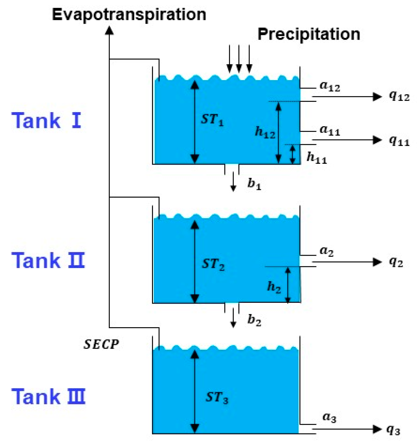
There are many different possible configurations of a Tank model depending on the number of storage (tanks or layers) and the locations of outlets. The 3-Tank model is one of the most common forms of a Tank model; it represents the hydrological processes of a watershed with the help of three tanks (or storages) that are vertically connected with outlets located at the bottom and side of each tank (Figure 1) [8,9,36]. The height of the side-outlets and the size of each tank are calibrated to observed streamflow so that the model can predict the overall watershed responses to rainfall events. In the model, water running out of the side outlets of the first tank (or the top layer), second tank, and third tank (or the bottom layer) represents surface runoff, intermediate runoff, and baseflow, respectively [8,9,13]. Water passing through the bottom outlets means infiltration (from the first tank to the second) or percolation (from the second tank to the third). The amount of runoff or infiltrated/percolated water through the outlets is assumed to be linearly proportional to the storage of a Tank as follows (Equations (1) and (2)):

$$Q_t=q_{11}+q_{12}+q_2+q_3={{\displaystyle \sum }}_{i=1}^n{{\displaystyle \sum }}_{j=1}^m{a}_{ij}\times \left(S{T}_{i,t}-h_{ij}\right),$$

(1)

$$I_{i,t}=b_i\times S{T}_{i,t},$$

(2)

where $i$ is the tank order, $j$ is the side-outlet order, $n$ is the number of tanks, $m$ is the number of side outlets for each tank, $q_{ij}$ is the runoff (mm) from the $j$th side outlet in the $i$th tank, $a_{ij}$ is the side-outlet coefficient (dimensionless) for the $j$th side-outlet in the $i$th tank, $S{T}_{i,t}$ is the storage of the $i$th tank (mm), $h_{ij}$ is the height of the side outlet for the $j$th side outlet in the $i$th tank (mm), $I_{i,t}$ is the amount of water infiltrated in the $i$th tank (mm), and $b_i$ is the bottom-outlet coefficient (dimensionless) for the $i$th tank. The $S{T}_{i,t+1}$ in the tanks, the storage for the next time step $t+1$, can be expressed as follows (Equations (3) and (4)):

$$S{T}_{i,t+1}=S{T}_{i,t}+P_{t+1}-E{T}_{i,t+1}-I_{i,t}-q_{i,t} \mathrm{for} i=1,$$

(3)

$$S{T}_{i,t+1}=S{T}_{i,t}+I_{i-1,t}-E{T}_{i,t+1}-I_{i,t}-q_{i,t} \mathrm{for} i=2, 3,$$

(4)

where $P_t$ is the precipitation at time $t$ (mm), and $E{T}_{i,t}$ is the actual evapotranspiration of the $i$th tank at time $t$ (mm). The $E{T}_{i,t}$ is constrained by the volume of storage in each tank (Equations (5) and (6)). It is calculated by subtracting the evapotranspiration in the upper tanks from the total actual evapotranspiration ($E{T}_{a,t}$):

$$E{T}_{i,t}=S{T}_{i,t} \mathrm{for} E{T}_{i,t}\ge S{T}_{i,t},$$

(5)

$$E{T}_{i,t}=E{T}_{a,t}-{{\displaystyle \sum }}_{j=1}^{i-1}E{T}_{j,t} \mathrm{for} E{T}_{i,t}<S{T}_{i,t}.$$

(6)

The $E{T}_a$ was estimated using the guidelines of the Food and Agriculture Organization of the United Nations (FAO) as follows ([48]; Equation (7)):

$$E{T}_{a,t}=K_{c,t}\times K_{s,t}\times E{T}_{0,t},$$

(7)

where $K_{c,t}$ is the single crop coefficient (dimensionless), $K_{s,t}$ is the soil water stress coefficient ($K_{s,t}$) (dimensionless), and $E{T}_0$ is the potential evapotranspiration (mm), which was estimated using the FAO Penman–Monteith (PM) approach with gauged solar radiation, air temperature, wind speed, and relative humidity [48]. The $K_{c,t}$ is determined with the area-weighted averages of crop coefficient values for different land uses [36,48]. The $K_s$ was calculated from the simulated total watershed storage ($S{T}_t$) and a modified power function as represented in Equation (8) [36,40]:

$$K_s=1-\exp \left(-SECP\times {{\displaystyle \sum }}_{i=1}^{n}S{T}_{i,t}\right),$$

(8)

where $SECP$ is a soil evaporation compensation parameter, which is positively correlated to $K_s$. The $SECP$ parameter has been reported to vary from 0.001 to 0.1, depending on watershed soil texture [8,40,49]. We adopted the feasible ranges of the Tank model parameters that were set considering the hydrological characteristics of Korean watersheds [8,36] (

Table 1. Value ranges of 3-Tank model parameters [8,36].

Parameter	Description	Min.	Max.
$a_{11}$	Side-outlet coefficient for the first side outlet in the first tank (dimensionless)	0.08	0.5
$a_{12}$	Side-outlet coefficient for the second side outlet in the first tank (dimensionless)	0.08	0.5
$h_{11}$	Height of side outlet for the first side outlet in the first tank (mm)	5	60
$h_{12}$	Height of side outlet for the second side outlet in the first tank (mm)	20	110
$b_1$	Bottom-outlet coefficient for the first tank (dimensionless)	0.1	0.5
$a_2$	Side-outlet coefficient in the second tank (dimensionless)	0.03	0.5
$h_2$	Height of side outlet in the second tank (mm)	0	100
$b_2$	Bottom-outlet coefficient for the second tank (dimensionless)	0.01	0.35
$a_3$	Side-outlet coefficient in the third tank (dimensionless)	0.003	0.03
$SECP$	Soil evaporation compensation parameter	0.001	0.1

Constraint: $h_{11}<h_{12}.$

).

2.1.2. Regionalization of the Tank Models

The Tank models have been widely employed as a tool to predict the streamflow of ungauged watersheds in Korea, Japan, and Germany [4,13,14,17,18,40,41] (

Table 2. An overview of previous studies related to the regionalization of Tank models.

Reference	Country	No. Tanks	No. Watersheds	Drainage Area (km2)	Period (Years)	Optimization Method	Objective Function	Dependent Variables
Yokoo et al. [17]	Japan	4	12	100–805	3	Powell method	$MRE$	Area (km2), representative gradient (%), percentage of three geology types (%), percentage of three soil types (%), percentage of eight land-use types (%)
Amiri et al. [4]	Germany	4	30	53–737	15	Marquardt algorithm	$MSE$	Percentage of three soil types (%), mean patch size of the water body patches (ha), mean shape index of mix forest patches (-), mean perimeter to area ratio of two land-use patches (m/ha), patch density of five land-use patches (No./ha)
Kim and Park [13]	Korea	3	12	0.5–140.5	1–2	Manual	$RMSE$	Area (km2), Forest (%), Upland (%), Paddy (%)
Huh et al. [40]	Korea	3	15	3–2060	3–10	Rosenbrock	$RMSE$	Area (km2), Length (km), Form (-), Forest (%), Upland (%), Paddy (%)
Kim et al. [41]	Korea	3	26	5.9–7126	7–10	Manual	NA	Area (km2), W_Slope (%), Length (km), Form (-), Forest (%), Upland (%), Paddy (%)
An et al. [18]	Korea	3	30	56–6662	5–36	Genetic Algorithm	$RMSE$	Area (km2), Length (km), W_Slope (%), Forest (%), Upland (%), Paddy (%)

$MRE$, $MSE$, and $RMSE$ refer to mean relative error, mean square error, and root mean square error, respectively. NA refers to information not available. W_Slope (%), Length (km), and Form (-) refer to the watershed slope, flow length, and form factor, respectively. Upland is an area where crops are cultivated under non-ponded conditions, and paddy is an area that can maintain a ponded water depth to grow rice. Forest (%), Upland (%), and Paddy (%) refer to the percentages of the forest, upland, and paddy area, respectively.

). The model parameters are estimated from the relationship between parameter values and watershed characteristics, which are developed using observations made in gauged watersheds. The Tank model was originally developed with four layers (4-Tank) [37], and the parameter values of the 4-Tank models were generally derived from selected watershed features in Japan and Germany [4,17].

Yokoo et al. [17] regionalized the 12 parameters of the 4-Tank model using flow measurements made in 12 watersheds that had drainage areas with a range from 100 to 805 km² in Japan; the watershed characteristics were derived from topography, soil type, geology, and land-use. In their study, a multiple linear regression model successfully identified the statistical relationship between the model parameters and the watershed characteristics. Amiri et al. [4] examined whether changes in landscape metrics, including shape index, perimeter-area ratio, patch size, and patch density of land-use, could affect the calibrated values of the 4-Tank model parameters from 30 catchments (53–737 km²) located in Germany. They found that multiple regression models could successfully explain the relationship between calibrated parameter values and a highly varying landscape, and landscape metrics should be included in the regionalization of conceptual rainfall-runoff models.

In Korea, a three-layer Tank model, modified with two side outlets on the top layer, has been widely employed, especially to study small- or medium-sized watersheds where flow travel time is short, and the recession limb of a streamflow hydrograph is steep [9,36]. Various regionalization approaches have been carried out in Korea to estimate ungauged streamflow [13,18,40,41]. Kim and Park [13] developed regression equations to estimate reservoir inflow in ungauged watersheds using only the information of drainage area and land-use composition. Similarly, Huh et al. [40], Kim et al. [41], and An et al. [18] considered the topographical characteristics, such as stream length, slope, and form factor when developing the regression relationship.

2.2. Model Calibration and Evaluation

2.2.1. Objective Functions

Two objective functions were employed in the parameter calibration to see how the selection of objective functions could affect the regionalization of the Tank model: $RMSE$ and modified $KGE$ ($KGE{\prime }_{sqrt}$) [45,46]. The $RMSE$ (mm), which is relatively responsive to high flow or peak flow, has been widely used for calibrating hydrological models (Equation (9)):

$$RMSE=\sqrt{\frac{{{\displaystyle \sum }}_{i=1}^n{\left(O_i-S_i\right)}^2}{n}},$$

(9)

where $O$ and $S$ represent the observed and simulated discharge (mm), respectively, $n$ is the number of time steps at a time step $i$. The $KGE$ was proposed as an alternative performance statistics [45]. The modified version, $KGE\prime$, was introduced to ensure that the bias and variability ratios are not cross-correlated to take into account the multiple aspects of model evaluation, including correlation, bias, and variability simultaneously [46]:

$$KGE=1-\sqrt{{\left(r-1\right)}^2+{\left(\beta -1\right)}^2+{\left(\alpha -1\right)}^2},$$

(10)

$$KGE\prime =1-\sqrt{{\left(r-1\right)}^2+{\left(\beta -1\right)}^2+{\left(\gamma -1\right)}^2},$$

(11)

$$r=\frac{cov\left(O,S\right)}{{\sigma }_O{\sigma }_S},$$

(12)

$$\beta =\frac{{\mu }_S}{{\mu }_O},$$

(13)

$$\alpha =\frac{{\sigma }_S}{{\sigma }_O},$$

(14)

$$\gamma =\frac{{\mu }_O{\sigma }_S}{{\sigma }_O{\mu }_S},$$

(15)

where $r$ is the Pearson correlation coefficient between simulated and observed streamflow (dimensionless), $\beta$ is the bias ratio (dimensionless), $\alpha$ is the standard deviation ratio (dimensionless), $\gamma$ is the variability ratio (dimensionless), $cov$ is the covariance between observation and simulation, $\mu$ is the mean runoff (mm or cms), and $\sigma$ is the standard deviation (mm or cms). As the modified $KGE\prime$ tends to be sensitive to large values, a square root transformation (or the Box-Cox power transformation with a lambda value of 0.5) ($KGE{\prime }_{sqrt}$) was applied to the original flow before computing $KGE\prime$ to reduce the degree of expected bias toward high flow [8,47].

2.2.2. The Automatic Parameter Calibration Algorithm

Automatic calibration with selected objective functions was performed by the shuffled complex evolution algorithm (SCE), which is a sampling-based heuristic search strategy [50,51]. Previous studies have proved its applicability to the calibration of hydrological models [8,45,46,52], and the details of SCE are well described in literature [50,53]. The SCE sampling of this study employed 15 complexes and 21 points (or populations) per complex. The sampling continued until the differences between the objective function values sampled in the last 10 points were less than 0.1%.

2.2.3. Model Evaluation Statistics

The calibrated Tank models were evaluated using four performance statistics commonly used in hydrological modeling: (1) $NSE$ [42], (2) a log-transformed $NSE$ ($NS{E}_{ln}$) [34], (3) percent bias ($PBIAS$) [51], and (4) flow duration curve (FDC) index ($NSEFDC$) [8,54]. The $NSE$ is known as a sensitive index to high flow, and it was used to evaluate high flow accuracy [54,55]. The $NS{E}_{ln}$ has an increased influence of low values as compared to the original $NSE$ because of the logarithm, and thus it was employed to access low flow simulation [8,34,54]. The $NSEFDC$ is a type of Nash–Sutcliffe efficiency designed to measure the similarity between FDCs [8,54,56], indicating the flow variability index. The values of $NSE$, $NSEln$, and $NSEFDC$ are close to 1 when there is a complete agreement between simulated and observed streamflow, but they can become large negative values ($-\infty$) when the discrepancy between them is wide. The measures the overall tendency or bias that the simulated data have compared to the observed [57]. More detailed equations of $NSE$, $NS{E}_{ln}$, $NSEFDC$, and $PBIAS$ can be seen in [8].

2.3. Relating Watershed Characteristics to Model Parameter Values

Multiple linear regression was carried out to find out the regression relationship between the calibrated Tank model parameter values (dependent variables) and watershed characteristics (independent variables):

$$y_i={\beta }_0+{\beta }_1{x}_1+{\beta }_2{x}_2+\dots +{\beta }_{n-1}{x}_{n-1}+{\epsilon }_i,$$

(16)

where y_i is the calibrated parameter of the Tank model, x₁, $x_2, \dots$, $x_{n-1}$ are the watershed characteristics, including surface geology and land use types, β₀, ${\beta }_1$, …, ${\beta }_{n-1}$ are coefficients, and ε_i is a model constant [58]. The logarithmic transformation for independent variables was considered to explore the best regression model. Three strategies of variable selection methods, forward, backward, and stepwise selections, were employed to determine the optimum number of independent variables; the strategy that provided the highest adjusted $R^2$ was finally selected. No more than five independent variables were used in each regression.

3. Study Watersheds and Their Characteristics

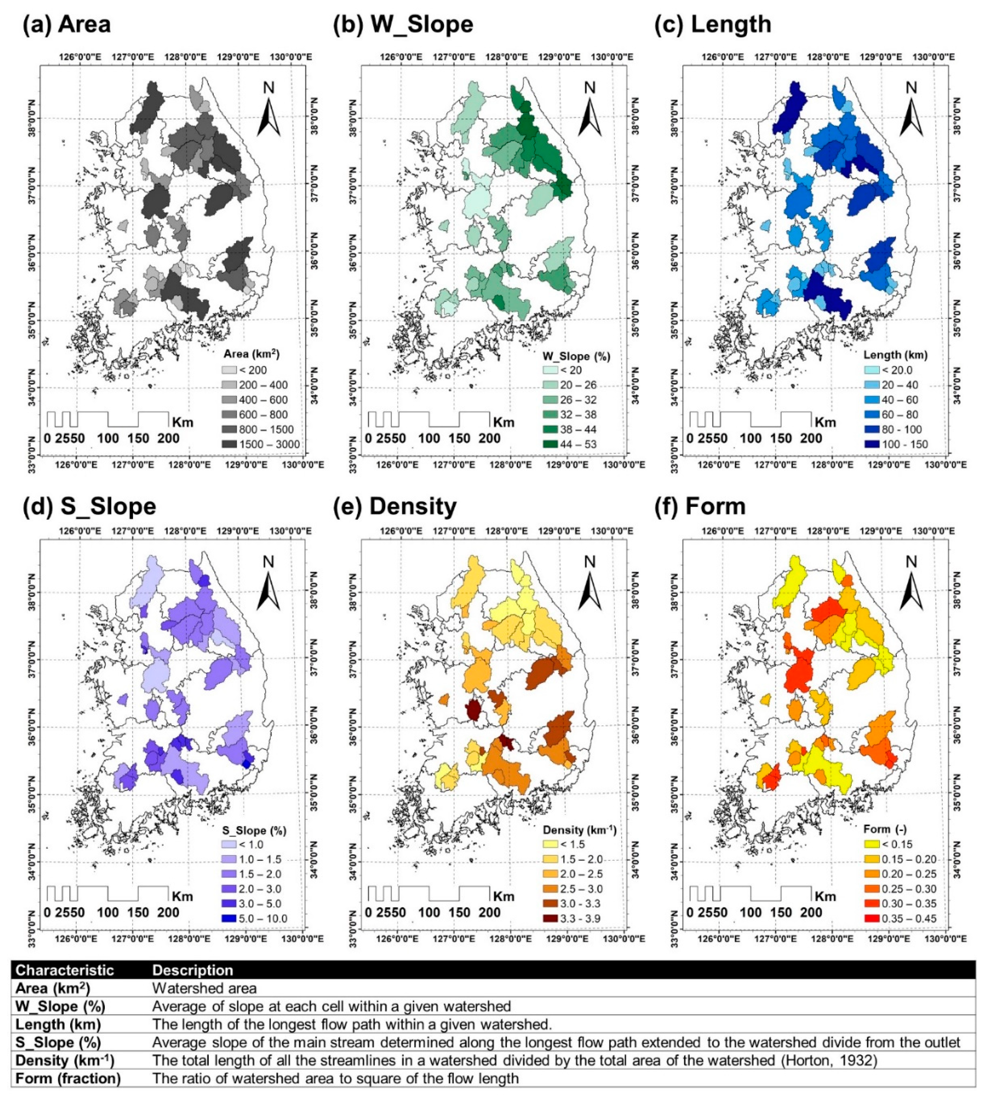
Forty-nine watersheds draining 3.8 to 2990.7 km² throughout South Korea were selected on the basis of the variability of their locations, land uses, and topography in this study [8,59] (Figure 2). The study watersheds represent a wide range of hydrological conditions, such as drainage areas (Area), watershed and channel slopes (W_Slope and S_Slope), drainage densities (Density) [60], flow lengths (Length), form factors (Form), and the percentages of forest (Forest), rice paddy fields (Paddy), and uplands (Upland) (Figure 2). These watersheds were randomly divided into two groups. The first group included 39 watersheds to be used in the development of the regional equations. The second group consisted of 10 watersheds to be used to verify the developed regression equations.

The precipitation records of weather stations associated with the study watersheds were obtained from the Korea Meteorological Administration (KMA), and the areal average precipitation was determined using the Thiessen polygon method [61]. Other daily weather variables, including temperature, relative humidity, mean wind velocity, and solar radiation, were obtained from the KMA and used to calculate the potential evapotranspiration (PET) by the FAO-PM method [48]. Topographic characteristics, including drainage area, watershed mean slope, channel slope, drainage density, flow length, and form factor, were calculated using 30-m digital elevation models (DEMs) provided by the National Geographic Information Institute (NGII). The percentages of forest, upland, and paddy areas were calculated from a land-use map obtained from the Ministry of Environment (MOE).

Observed daily streamflow data of the study watersheds were compiled from the Korea Ministry of Land, Infrastructure, and Transport (MOLTM) and Seoul National University [59,62]. The length of available flow records varies from one watershed to another, and all study watersheds included at least five years of data. A split sample test scheme was employed to calibrate and validate the models; at least three and two years of streamflow records were used for calibration and validation, respectively. In addition, the calibration periods were set to include wet, average, and dry years [63,64]. The first two years of weather records were used to stabilize the hydrological variables of the model so that calibration results would be minimally affected by arbitrary and rough assumptions made for the initial conditions. In this study, the parameters of 3-Tank models were calibrated to streamflow observations made at the outlets of the 39 study watersheds with two different objective functions, $RMSE$ and $KGE{\prime }_{sqrt}$ (Table 1 and Figure 2).

4. Results and Discussion

4.1. Parameter Calibration

We defined the $optRMSE$ and ${optKGE\prime }_{sqrt}$ as the cases of using $RMSE$ and ${KGE\prime }_{sqrt}$ as an objective function, respectively. The performance statistics were compared in terms of high and low flow, FDC, and runoff volume. The statistical significance of differences between the model performance statistics was investigated using a paired t-test at a significance level of 0.05.

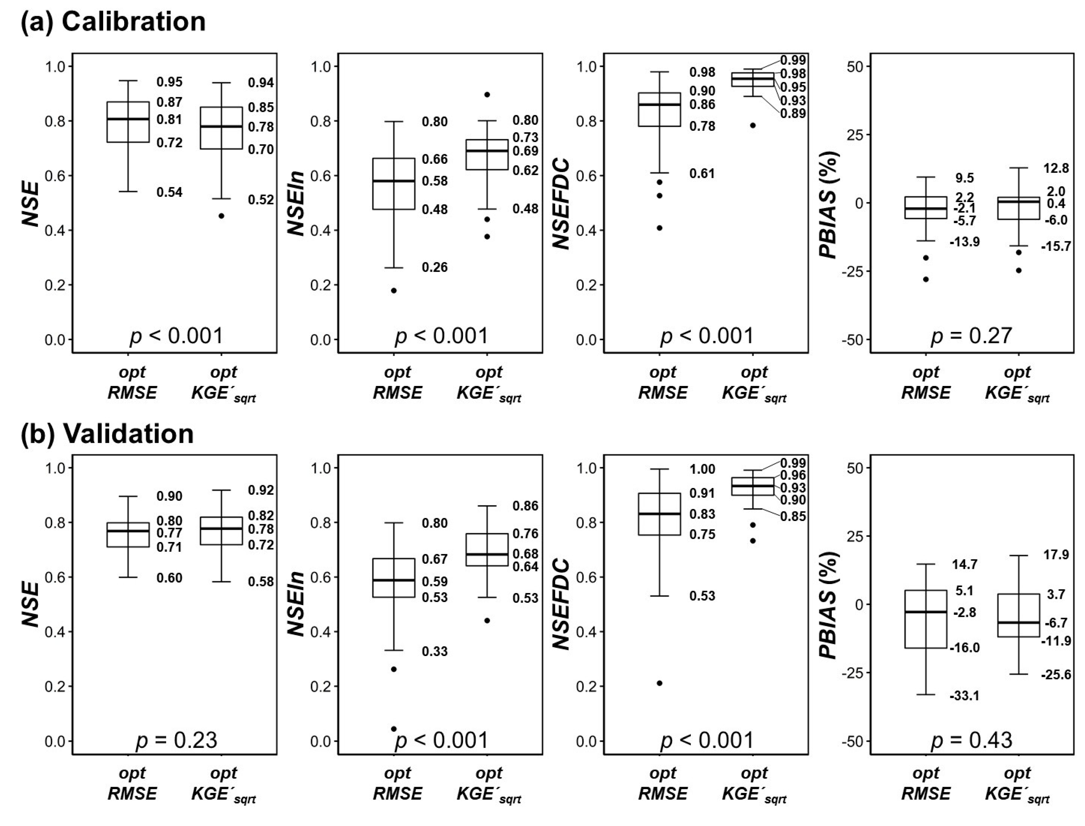
Overall, the parameter calibration provided satisfactory performance in most study watersheds, especially in the case of the ${optKGE\prime }_{sqrt}$ (

Table 3. Performance comparison of the 3-Tank model calibrated with the two objective functions ($optRMSE$ and $optKGE{\prime }_{sqrt}$) for the 39 study watersheds.

Period	Model	Performance
		Unsatisfactory	Satisfactory
			Fine a	Good b	Very Good c	Total
Calibration	$optRMSE$	5%	36%	33%	26%	95%
	$optKGE{\prime }_{sqrt}$	10%	28%	31%	31%	90%
Validation	$optRMSE$	28%	31%	28%	13%	72%
	$optKGE{\prime }_{sqrt}$	15%	46%	26%	13%	85%

^a Fine: $0.50<NSE\le 0.70$, and ±10 ≤ $PBIAS$ < ±15. ^b Good: $0.70<NSE\le 0.80$, and ±5 ≤ $PBIAS$ < ±10. ^c Very good: $NSE>0.80$, and $PBIAS$ < ±5.

). The $optRMSE$ yielded slightly higher $NSE$ values (or more accurate peak flow prediction) than ${optKGE\prime }_{sqrt}$ in the calibration of the 3-Tank model parameters (p < 0.001) (Figure 3). However, the differences between the $NSE$ values were not statistically significant in the validation ($p$ > 0.05). The use of ${KGE\prime }_{sqrt}$ provided significantly better accuracy in predicting low flow ($NSEln$) and flow variability ($NSEFDC$) as compared to that of $optRMSE$ ($p$ < 0.001). In terms of $PBIAS$ (or the overall water balance), the two objective functions provided no significant difference for both evaluation periods ($p$ > 0.05). Such results imply that $optKGE{\prime }_{sqrt}$ can provide more balanced evaluation aspects than $optRMSE$ in model parameter calibration, as $KGE$ is more responsive to low values than $RMSE$ [8,45,47]. In this study, we included study watersheds where the corresponding models provided “satisfactory” performance (0.50 < $NSE$ and $PBIAS$ < ±15) so that we could exclude the influence of models that do not apply to the watersheds on parameter regionalization.

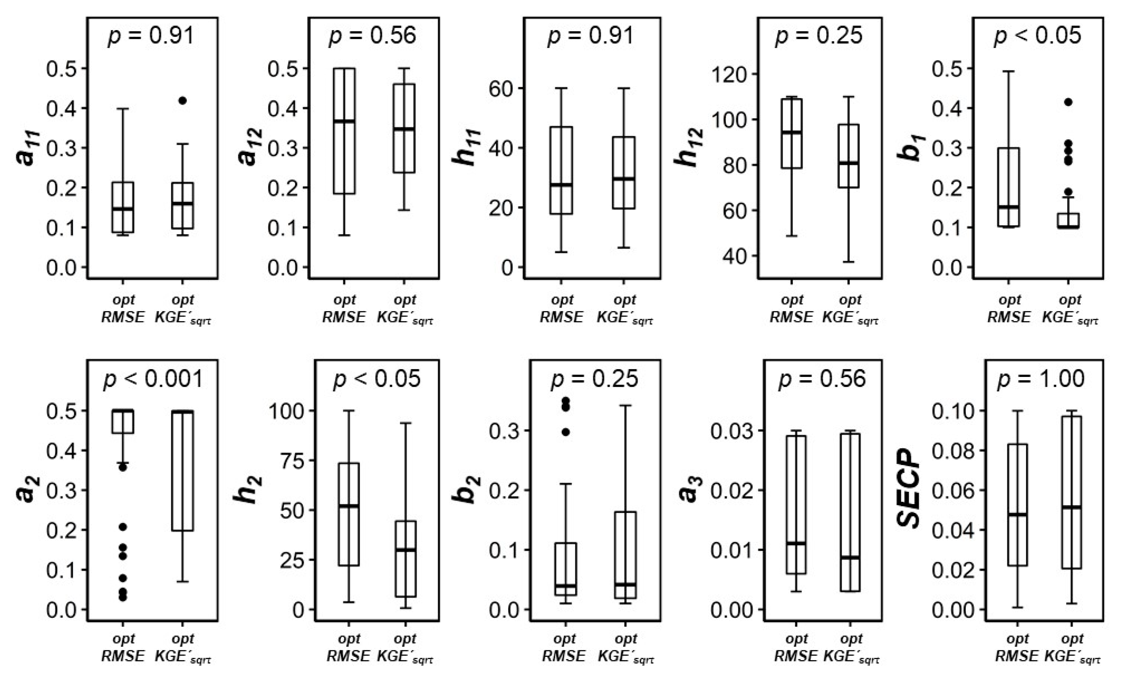
The Kolmogorov–Smirnov (KS) test was conducted to see if there are statistically significant differences in the parameter value distributions of the 3-Tank models calibrated with $RMSE$ and $KG{E}_{sqrt}$ (at the significance level of 0.05). The comparison showed that the use of different objective functions provided the distributions of $b_1$, $a_2$, and $h_2$ that were significantly different from each other ($p$ < 0.05) (Figure 4). Furthermore, $b_1$ controlled the amount of water that infiltrated through the bottom outlet of the top tank into the second layer, and $a_2$ and $h_2$ regulated the amount of intermediate runoff; thus the three parameters were critical to the shapes of recession and baseflow parts of the streamflow hydrographs. Such findings indicate that the selection of an objective function in model calibration can substantially influence the hydrological analyses, including regionalization, by providing different mathematical representations for a watershed under consideration and by creating parameter uncertainty. In the following sections, we have demonstrated how the objective function selection can influence the regionalization of model parameters and their uncertainty.

4.2. Regionalization

4.2.1. Regionalization of the 3-Tank Model

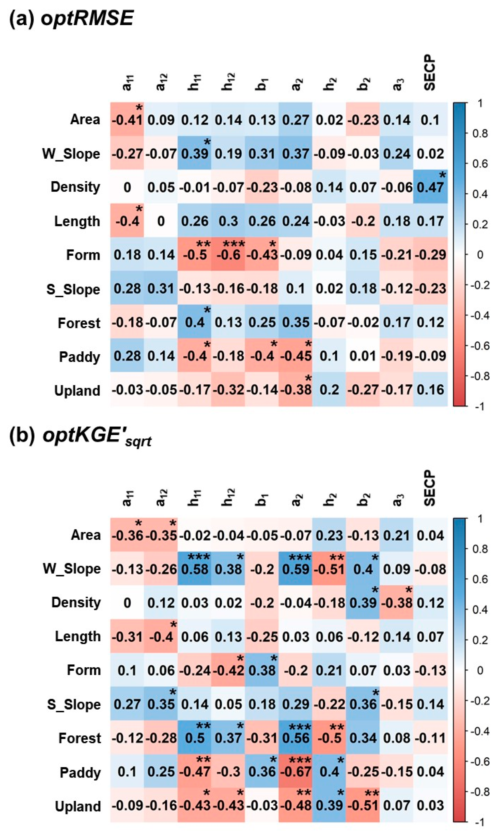
The correlation structure between calibrated parameter values and selected hydrologic features of the watersheds was investigated to identify key watershed characteristics (Figure 5). At least six of the parameters were correlated ($\left|r\right|\ge 0.4$, $p<0.05$) to one or more of the watershed features. The five parameters that were associated with the first layer (or the top tank) of the 3-Tank model, including $a_{11}$, $a_{12}$, $h_{11}$, $h_{12}$, and $b_1$, turned out to be correlated to topographic factors, such as W_Slope, Length, S_Slope, and Form. Such a correlation structure was expected, as the first layer of a Tank model is usually introduced to simulate hydrological processes happening on the ground surface, such as direct runoff generation and routing [8,9,13].

In the case of using the objective function of $RMSE$, close correlation structures ($0.7> \left|r\right|>0.5$, $p<0.01$) were found in between Form and the heights of two side outlets of the first layer, $h_{11}$ and $h_{12}$ (Figure 5). When $KGE{\prime }_{sqrt}$ was employed as the objective function, however, $h_{11}$ showed a close relationship with W_Slope ($r=0.58$, $p<0.001$), and $h_{12}$. was associated with Form ($r=-0.42$, $p<0.05$) and Upland ($r=-0.43$, $p<0.05$). The outlet heights, $h_{11}$ and $h_{12}$, of the first layer control the quick runoff response and high (and peak) flow of a watershed, respectively, and they control the surface storage capacity at the beginning of an event ($h_{11}$) and the total surface storage capacity ($h_{12}$) of the upper layer [8,17,37,65]. Thus, the findings imply that direct runoff of the study watersheds is relatively heavily controlled by Form, W_Slope, and Upland than the other watershed features, which is corroborated by our understanding and previous studies [8,66,67,68].

The parameters of the second tank ($a_2$, $h_2$, and $b_2)$ and third tank ($a_3$) determine the shapes of recession and baseflow-only parts of a streamflow hydrograph [8]. The calibrated values of $a_2$ are relatively strongly correlated to Paddy, regardless of the types of objective functions. In the case of calibrating with $KGE{\prime }_{sqrt}$, $h_2$ was found to be correlated to W_Slope ($r=-0.51$, $p<0.01$) or Forest ($r=-0.50$, $p<0.01$), and $b_2$ was also correlated to Upland ($r=-0.51$, $p<0.01$). The calibrated values of $a_3$ were associated with Density ($r=-0.38$, $p<0.05$) when $KGE{\prime }_{sqrt}$ was used as the objective function; however, the parameter did now show any statistically significant relationship with the watershed characteristics in the case of the $RMSE$ objective function.

4.2.2. Performance of the Regionalized 3-Tank Models

The two regional models ($regRMSE$ and $regKGE{\prime }_{sqrt}$) were developed by relating the calibrated values of parameters to the watershed characteristics (

Table 4. The 3-Tank model parameters regionalized based on the results of calibration implemented with $optRMSE$.

Par.	Equations	R2	$\mathit{A}\mathit{d}\mathit{j}.{\mathit{R}}_2$
$a_{11}$	0.123
$a_{12}$	0.364
$h_{11}$	$54.841-109.254\times \mathrm{Form}(-)$	0.25	0.22
$h_{12}$	$-26.734-290.122\times \mathrm{Form}(-)+15.157\times \mathrm{S}\_\mathrm{slope}(\%)+2.346\times \mathrm{Paddy}(\%)+30.219\times \ln \left(\mathrm{Length}\left(\mathrm{km}\right)\right)$	0.66	0.60
$b_1$	$-0.0352-0.210\times \ln \left(\mathrm{Area}\left({\mathrm{km}}^2\right)\right)+0.403\times \ln \left(\mathrm{Length}\left(\mathrm{km}\right)\right)$	0.23	0.17
$a_2$	$0.5305-0.0097\times \mathrm{Paddy}(\%)$	0.20	0.17
$h_2$	46.2
b2	0.061
a3	0.007
$SECP$	−0.0143 + 0.0283 × Density(km−1) − 0.1235 × Form(−) + 0.0061 × ln⁡(Area(km2))	0.40	0.33

and

Table 5. The 3-Tank model parameters regionalized based on the results of calibration implemented with $optKGE{\prime }_{sqrt}$.

Par.	Equations	${\mathit{R}}_2$	$\mathit{A}\mathit{d}\mathit{j}.{\mathit{R}}_2$
$a_{11}$	0.168
$a_{12}$	$\begin{array}{c}1.9032-0.0074\times \mathrm{W}\_\mathrm{slope}(\%)-1.9193\times \mathrm{Form}(-)-0.0114\times \mathrm{Upland}(\%)\\ +0.3082\times \ln (\mathrm{Area}\left({\mathrm{km}}^2\right))-0.7034\times \ln \left(\mathrm{Length}\left(\mathrm{km}\right)\right)\end{array}$	0.45	0.35
$h_{11}$	$1.828+0.957\times \mathrm{W}\_\mathrm{slope}(\%)$	0.33	0.31
$h_{12}$	$119.514-91.270\times \mathrm{Form}(-)-2.235\times \mathrm{Upland}(\%)$	0.32	0.27
$b_1$	0.100
$a_2$	$0.9087-0.0180\times \mathrm{Paddy}(\%)-0.0805\times \ln \left(\mathrm{Length}\left(\mathrm{km}\right)\right)$	0.57	0.54
$h_2$	$123.027-8.223\times \mathrm{Density}\left({\mathrm{km}}^{-1}\right)-0.962\times \mathrm{Forest}(\%)-9.786\times \ln \left(\mathrm{S}\_\mathrm{slope}(\%)\right)$	0.37	0.30
$b_2$	$-0.0486+0.0028\times \mathrm{W}\_\mathrm{slope}(\%)+0.0649\times \mathrm{Density}\left({\mathrm{km}}^{-1}\right)-0.0108\times \mathrm{upland}(\%)$	0.48	0.42
$a_3$	$\begin{array}{c}0.05104+0.00077\times \mathrm{W}\_\mathrm{slope}(\%)-0.00270\times \mathrm{Density}\left({\mathrm{km}}^{-1}\right)+0.06569\\ \times \mathrm{Form}(-)-0.00814\times \ln (\mathrm{Area}\left({\mathrm{km}}^2\right))-0.02560\\ \times \ln \left(\mathrm{S}\_\mathrm{slope}(\%)\right)\end{array}$	0.42	0.31
$SECP$	0.0470

). Regression equations were assigned to parameters that were at least “moderately” ($\left|r\right|\ge 0.35$) correlated to any of the watershed features. When the correlation structure between the parameter values and watershed features was weak ($\left|r\right|<0.35$), the median of the parameter values that had been calibrated to individual study watersheds was used to represent the overall average value of the parameter [15]. When $KGE{\prime }_{sqrt}$ was used as the objective function in the calibration, stronger correlation structures were found between the parameter values and watershed characteristics as compared to the $optRMSE$ (Figure 5, Table 4 and Table 5).

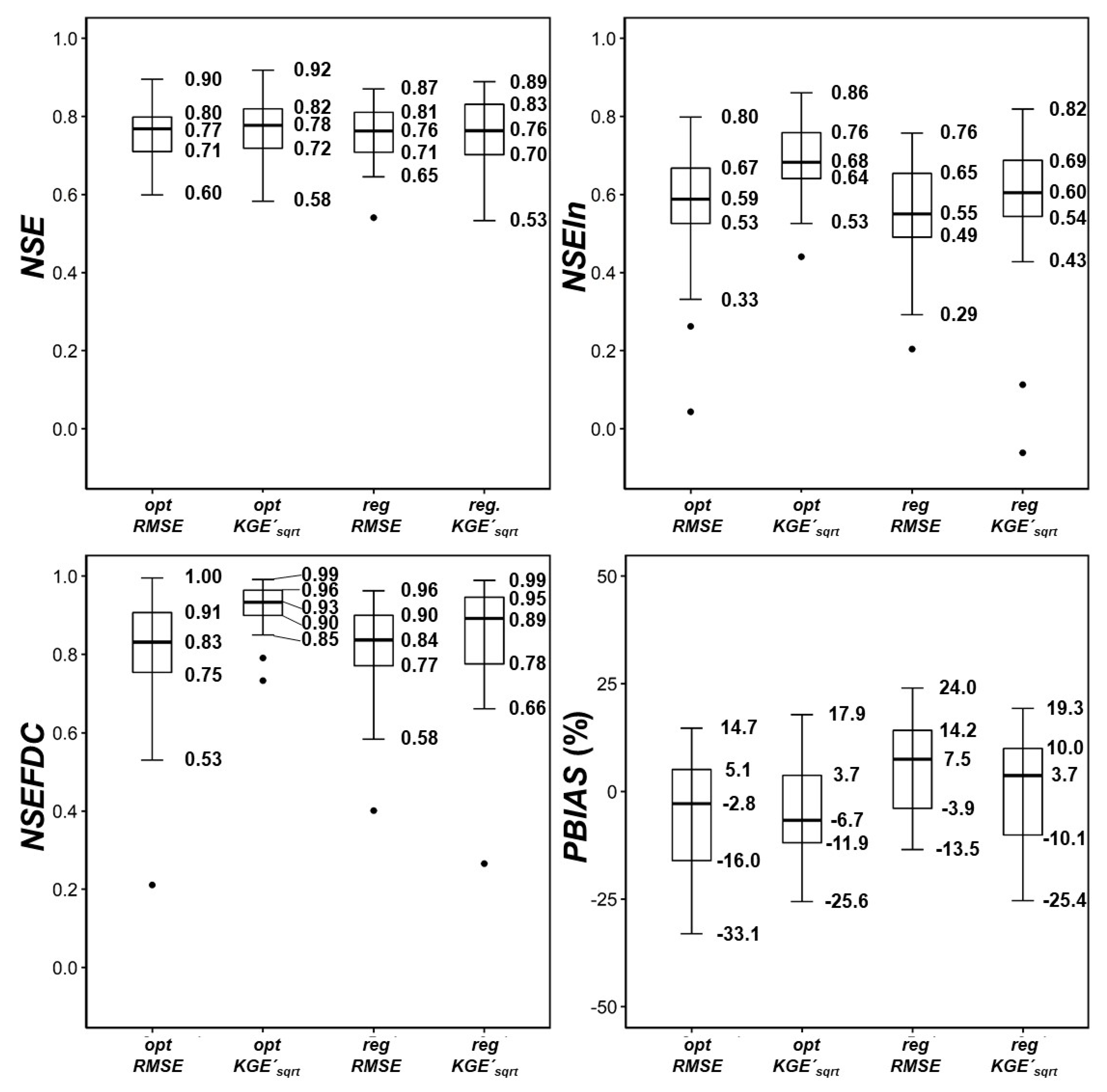
The accuracy of the regionalized 3-Tank models was evaluated by comparing the model performance statistics provided by the calibrated and regionalized models for the 39 study watersheds employed in the regionalization (Figure 6). A one-way analysis of variance (ANOVA) was carried out to determine the statistical significance of differences between the performance statistics of the four groups ($optRMSE$, $optKGE{\prime }_{sqrt}$, $regRMSE$, and $regKGE{\prime }_{sqrt}$). Subsequently, a post-hoc Tukey honest significant difference (HSD) test was performed to facilitate a pairwise comparison of the performance statistics provided by the models [8,69].

Overall, the two regionalized models ($regRMSE$ and $regKGE{\prime }_{sqrt}$) provided similar accuracy to that of the calibrated models ($optRMSE$ and $optKGE{\prime }_{sqrt}$). There was no statistically significant difference between the $NSE$ values achieved by the four models ($p>0.05$), which implied that regionalization can predict high (or peak) flow at the level of accuracy similar to those of the calibrated models. In terms of $NS{E}_{ln}$ and $NSEFDC$, however, $regKGE{\prime }_{sqrt}$ yielded better performance than the $regRMSE$, presumably because $optKGE{\prime }_{sqrt}$ yielded better accuracy than regRMSE ($p<0.01$). However, $optKGE{\prime }_{sqrt}$ and $regKGE{\prime }_{sqrt}$ provided similar accuracy ($p>0.05$). The $regRMSE$ slightly underestimated the overall runoff volume (e.g., positive $PBIAS$) as compared to $regKGE{\prime }_{sqrt}$; this may be attributed to $KGE{\prime }_{sqrt}$ providing more balanced views on model performance than the $RMSE$ [8,45,47].

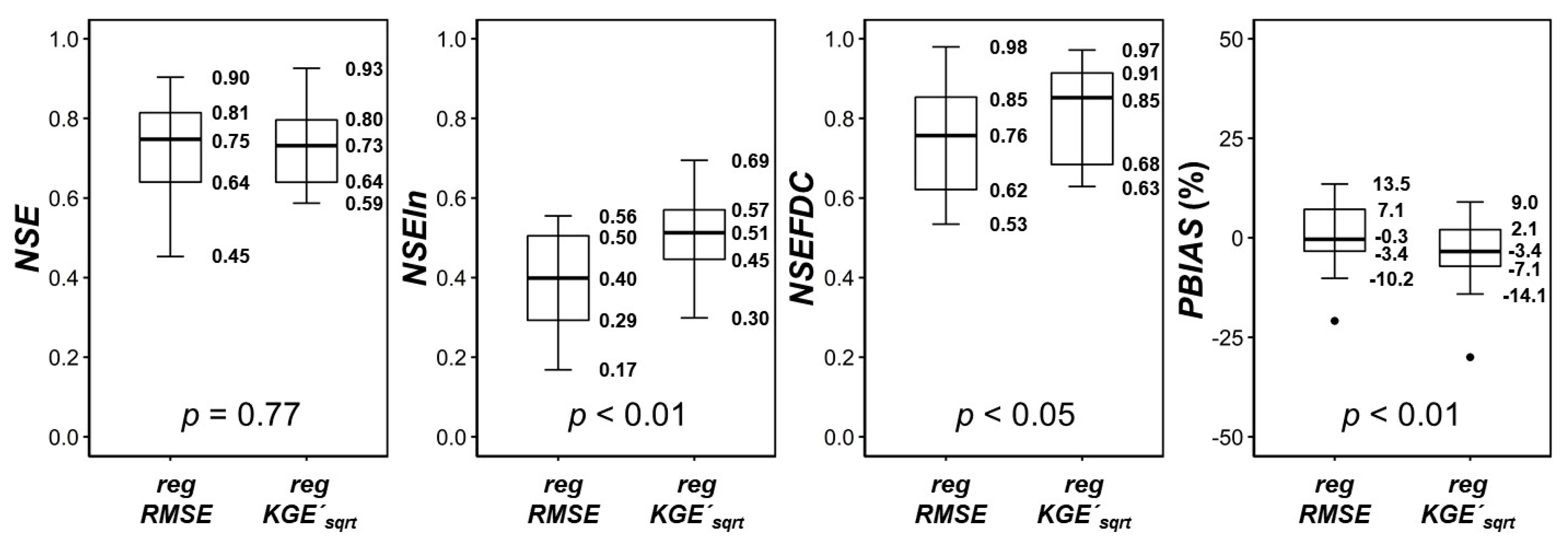
The performance of the regionalized models ($regRMSE$ and $regKGE{\prime }_{sqrt}$) was further investigated by applying them to the other 10 study watersheds that were not used in the regionalization processes (Figure 7). The sample size was small ($n=10$); therefore, the non-parametric Wilcoxon signed-rank test was conducted to test the significance of any differences between the performance statistics provided by the two regionalized models at a significance level of 5%. The $regKGE{\prime }_{sqrt}$ model yielded $NS{E}_{ln}$, $NSEFDC$, and $PBIAS$ significantly better than those of $regRMSE$ while they provided statistically similar $NSE$ values. Such results highlight the potential of $regKGE{\prime }_{sqrt}$ as a strategy for RR model regionalization.

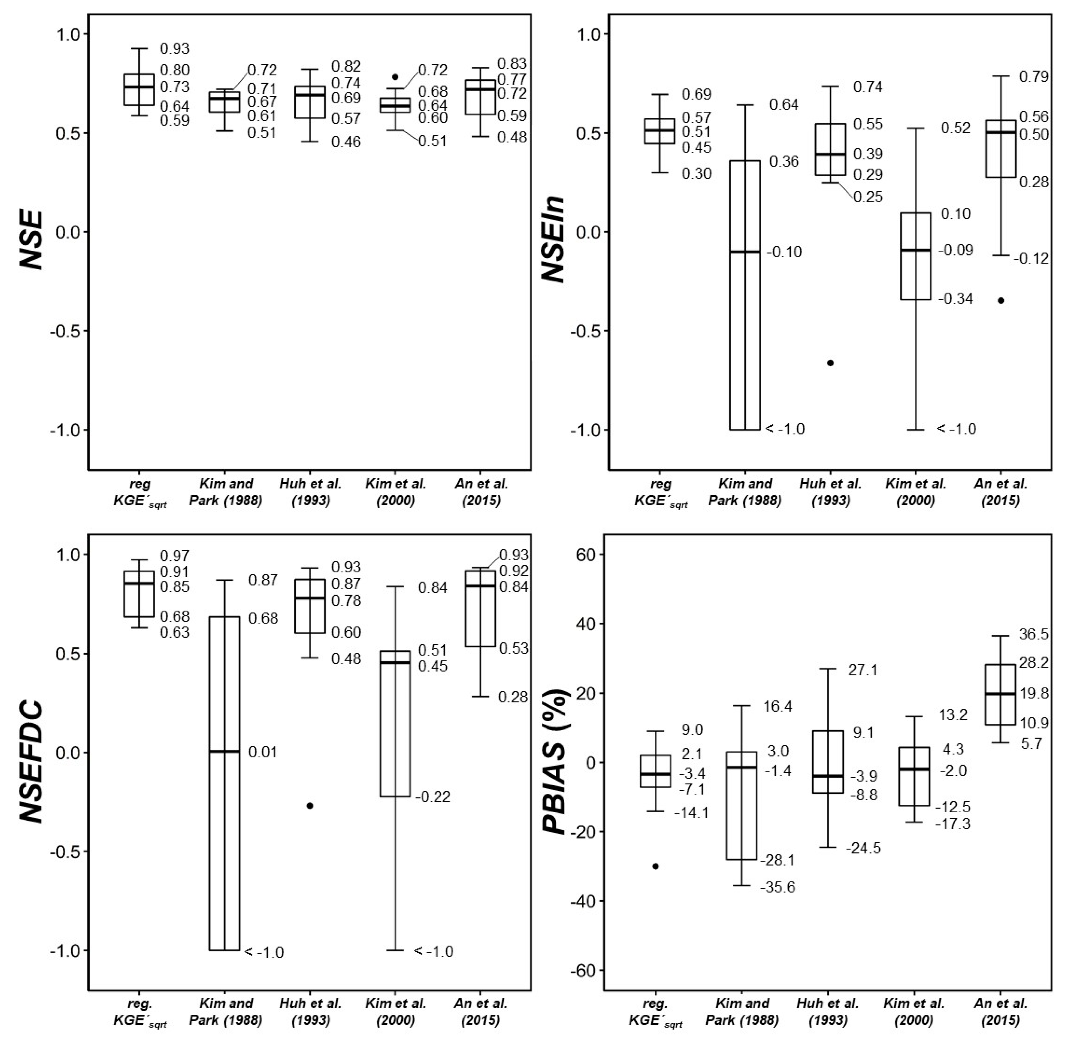
The performance of the two models was compared with that of other regionalized models using the 10 validation watersheds (

Table 6. Comparison of the performance of the two regional models ($regRMSE$ and $regKGE{\prime }_{sqrt}$) and others prepared for the 10 validation watersheds.

Model	Performance
	Unsatisfactory	Satisfactory
		Fine a	Good b	Very Good c	Total
$regRMSE$	20%	50%	10%	20%	80%
$regKGE{\prime }_{sqrt}$	10%	60%	20%	10%	90%
Kim and Park [13]	50%	30%	20%	0%	50%
Huh et al. [40]	40%	40%	20%	0%	60%
Kim et al. [41]	20%	70%	10%	0%	80%
An et al. [18]	70%	0%	30%	0%	30%

^a Fine: $0.50<NSE\le 0.70$, and ±10 ≤ $PBIAS$ < ±15. ^b Good: $0.70<NSE\le 0.80$, and ±5 ≤ $PBIAS$ < ±10. ^c Very good: $NSE>0.80$, and $PBIAS$ < ±5.

). As seen in the comparison, the two models regionalized in this study outperformed the others in terms of $NSE$ and $PBIAS$. The 3-Tank models regionalized by Kim et al. [41] provided a performance that was comparable to that of this study. However, An et al. [18] reported relatively poor performance as compared to others. We applied one-way ANOVA and HSD tests to see if there were significant differences between the performance statistics provided by the 3-Tank models regionalized for the 10 validation watersheds (Figure 8).

The five regionalized models employed different regression equations that explained the relationships between parameter values and watershed characteristics, but there was no statistically significant difference between the $NSE$ values provided by them ($p>0.05$). In terms of $NSEln$ and $NSEFDC$, however, $regKGE{\prime }_{sqrt}$ provided significantly better performance as compared to ones that had been developed in Kim and Park [13] and Kim et al. [41]. The 3-Tank model regionalized by An et al. [18], yielded $NSEln$ and $NSEFDC$ values similar to those by $regKGE{\prime }_{sqrt}$ ($p>0.05$), but the model significantly underestimated runoff volume (positive $PBIAS$) compared to the other models ($p<0.05$). The regionalized model of Huh et al. [40] provided a level of efficiency similar to that of $regKGE{\prime }_{sqrt}$, but $regKGE{\prime }_{sqrt}$ outperformed the model in terms of the model evaluation criteria that are commonly employed in hydrological modeling practices [57] (Table 6).

The relatively worse performances of the models reported by Kim and Park [13] and Kim et al. [41], reproducing low flow, might be related to the models being developed on manually calibrated parameters; thus, the local optima could be used for regionalization (Table 2). In addition, the studies did not calibrate models by considering low flow efficiencies in the development process. Huh et al. [40] and An et al. [18] employed automatic optimizations (Table 2), and their models provided better low flow performances. However, the models produced relatively worse performances as compared to $regKGE{\prime }_{sqrt}$ as these studies used $RMSE$ as an objective function (Table 2), which may yield less balanced results than the case when $KGE{\prime }_{sqrt}$ is used.

In this study, we compared the prediction performance of two regionalized 3-Tank models that were calibrated with two different objective functions, $optRMSE$ and $optKGE{\prime }_{sqrt}$. From the comparison, we found that the models could predict high flow and water balance of the 49 study watersheds at acceptable levels of accuracy (Table 6, Figure 6, Figure 7 and Figure 8). We also saw that the use of $RMSE$ that has been widely employed as an objective function in the regionalization studies provided relatively poor performance in reproducing low flow and FDC compared to the use of $KGE{\prime }_{sqrt}$. Such a result is not surprising because $KGE{\prime }_{sqrt}$ considers flow variability more explicitly when evaluating model accuracy while $NS{E}_{sqrt}$ is still sensitive to peak or high flow [47]. It is worth noting that $optKGE{\prime }_{sqrt}$ gained significantly higher $NSEln$ and $NSEFDC$ values but slightly lower $NSE$ efficiency as compared to $optRMSE$ (Figure 3). Such a finding suggests that when low flow is one of the modeling outputs of interest, we should not solely rely on statistics including $NSE$ and $R^2$ that have been commonly used but also know that the statistics are very sensitive to high flow. Instead, combining alternative statistics, such as $NSEln$ and $NSEFDC$, could provide a balanced view point to model evaluation [8,9,55,70].

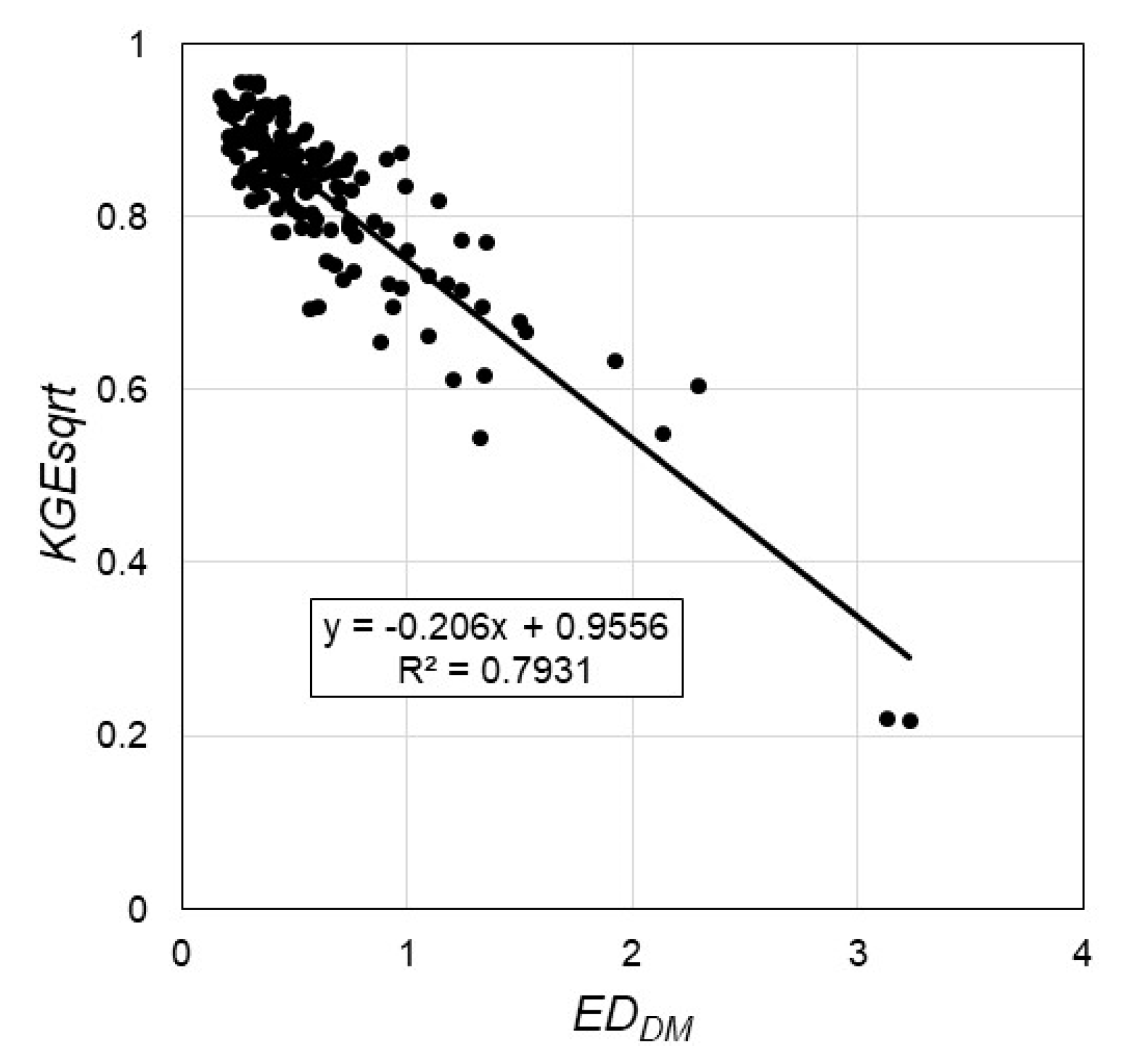
The $KGE$ and its variants are kinds of the Euclidian distance (ED) between the optimal and ideal points for correlation, bias, variance, and variability (Equations (10)–(15)). Pfannerstill et al. [71] proposed another form of the ED ($E{D}_{DM}$, Equation (17)) as an objective function. The two ED measures, $KGE$s and $E{D}_{DM}$, are similar to each other because both consider pairwise differences ($r$ and $NSE$), water balance ($\beta$ and $PBIAS$), and flow variability ($\alpha$, $\gamma$, $RSRQ0Q5$, $RSRQ5Q20$, and $RSRQ20Q70$):

$$E{D}_{DM}=\sqrt{\frac{1}{5}{\left(1-NSE\right)}^2+\frac{1}{5}\left(\frac{PBIAS}{100}\right)+\frac{1}{5}{\left(RSRQ0Q5\right)}^2+\frac{1}{5}{\left(RSRQ5Q20\right)}^2+\frac{1}{5}{\left(RSRQ20Q70\right)}^2},$$

(17)

where $RSRQ0Q5$, $RSRQ5Q20$, and $RSRQ20Q70$ are RMSE-observations standard deviation ratio ($RSR$) [64] for the FDC segments of 0% to 5%, 5% to 20%, and 20% to 70%, respectively. We found that the values of $E{D}_{DM}$ are highly correlated with those of $KG{E}_{sqrt}$ in the study dataset ($R^2=0.79$; Figure 9). Such a finding implies that the ED-based statistics including $KGE$s and $E{D}_{DM}$ could serve as an objective function to efficiently count for the multiple evaluation aspects in an RR model regionalization.

5. Summary and Conclusions

This study explored ways to accurately regionalize an RR model, i.e., the 3-Tank model, and evaluated the performance of models regionalized on the basis of the calibration results made with different objective functions. We also demonstrated the impacts of objective function selection on RR model regionalization. Results showed that there was no significant difference between the performance of $optRMSE$ and $optKG{E}_{sqrt}$ when predicting high flow and water balance. However, the $optRMSE$ provided poorer performance in reproducing low flow and FDC than $optKG{E}_{sqrt}$. The ${{regKGE}^{\prime }}_{sqrt}$ provided high flow modeling performance similar to that of the calibrated models ($optRMSE$ and $optKG{E}_{sqrt}$). In addition, ${{regKGE}^{\prime }}_{sqrt}$ was superior to the $regRMSE$ when predicting low flow, water balance, and FDC in the study watersheds. Such evaluation results suggested that ${{regKGE}^{\prime }}_{sqrt}$ can serve as an effective objective function when regionalizing a daily rainfall-runoff simulation model for ungauged watersheds in Korea. The regionalization methods proposed in this study should be applicable to other watersheds, even though the regression equations developed using the method might not be suitable for them.

References

- Sivapalan, M. Prediction in ungauged basins: A grand challenge for theoretical hydrology. Hydrol. Process. 2003, 17, 3163–3170. [Google Scholar] [CrossRef]
- Razavi, T.; Coulibaly, P. Streamflow prediction in ungauged basins: Review of regionalization methods. J. Hydrol. Eng. 2013, 18, 958–975. [Google Scholar] [CrossRef]
- Hrachowitz, M.; Savenije, H.H.G.; Blöschl, G.; McDonnell, J.J.; Sivapalan, M.; Pomeroy, J.W.; Arheimer, B.; Blume, T.; Clark, M.P.; Ehret, U.; et al. A decade of predictions in ungauged basins (PUB)—A review. Hydrol. Sci. J. 2013, 58, 1198–1255. [Google Scholar] [CrossRef]
- Amiri, B.J.; Fohrer, N.; Cullmann, J.; Hörmann, G.; Müller, F.; Adamowski, J. Regionalization of Tank model using landscape metrics of catchments. Water Resour. Manag. 2016, 30, 5065–5085. [Google Scholar] [CrossRef]
- Yang, X.; Magnusson, J.; Xu, C.-Y. Transferability of regionalization methods under changing climate. J. Hydrol. 2019, 568, 67–81. [Google Scholar] [CrossRef]
- Devia, G.K.; Ganasri, B.P.; Dwarakish, G.S. A review on hydrological models. Aquat. Procedia 2015, 4, 1001–1007. [Google Scholar] [CrossRef]
- Fenicia, F.; Kavetski, D.; Savenije, H.H.G. Elements of a flexible approach for conceptual hydrological modeling: 1. Motivation and theoretical development. Water Resour. Res. 2011, 47. [Google Scholar] [CrossRef]
- Song, J.-H.; Her, Y.; Park, J.; Kang, M.-S. Exploring parsimonious daily rainfall-runoff model structure using the hyperbolic tangent function and Tank model. J. Hydrol. 2019, 574, 574–587. [Google Scholar] [CrossRef]
- Song, J.-H.; Kang, M.S.; Song, I.; Jun, S.M. Water balance in irrigation reservoirs considering flood control and irrigation efficiency variation. J. Irrig. Drain. Eng. 2016, 142, 04016003. [Google Scholar] [CrossRef]
- Fenicia, F.; Kavetski, D.; Savenije, H.H.G.; Clark, M.P.; Schoups, G.; Pfister, L.; Freer, J. Catchment properties, function, and conceptual model representation: Is there a correspondence? Hydrol. Process. 2014, 28, 2451–2467. [Google Scholar] [CrossRef]
- Poncelet, C.; Merz, R.; Merz, B.; Parajka, J.; Oudin, L.; Andréassian, V.; Perrin, C. Process-based interpretation of conceptual hydrological model performance using a multinational catchment set. Water Resour. Res. 2017, 53, 7247–7268. [Google Scholar] [CrossRef] [Green Version]
- Van Esse, W.R.; Perrin, C.; Booij, M.J.; Augustijn, D.C.M.; Fenicia, F.; Kavetski, D.; Lobligeois, F. The influence of conceptual model structure on model performance: A comparative study for 237 French catchments. Hydrol. Earth Syst. Sci. 2013, 17, 4227–4239. [Google Scholar] [CrossRef]
- Kim, H.Y.; Park, S.W. Simulating daily inflow and release rates for irrigation reservoirs (1): Modeling inflow rates by a linear reservoir model. J. Korean Soc. Agric. Eng. 1988, 60, 13–24. [Google Scholar]
- Yokoo, Y.; Kazama, S. Numerical investigations on the relationships between watershed characteristics and water balance model parameters: Searching for universal relationships among regional relationships. Hydrol. Process. 2012, 26, 843–854. [Google Scholar] [CrossRef]
- Seibert, J. Regionalisation of parameters for a conceptual rainfall-runoff model. Agric. For. Meteorol. 1999, 98–99, 279–293. [Google Scholar] [CrossRef]
- Wagener, T.; Wheater, H.S. Parameter estimation and regionalization for continuous rainfall-runoff models including uncertainty. J. Hydrol. 2006, 320, 132–154. [Google Scholar] [CrossRef]
- Yokoo, Y.; Kazama, S.; Sawamoto, M.; Nishimura, H. Regionalization of lumped water balance model parameters based on multiple regression. J. Hydrol. 2001, 246, 209–222. [Google Scholar] [CrossRef]
- An, J.H.; Song, J.H.; Kang, M.S.; Song, I.; Jun, S.M.; Park, J. Regression equations for estimating the TANK model parameters. J. Korean Soc. Agric. Eng. 2015, 57, 121–133. [Google Scholar] [CrossRef]
- Kim, H.S. Adequacy of a multi-objective regional calibration method incorporating a sequential regionalisation. Water Resour. Manag. 2014, 28, 5507–5526. [Google Scholar] [CrossRef]
- Bastola, S.; Ishidaira, H.; Takeuchi, K. Regionalisation of hydrological model parameters under parameter uncertainty: A case study involving TOPMODEL and basins across the globe. J. Hydrol. 2008, 357, 188–206. [Google Scholar] [CrossRef]
- Prieto, C.; Vine, N.L.; Kavetski, D.; García, E.; Medina, R. Flow prediction in ungauged catchments using probabilistic random forests regionalization and new statistical adequacy tests. Water Resour. Res. 2019, 55, 4364–4392. [Google Scholar] [CrossRef]
- Rojas-Serna, C.; Lebecherel, L.; Perrin, C.; Andréassian, V.; Oudin, L. How should a rainfall-runoff model be parameterized in an almost ungauged catchment? A methodology tested on 609 catchments. Water Resour. Res. 2016, 52, 4765–4784. [Google Scholar] [CrossRef] [Green Version]
- Bulygina, N.; Ballard, C.; McIntyre, N.; O’Donnell, G.; Wheater, H. Integrating different types of information into hydrological model parameter estimation: Application to ungauged catchments and land use scenario analysis. Water Resour. Res. 2012, 48. [Google Scholar] [CrossRef] [Green Version]
- McIntyre, N.; Lee, H.; Wheater, H.; Young, A.; Wagener, T. Ensemble predictions of runoff in ungauged catchments. Water Resour. Res. 2005, 41. [Google Scholar] [CrossRef] [Green Version]
- Yang, C.; Wang, N.; Wang, S. A comparison of three predictor selection methods for statistical downscaling. Int. J. Climatol. 2017, 37, 1238–1249. [Google Scholar] [CrossRef]
- Zhang, Z.; Wagener, T.; Reed, P.; Bhushan, R. Reducing uncertainty in predictions in ungauged basins by combining hydrologic indices regionalization and multiobjective optimization. Water Resour. Res. 2008, 44, doi. [Google Scholar] [CrossRef]
- Beven, K.; Freer, J. Equifinality, data assimilation, and uncertainty estimation in mechanistic modelling of complex environmental systems using the GLUE methodology. J. Hydrol. 2001, 249, 11–29. [Google Scholar] [CrossRef]
- Merz, R.; Blöschl, G. Regionalisation of catchment model parameters. J. Hydrol. 2004, 287, 95–123. [Google Scholar] [CrossRef] [Green Version]
- Beven, K.; Binley, A. The future of distributed models: Model calibration and uncertainty prediction. Hydrol. Process. 1992, 6, 279–298. [Google Scholar] [CrossRef]
- Freer, J.; Beven, K.; Ambroise, B. Bayesian estimation of uncertainty in runoff prediction and the value of data: An application of the GLUE approach. Water Resour. Res. 1996, 32, 2161–2173. [Google Scholar] [CrossRef]
- Efstratiadis, A.; Koutsoyiannis, D. One decade of multi-objective calibration approaches in hydrological modelling: A review. Hydrol. Sci. J. 2010, 55, 58–78. [Google Scholar] [CrossRef]
- Her, Y.; Seong, C. Responses of hydrological model equifinality, uncertainty, and performance to multi-objective parameter calibration. J. Hydroinformatics 2018, 20, 864–885. [Google Scholar] [CrossRef] [Green Version]
- Kollat, J.B.; Reed, P.M.; Wagener, T. When are multiobjective calibration trade-offs in hydrologic models meaningful? Water Resour. Res. 2012, 48, doi. [Google Scholar] [CrossRef]
- Oudin, L.; Andréassian, V.; Mathevet, T.; Perrin, C.; Michel, C. Dynamic averaging of rainfall-runoff model simulations from complementary model parameterizations. Water Resour. Res. 2006, 42, doi. [Google Scholar] [CrossRef]
- Zhang, R.; Moreira, M.; Corte-Real, J. Multi-objective calibration of the physically based, spatially distributed SHETRAN hydrological model. J. Hydroinformatics 2016, 18, 428–445. [Google Scholar] [CrossRef]
- Song, J.-H.; Her, Y.; Park, J.; Lee, K.-D.; Kang, M.-S. Simulink implementation of a hydrologic model: A Tank model case study. Water 2017, 9, 639. [Google Scholar] [CrossRef]
- Sugawara, M. Automatic calibration of the tank model. Hydrol. Sci. Bull. 1979, 24, 375–388. [Google Scholar] [CrossRef]
- Chen, S.-K.; Chen, R.-S.; Yang, T.-Y. Application of a tank model to assess the flood-control function of a terraced paddy field. Hydrol. Sci. J. 2014, 59, 1020–1031. [Google Scholar] [CrossRef] [Green Version]
- Fumikazu, N.; Toshisuke, M.; Yoshio, H.; Hiroshi, T.; Kimihito, N. Evaluation of water resources by snow storage using water balance and tank model method in the Tedori River basin of Japan. Paddy Water Environ. 2013, 11, 113–121. [Google Scholar] [CrossRef]
- Huh, Y.M.; Park, S.W.; Im, S.J. A streamflow network model for daily water supply and demands on small watershed (1): Simulating daily streamflow from small watersheds. J. Korean Soc. Agric. Eng. 1993, 35, 40–49. [Google Scholar]
- Kim, S.J.; Kim, P.S.; Yoon, C.Y. A regression equation of Tank model parameters for daily runoff estimation in a region with insufficient hydrological data. In Proceedings of the 2010 KSAE Annual Conference; Journal of the Korean Society of Agricultural Engineers: Gyeonggi-do, Korea, 2000; pp. 412–418. [Google Scholar]
- Nash, J.E.; Sutcliffe, J.V. River flow forecasting through conceptual models part I—A discussion of principles. J. Hydrol. 1970, 10, 282–290. [Google Scholar] [CrossRef]
- Legates, D.R.; McCabe, G.J. Evaluating the use of “goodness-of-fit” Measures in hydrologic and hydroclimatic model validation. Water Resour. Res. 1999, 35, 233–241. [Google Scholar] [CrossRef]
- Pfannerstill, M.; Guse, B.; Fohrer, N. Smart low flow signature metrics for an improved overall performance evaluation of hydrological models. J. Hydrol. 2014, 510, 447–458. [Google Scholar] [CrossRef]
- Gupta, H.V.; Kling, H.; Yilmaz, K.K.; Martinez, G.F. Decomposition of the mean squared error and NSE performance criteria: Implications for improving hydrological modelling. J. Hydrol. 2009, 377, 80–91. [Google Scholar] [CrossRef] [Green Version]
- Kling, H.; Fuchs, M.; Paulin, M. Runoff conditions in the upper Danube basin under an ensemble of climate change scenarios. J. Hydrol. 2012, 424–425, 264–277. [Google Scholar] [CrossRef]
- Santos, L.; Thirel, G.; Perrin, C. Pitfalls in using log-transformed flows within the KGE criterion. Hydrol. Earth Syst. Sci. 2018, 22, 4583–4591. [Google Scholar] [CrossRef]
- Allen, R.G.; Pereira, L.S.; Raes, D.; Smith, M. Crop Evapotranspiration-Guidelines for Computing Crop Water Requirements; FAO—Food and Agriculture Organization of the United Nations: Rome, Italy, 1998; p. D05109. [Google Scholar]
- Kang, M.G.; Lee, J.H.; Park, K.W. Parameter regionalization of a Tank model for simulating runoffs from ungauged watersheds. J. Korea Water Resour. Assoc. 2013, 46, 519–530. [Google Scholar] [CrossRef]
- Duan, Q.; Sorooshian, S.; Gupta, V.K. Optimal use of the SCE-UA global optimization method for calibrating watershed models. J. Hydrol. 1994, 158, 265–284. [Google Scholar] [CrossRef]
- Gupta, H.V.; Sorooshian, S.; Yapo, P.O. Status of automatic calibration for hydrologic models: Comparison with multilevel expert calibration. J. Hydrol. Eng. 1999, 4, 135–143. [Google Scholar] [CrossRef]
- Her, Y.G. HYSTAR: Hydrology and Sediment Transport Simulation Using Time-Area Method. Ph.D. Thesis, Virginia Tech, Blacksburg, VA, USA, 2011. [Google Scholar]
- Duan, Q.; Sorooshian, S.; Gupta, V. Effective and efficient global optimization for conceptual rainfall-runoff models. Water Resour. Res. 1992, 28, 1015–1031. [Google Scholar] [CrossRef]
- Hrachowitz, M.; Fovet, O.; Ruiz, L.; Euser, T.; Gharari, S.; Nijzink, R.; Freer, J.; Savenije, H.H.G.; Gascuel-Odoux, C. Process consistency in models: The importance of system signatures, expert knowledge, and process complexity. Water Resour. Res. 2014, 50, 7445–7469. [Google Scholar] [CrossRef] [Green Version]
- Krause, P.; Boyle, D.P.; Bäse, F. Comparison of different efficiency criteria for hydrological model assessment. Adv. Geosci. 2005, 5, 89–97. [Google Scholar] [CrossRef] [Green Version]
- Crochemore, L.; Perrin, C.; Andréassian, V.; Ehret, U.; Seibert, S.P.; Grimaldi, S.; Gupta, H.; Paturel, J.-E. Comparing expert judgement and numerical criteria for hydrograph evaluation. Hydrol. Sci. J. 2015, 60, 402–423. [Google Scholar] [CrossRef]
- Moriasi, D.N.; Gitau, M.W.; Daggupati, P. Hydrologic and water quality models: Performance measures and evaluation criteria. Trans. ASABE 2015, 58, 1763–1785. [Google Scholar]
- James, G.; Witten, D.; Hastie, T.; Tibshirani, R. An Introduction to Statistical Learning; Springer: New York, NY, USA, 2013. [Google Scholar]
- Song, J.-H. Hydrologic Analysis System with Multi-Objective Optimization for Agricultural Watersheds. Ph.D. Thesis, Seoul National University, Seoul, Korea, 2017. [Google Scholar]
- Horton, R.E. Drainage-basin characteristics. Eos Trans. Am. Geophys. Union 1932, 13, 350–361. [Google Scholar] [CrossRef]
- Thiessen, A.H. Precipitation averages for large areas. Mon. Weather Rev. 1911, 39, 1082–1089. [Google Scholar] [CrossRef]
- Kang, M.S.; Park, S.W.; Lee, J.J.; Yoo, K.H. Applying SWAT for TMDL programs to a small watershed containing rice paddy fields. Agric. Water Manag. 2006, 79, 72–92. [Google Scholar] [CrossRef]
- Gan, T.Y.; Dlamini, E.M.; Biftu, G.F. Effects of model complexity and structure, data quality, and objective functions on hydrologic modeling. J. Hydrol. 1997, 192, 81–103. [Google Scholar] [CrossRef]
- Moriasi, D.N.; Arnold, J.G.; Van Liew, M.W.; Bingner, R.L.; Harmel, R.D.; Veith, T.L. Model evaluation guidelines for systematic quantification of accuracy in watershed simulations. Trans. ASABE 2007, 50, 885–900. [Google Scholar] [CrossRef]
- Tingsanchali, T.; Gautam, M.R. Application of Tank, NAM, ARMA and neural network models to flood forecasting. Hydrol. Process. 2000, 14, 2473–2487. [Google Scholar] [CrossRef]
- Black, P.E. Hydrograph responses to geomorphic model watershed characteristics and precipitation variables. J. Hydrol. 1972, 17, 309–329. [Google Scholar] [CrossRef]
- Lin, P.-S.; Lin, J.-Y.; Hung, J.-C.; Yang, M.-D. Assessing debris-flow hazard in a watershed in Taiwan. Eng. Geol. 2002, 66, 295–313. [Google Scholar] [CrossRef]
- Zhang, C.; Takase, K.; Oue, H.; Ebisu, N.; Yan, H. Effects of land use change on hydrological cycle from forest to upland field in a catchment, Japan. Front. Struct. Civ. Eng. 2013, 7, 456–465. [Google Scholar] [CrossRef]
- Clarke, R.T. A critique of present procedures used to compare performance of rainfall-runoff models. J. Hydrol. 2008, 352, 379–387. [Google Scholar] [CrossRef]
- Pushpalatha, R.; Perrin, C.; Moine, N.L.; Andréassian, V. A review of efficiency criteria suitable for evaluating low-flow simulations. J. Hydrol. 2012, 420–421, 171–182. [Google Scholar] [CrossRef]
- Pfannerstill, M.; Bieger, K.; Guse, B.; Bosch, D.D.; Fohrer, N.; Arnold, J.G. How to constrain multi-objective calibrations of the SWAT model using water balance components. J. Am. Water Resour. Assoc. 2017, 53, 532–546. [Google Scholar] [CrossRef]
Figure 2.
Spatial variations in the hydrologic characteristics of the 49 study watersheds.
Figure 3.
Comparison of performance statistics (, , , and ) provided by the 3-Tank models calibrated at the outlets of 39 study watersheds with two objective functions ( and ). The height of a box plot represents the interquartile range (IQR) (or the distance between the 75th and 25th percentiles), and the ends of whiskers signify the maximum and minimum values. Circles beyond the whisker ends are outliers.
Figure 4.
Comparison of the distributions of model parameter values calibrated using the objective functions of and .
Figure 5.
Correlation between calibrated parameter values and selected watershed characteristics. (a) and (b) . (*, **, and *** indicate , 0.01, and 0.001, respectively).
Figure 6.
Comparison of performance statistics (, , , and ) provided by the calibrated ( and ) and regionalized models ( and ) for the 39 study watersheds used for regionalization.
Figure 7.
Comparison of performance statistics (, , , and ) provided by the two regression models ( and ) for the 10 validation watersheds.
Figure 8.
Variation of performance statistics (, , , and ) provided by and other regional models for 10 verification watersheds.
Figure 9.
Scatterplot of vs. .