A Landscape Connectivity Approach for Determining Minimum Ecological Lake Level: Implications for Lake Restoration
by
Dan Liu
1,2, 
Xuan Wang
1,2,*,
Yun-long Zhang
1,2,
Sheng-jun Yan
1,2,
Bao-shan Cui
1,3 and
Zhi-feng Yang
1,2,3 1
State Key Laboratory of Water Environment Simulation, Beijing Normal University, Beijing 100875, China
2
Key Laboratory for Water and Sediment Sciences of Ministry of Education, Beijing Normal University, Beijing 100875, China
3
Beijing Engineering Research Center for Watershed Environmental Restoration and Integrated Ecological Regulation, Beijing Normal University, Beijing 100875, China
*
Author to whom correspondence should be addressed.
Water 2019, 11(11), 2237; https://doi.org/10.3390/w11112237
Submission received: 24 September 2019
/
Revised: 18 October 2019
/
Accepted: 21 October 2019
/
Published: 26 October 2019
(This article belongs to the Special Issue Techniques and Applications in Water Science and Engineering: Selected Papers from the Inaugural International Symposium on Water Modelling (iSymWater2019))
Abstract
:We proposed a new approach to determine the minimum ecological lake level using a landscape connectivity approach. Using MIKE 21 and ArcGIS software, we simulated the water landscape and corresponding connectivity of Baiyangdian Lake on the North China Plain and analyzed the relationship between landscape connectivity and lake level. The minimum ecological lake level was defined as the breakpoint of the lake level-connectivity curve. Results suggested that the minimum ecological lake level of Baiyangdian Lake is 7.8–8.0 m, below which lake ecosystems become fragmented and potentially fragile. Alternatively, better connectivity at lower lake levels may be achieved by engineered modification of landscape patterns. Such approaches can mitigate the waste of water and economic resources due to excessive reliance on increasing water levels to meet minimum connectivity requirements. This approach provided a new perspective for lake ecosystem restoration of use in water-resource- and landscape management.
1. Introduction
Affected by climate change and human activities, the accessibility of ecological lake water has seriously decreased, especially in arid areas [1,2]. Such a lack of accessibility results in lake degradation, followed by a decline in ecological services and functions with respect to water conservation, flood water storage, water purification, biodiversity protection and climate regulation [3]. Lake level is an important characteristic of the lake ecosystem [4]. Lake ecosystem functions are closely related to lake level, which influences habitat availability, complexity, and quality [5]. The minimum ecological lake level, a threshold below which the lake ecosystem will become severely depleted, is the key to determining the minimum ecological water demand of lake ecosystems [6]. Thus, the determination of minimum ecological lake levels has become an important factor in water resources allocation and lake restoration management.
In recent decades, several methods have been proposed to identify minimum ecological lake levels based on the relationship between lake levels and lake ecosystem characteristics. Such methods include the historical lake level method, lake morphology analysis, habitat analysis, species-environment models, water balance analysis, water quality modeling, and combinations of the above methods [6,7,8]. The first four of these techniques have been wildly used in practice, including applications at Nansi Lake, Dongting Lake, Honghe Lake, Bosten Lake, Baiyangdian Lake and Bakhtegan Lake [6,8,9,10]. These methods each take different philosophical and practical approaches. For example, the historical lake level method defines minimum ecological lake level as a statistic of the historical lake level records, while the lake morphology analysis defines the minimum ecological lake level as the inflection point of the lake level-area curve or the lake surface area-storage curve [4,6,8]. These methods take the lake as a whole without reflecting internal structures of lakes and their related differences in ecological services of lake sub-regions. Actually, the spatial heterogeneity of connectivity for lake sub-regions usually has important impacts on the material and energy transfer of the ecosystem, and it will affect the evolution of the ecosystem in the long term [11]. In recent years, the development of landscape ecology has brought new perspectives for the study of impacts of spatial relations among lake sub-regions on ecosystem functions [12]. However, these methods have yet to take on a landscape perspective so far, which can provide a more rational and effective conceptual framework for solving practical environmental and ecological problems with respect to temporal and spatial heterogeneity [13].
Connectivity is a vital element of landscape structure, and has become a focus of modern ecosystem management [14,15]. Landscape connectivity is widely defined as “the degree to which a landscape facilitates or impedes movement among resource patches” [16]. In general, different water levels within shallow lakes result in different water landscape patterns and corresponding connectivity. Connectivity of water landscapes determines the potential connectivity of hydrology. In turn, alterations in hydrological connectivity induce changes in connectivity with respect to materials, energy, and aquatic organisms, subsequently contributing to the evolution of lake ecosystems [17,18,19]. In general, poor connectivity usually results in the disruption of internal energy flows and nutrient cycles, and often leads to degradation of the lake ecosystem [20]. Thus, connectivity is an important indicator of the lake ecosystem health and the maintenance of minimum connectivity is essential for preventing degradation. Based on the relationship between lake connectivity and lake level, the minimum ecological lake level corresponding to the minimum lake connectivity necessary to maintain lake ecosystems can be determined, thus providing a decision-making basis for lake ecosystem regulation and management.
This study proposes a landscape connectivity approach for determining the minimum ecological lake level by analyzing the relationship between lake level and connectivity. This approach was used to determine the minimum ecological lake level of a typical shallow lake, Baiyangdian Lake on the North China Plain. In contrast to traditional methods, which take the perspectives of hydrology, hydraulics or ecology, this is the first discussion of minimum ecological lake level from a landscape perspective. The landscape connectivity approach provides a new perspective on the problem of lake restoration by regulating landscape patterns with respect to the transfer efficiency of matter, energy, and organisms within lakes. Results of this study can not only give guidance in support of water resource allocation, but also direct engineering solutions based on landscape pattern planning. Optimization of landscape patterns provides an alternative to water diversion as a means to improve connectivity, to ensure that ecological water requirements are met and to prevent lake degradation as a result of water shortages.
2. Study Area
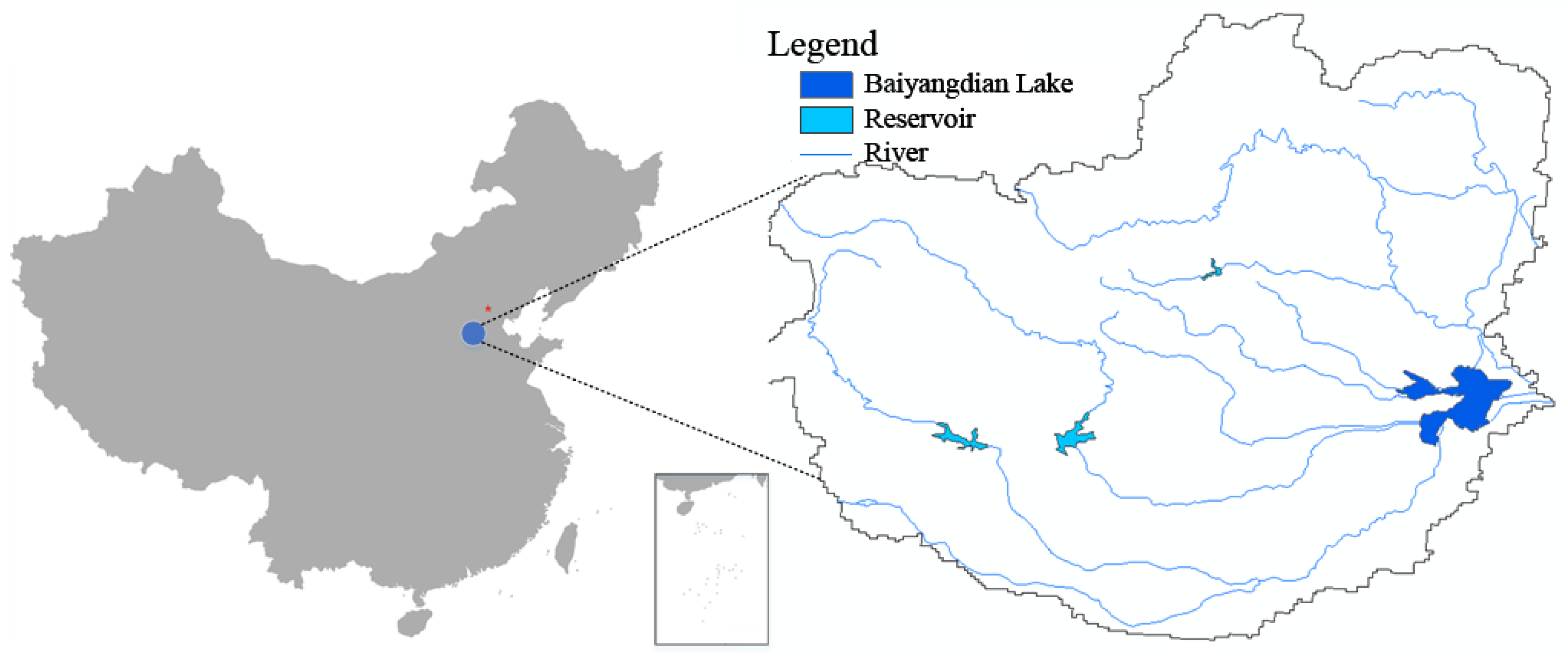
Baiyangdian Lake (38°43′ N–39°02′ N, 115°38′–116°07′ E) is located in the middle of the North China Plain (Figure 1). It is the largest remaining freshwater lake in northern China, as well as one of the most important water areas in the Xiong’an new area, a newly developed center for government functions and employees relocated from Beijing. The lake consists of 143 sub lakes and more than 3700 channels, covering an area of 366 km2, with an elevation ranging from 5.5 to 6.5 m [21]. Inflow is sourced from nine rivers within the larger Daqing River Basin, giving Baiyangdian Lake an important role in regional flood control and irrigation water storage. Outflow is discharged to Zhaowang New River, controlled by Zaolinzhuang brake, which would be opened when the water level exceeds 10.5 m during the high flows.
Owing to a semiarid temperate continental monsoon climate, Baiyangdian Lake receives an average annual precipitation of 550 mm, mostly in the summer (70–80%), and has an average annual temperature of 7–12 °C [22]. Water loss due to evaporation and seepage is high. Annual average evaporation is 1366 mm and seepage from the lake is about 2 × 10⁸ m3 [23]. Meanwhile, more than 150 reservoirs have been built upstream of the lake since 1958 [24]. As a result, streamflow into the lake has dramatically decreased, leading to decreased average annual lake levels (Figure 2) and increased frequency of drying up. Baiyangdian Lake only dried up once during the period 1919–1965, but has dried up frequently during the period 1965–2002 [25]. Such drying has caused serious environmental and ecological problems including area shrinkage, water pollution and a decline in biological resources [9,23]. The government of China has made great efforts to restore Baiyangdian Lake. For example, a nature reserve established in November 2002 contains four kinds of birds under first-class state protection and 26 kinds of birds under second-class state protection. Additionally, water diversion projects have been conducted at both the basin-level and inter-basin scale for meeting the ecological water requirements of Baiyangdian Lake. Examples include the “Water Diversion from the Yellow River to Lake Baiyangdian” project and the “South-to-North Water Diversion” project [23]. However, because the minimum ecological lake level remains unclear, it is not yet possible to provide optimized proper guidance for water resource management and lake restoration.
Baiyangdian Lake is a typical shallow lake. Accordingly, changes in lake level lead to dramatic changes in landscape patterns and connectivity. From 1990 to 2015, the overall connectivity of Baiyangdian lake was poor, first decreasing from 1990 to 2005 and then gradually recovering from 2005 to 2015 [20]. Ignoring hysteresis, this observation was consistent with the change law of the lake level. Due to the relative strong relationship between lake level and lake connectivity, Baiyangdian Lake is an appropriate area for studying the minimum ecological water level using a landscape connectivity approach.
3. Methods
3.1. Framework for Developing a Landscape Connectivity Approach to Determine the Minimum Ecological Lake Level
Lake level influences the area of water patches, which is an important factor in determining landscape connectivity. Therefore, we assumed that a direct relationship existed between lake level and connectivity. Ideally, the minimum ecological lake level will correspond to the minimum connectivity necessary to prevent lake degradation. The relationship between connectivity and lake level can be expressed by the following:
where C is the connectivity of water patches, and H is the lake level.
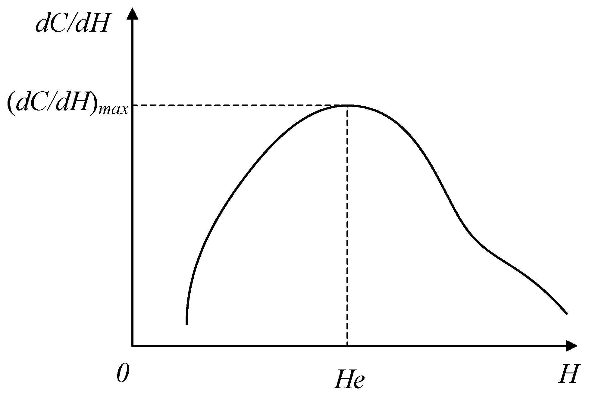
Generally, connectivity increases with the increased lake level. However, the rate of increasing connectivity as a function of lake level (dC/dH) may increase or decrease with the lake level. Similar to widely used lake morphology analysis methods [26], the minimum ecological lake level, He, can be determined as the critical lake level corresponding to the maximum dC/dH, that is
The connectivity corresponding to minimum ecological lake level is called the minimum ecological landscape connectivity. Accordingly, we define this approach as the landscape connectivity approach, as shown in Figure 3.
At the minimum ecological lake level, landscape connectivity is most sensitive to changes in lake level. A small drop in lake level would lead to a significant reduction in connectivity and a correspondingly significant degradation of lake ecosystems. Conversely, a small increase in lake level can provide a significant increase in connectivity and ecosystem health.
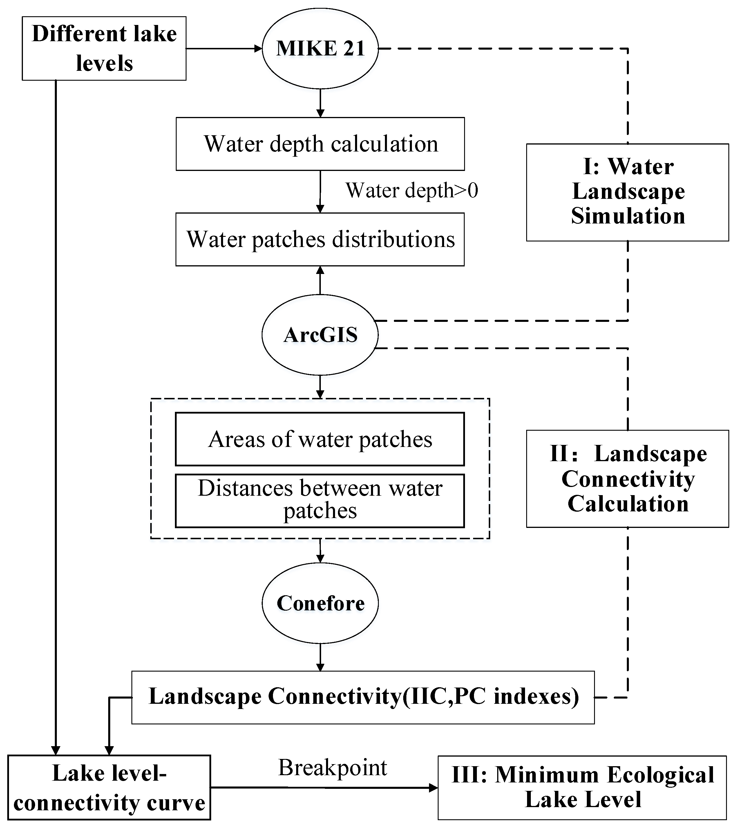
Three steps (Figure 4) are required to obtain the minimum ecological lake level:
- (1)
- Simulating landscape patterns of water at different lake levels. In this study, the hydrodynamic module (HD) of MIKE21 software was used to calculate the water depth at different lake levels based on measured topographic and bathymetric data of Baiyangdian Lake. Those grids with water depth greater than 0 m were then identified using ArcGIS and the distribution of water patches was mapped. It is also feasible to obtain the landscape patterns by interpreting Landsat images corresponding to known historical lake levels. However, Landsat images corresponding to different lake levels are not always available.
- (2)
- Calculating the connectivity of water patches. With ArcGIS, water patch areas and edge-to-edge Euclidean distances between patches were calculated. Connectivity was then calculated using CONEFOR software. Commonly used connectivity indexes include the integral index of connectivity (IIC) and the probability index of connectivity (PC).
- (3)
- Determining the minimum ecological lake level. Based on the relationship between connectivity and lake level, the lake level-connectivity (H-C) curve can be obtained. The breakpoint corresponding to the maximum dC/dH can then be determined and identified as the minimum ecological lake level of Baiyangdian Lake.
3.2. Water Landscape Simulation
As is typical of shallow lakes, the water landscape of Baiyangdian Lake is significantly influenced by lake level. Water landscape characteristics including water area and water spatial distributions were usually obtained by remote sensing. However, image interpretation in this case was significantly impeded by weather conditions, vegetation growth and other factors. In this study, the MIKE21 software, a useful tool with multiple modules such as hydrodynamics (HD), water quality and Ecolab modules for simulating the environment and ecology of wetlands, was used to simulate the water landscapes of Baiyangdian Lake under different lake level conditions.
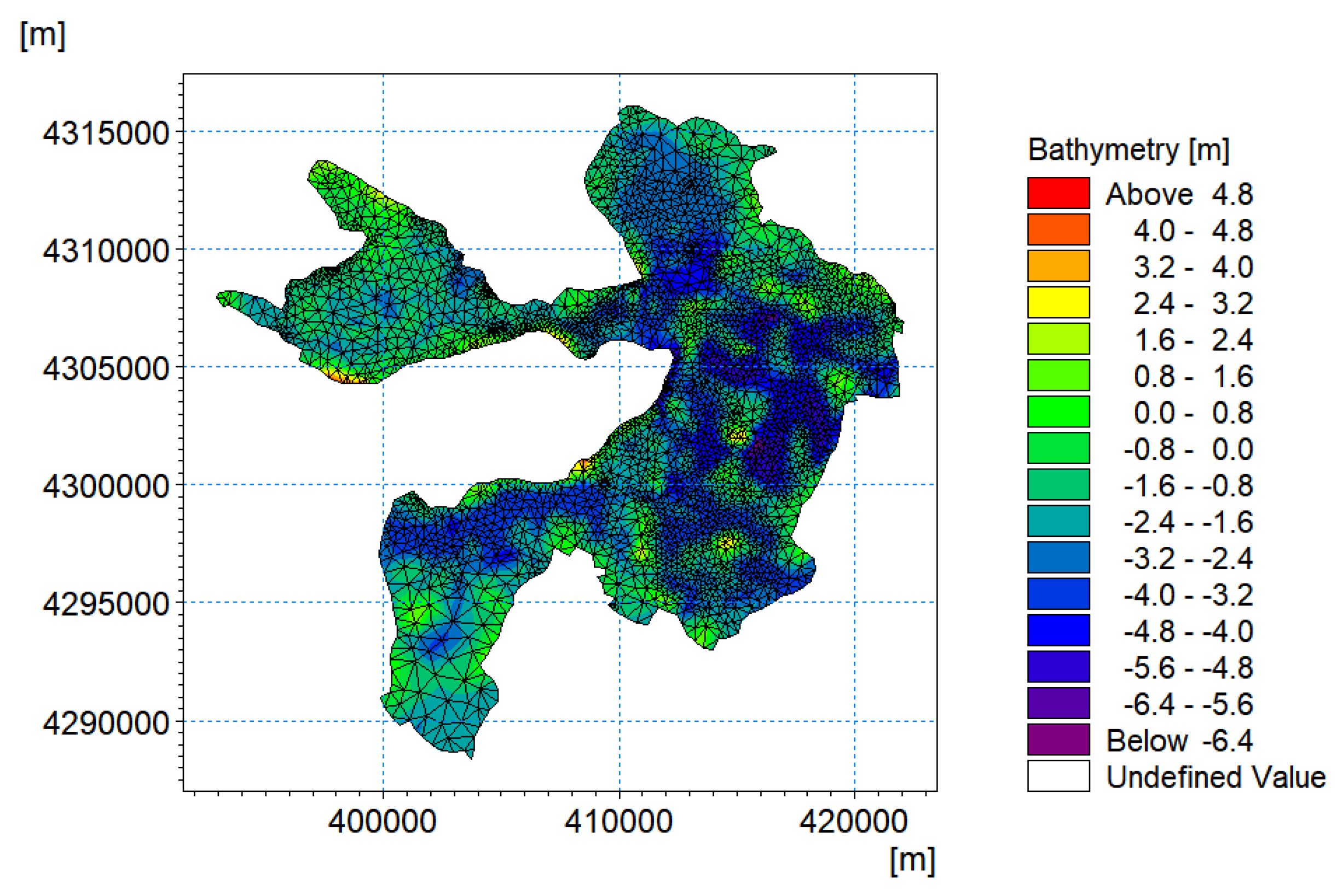
Using the HD module of MIKE21 software, the mesh generation, terrain interpolation, initial conditions and boundary conditions were required for water landscape simulation. First, the Mesh Generator of MIKE Zero was used to divide terrain grids using the triangular grid method. Based on the topographic characteristics of Baiyangdian Lake, the low-lying channels and the main watery areas were treated with mesh encryption. In total, 3460 grid cells were used. Following mesh generation, existing elevation data were used for terrain interpolation and to endue each grid node with an elevation attribute, as shown in Figure 5.
The initial conditions for solving HD included surface elevation and the initial velocity in the horizontal and vertical directions. Because there were a few spatial differences in lake level, the initial lake level at varied grid cells was set to be identical, that is, . The initial velocities in both the horizontal and vertical directions were set to zero. To keep the lake level stable, the boundary condition was set as land boundary (zero velocity), and rainfall and evaporation were set to zero. The solution parameters values were as shown in Table 1. By running the model with different initial lake levels, the distributions of water depth under varied lake levels in Baiyangdian Lake can be obtained.
3.3. Landscape Connectivity
In this study, two kinds of indices were adopted to reflect the landscape connectivity of Baiyangdian Lake, namely, the integral index of connectivity and the probability index of connectivity. These two indices can be calculated using the CONEFOR software package, which calculates a variety of graph-theoretic connectivity indices. Connectivity indices are calculated using the following functions:
- (1)
- Integral index of connectivity (IIC)where n represents the total number of water patches in the lake landscape, ai(or aj) is the area of an individual patch i (or j), nlij is the number of links in the shortest path between patch i and j, AL is the total area of the lake including water patches and non-water patches. In this approach, there are only two cases of connection and non-connection between two patches. Patches are judged to be connected or not based on the preset distance threshold value. If the distance between two patches is less than the threshold distance, the patches are connected; otherwise, patches are non-connected. The range of IIC is from zero to one, where zero indicates complete isolation between patches and one indicates that the whole lake is completely connected.
- (2)
- Probability index of connectivity (PC)where n, ai, aj and AL have the same meaning as that in Equation (3); is the maximum product probability of dispersal between patches i and j; dij is Euclidean edge to edge distance; k is a constant used to fit the function to user specified relationship between distance and dispersal probability. As with the IIC, the higher the PC value, the better the connectivity of the lake.
4. Results
4.1. Verification of Water Landscape Simulation
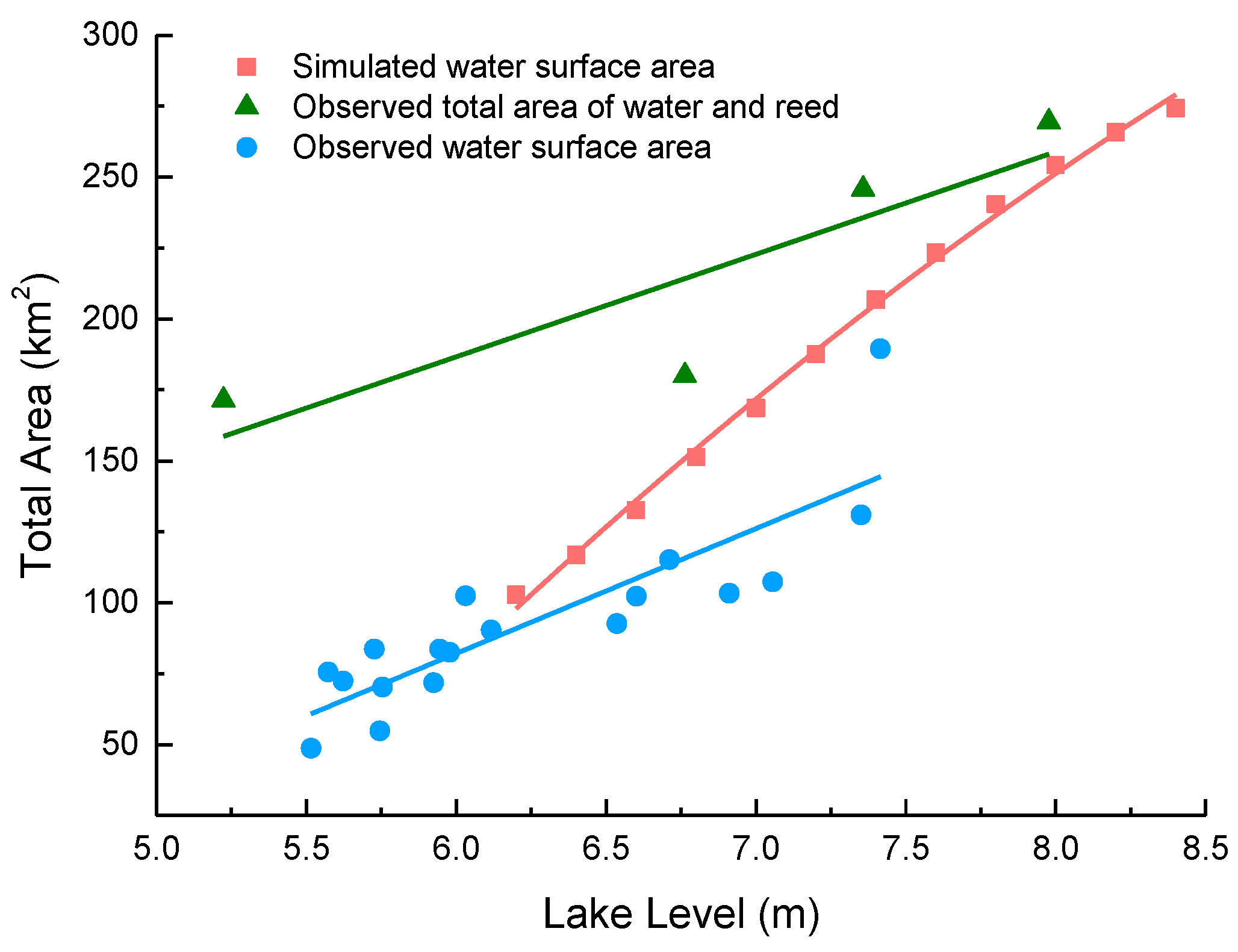
The water landscape was simulated using MIKE21 software and the water surface areas under different lake levels were then calculated using ArcGIS software. The water surface area was an important index of the landscape pattern and a key element for determining landscape connectivity. To verify the validity of the water landscape simulation, the lake level-water surface area curve obtained by numerical simulation was compared with that obtained by interpretation of historical satellite images. As shown in Figure 6, the observed water surface area under different lake level scenarios were obtained from Zhang et al. [27], while the observed total area of water and reeds under different lake levels were obtained from Zhuang et al. [22]. Results showed that water surface areas obtained from simulation were close to those obtained from image interpretation at low lake levels, when reed areas were not flooded by water. In contrast, at relatively high lake levels, reed areas were almost entirely flooded by water, so that the water surface areas obtained from simulation were close to the total area of water and reeds resolved from remote sensing images. The rational results demonstrated the validity of calculating water surface areas using MIKE21 software. Meanwhile, this simulation method can make up for the shortcomings of the remote sensing method in that remote sensing cannot accurately identify the extent of water surfaces when covered by reeds.
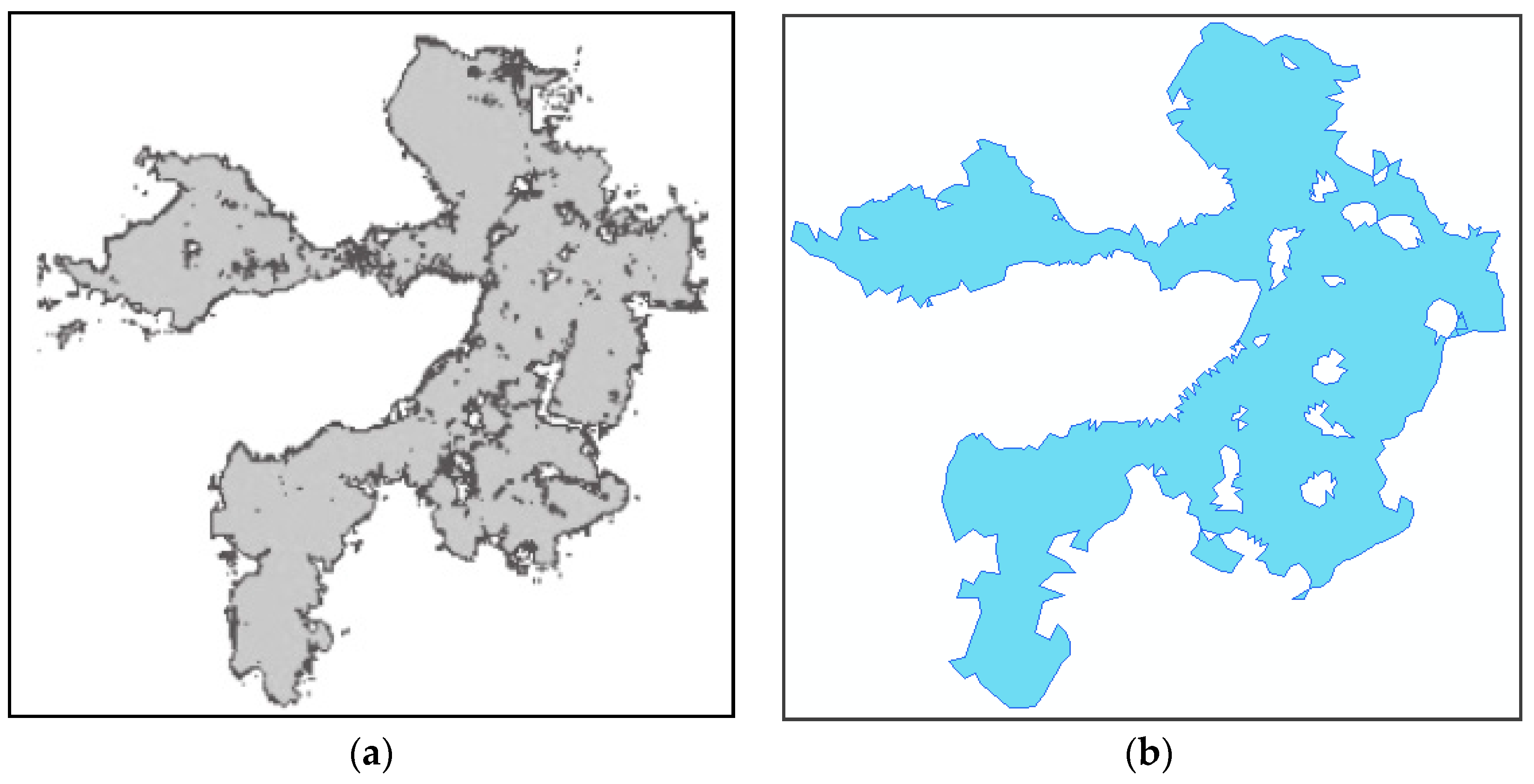
As an additional form of verification, the spatial distribution of water patches obtained from MIKE21 was mapped and compared with that obtained from remote sensing images. Figure 7a was the interpreted remote sensing image obtained from Zhang et al. [27] to display the distribution of water patches in February 1996 when less affected by reeds. The corresponding water surface area was 258 km2. Figure 7b mapped the water patches distribution with simulation at a lake level of 8.0 m, and the corresponding water surface area was 254.3 km2. Although some complex and small-area channels and reed lands were not identified, the spatial distribution of water patches obtained by numerical simulation was generally consistent with that obtained from remote sensing, indicating the reliability of the landscape simulation method. To obtain more precise results, additional topographic surveying and mapping were required to obtain a more accurate topographic map of the area.
4.2. Water Landscape Patterns under Different Lake Levels
According to previous studies that used more traditional methods including historical lake level method, lake morphology analysis and water balance analysis [28,29,30], the minimum ecological lake level of Baiyangdian Lake was in the range 7.02–7.76 m. Therefore, we selected lake levels from 6.2 m to 8.4 m to cover that range, and simulated the corresponding landscape patterns of water.
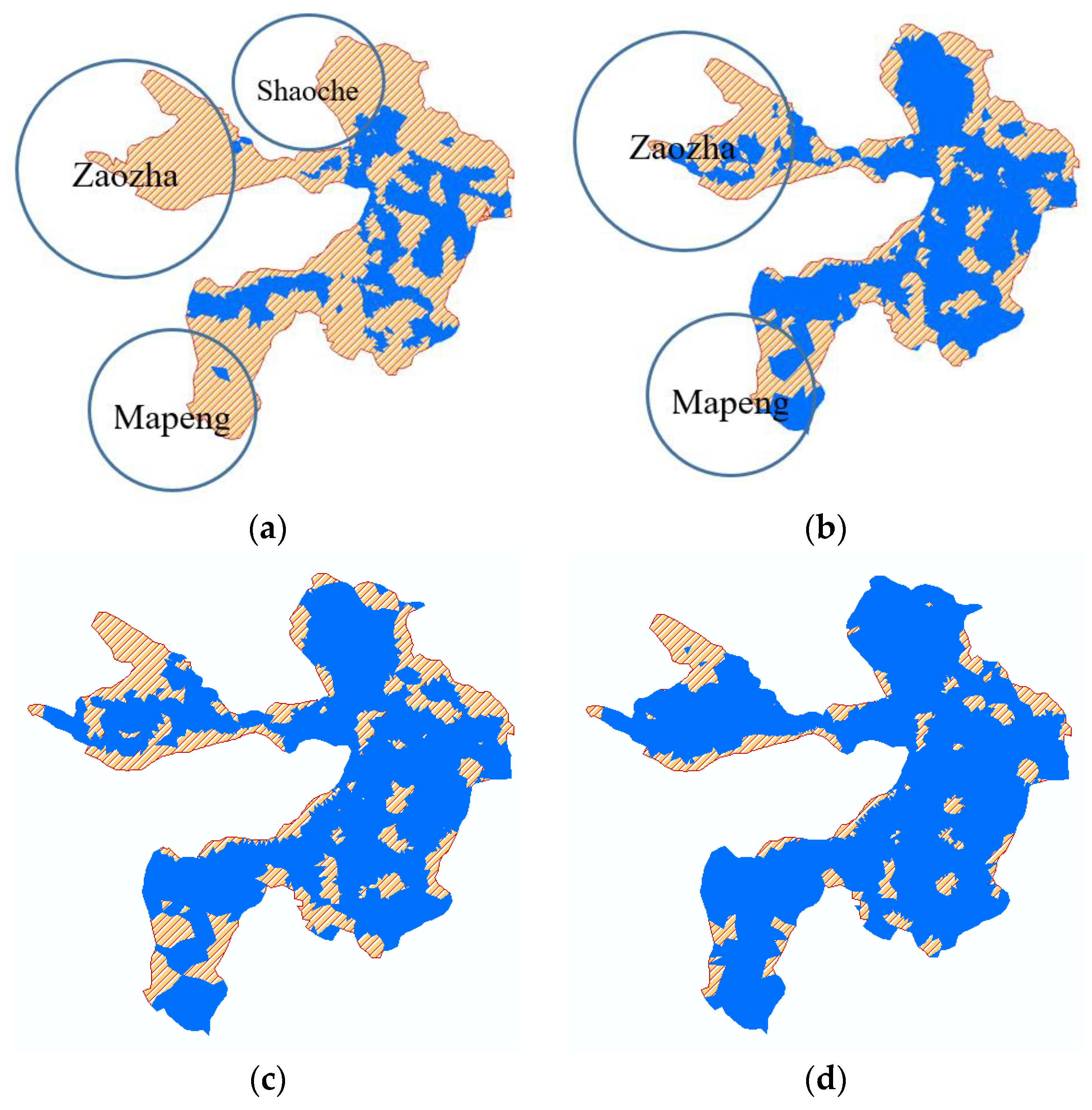
Some of the maps of landscape patterns for different lake levels derived from simulation are shown in Figure 8. It can be seen that under certain lake levels, Baiyangdian Lake actually consisted of many sub lakes. In particular, large areas of high ground were exposed at low lake levels, leading to many water patches being disconnected from each other. With the rise of lake levels, many reed lands were flooded and the area of the water patches increased. Meanwhile, the number of isolated patches decreased and almost no isolated water patches existing when the lake level was 8.4 m, indicating overall increased connectivity. Conversely, a drop-in lake level would lead to a significant reduction in connectivity. Results of connectivity calculations demonstrated that the integral index of connectivity (IIC) and probability index of connectivity (PC) decreased by 95.9% and 93.4% respectively, when the lake level decreased from 8.4 m to 6.2 m. Therefore, it is necessary and important to determine the minimum ecological lake level and to ascertain the minimum connectivity needed to maintain the ecosystem functions of Baiyangdian Lake.
In addition, according to Figure 8, connectivity of water landscape exhibited significant spatial heterogeneity, especially at low lake levels. For example, at a lake level of 6.2 m, the connectivity of Zaozha, Shaoche and Mapeng sub-lakes were much lower than those of other regions. With increased lake level, the spatial difference in connectivity gradually decreased, and the connectivity of the lake as a whole was high when the lake level increased to 8.4 m. Therefore, determination of the minimum ecological lake level should take into account the minimum connectivity of all or most sub lakes to prevent overall or partial degradation of the lakes.
4.3. Response of Landscape Connectivity to Lake Level Variations
The landscape connectivity expressed by IIC and PC were obtained using CONEFOR software. To determine the minimum ecological lake level, the first-order difference of IIC and PC were calculated and the gradient of connectivity over lake level (dC/dH) was estimated for each 0.2 m increase in lake level. The fitted curve of dC/dH and lake level (H) was obtained, as shown in Figure 9.
With decreasing lake level, dC/dH as determined by both IIC and PC first increased and then decreased. Thus, there was an identifiable breakpoint corresponding to the maximum dC/dH at which small differences in lake level correspond to relatively large differences in connectivity. The breakpoints of the IIC and PC curves occurred when lake level was 8.0 m and 7.8 m, respectively. That is to say, the IIC would be reduced most if the lake level decreased from 8.0 m to 7.8 m, while the PC would be reduced most if the lake level decreased from 7.8 m to 7.6 m. Such decreases in lake level would lead to a decrease of IIC by 29.0% (from 0.401 to 0.285) and a decrease of PC by 22.3% (from 0.403 to 0.342). To prevent lake degradation caused by sharp declines in connectivity, the minimum ecological lake level is recommended to be between 7.8 m and 8.0 m; the corresponding IIC at these lake levels were 0.28 and 0.34, respectively, and the corresponding PC were 0.34 and 0.4, respectively.
5. Discussion
5.1. Comparison of the Landscape Connectivity Approach with the Lake Morphology Approach
To verify the effectiveness of applying the landscape connectivity approach, results were additionally compared with those obtained using the lake morphology approach. Lake morphology analysis is one of the most commonly used methods for determining the minimum ecological lake level. It usually takes the water surface area, an important element for habitat protection, as a representative index for lake ecosystems. Accordingly, it defines minimum ecological lake level as the breakpoint of the lake level-area curve [26].
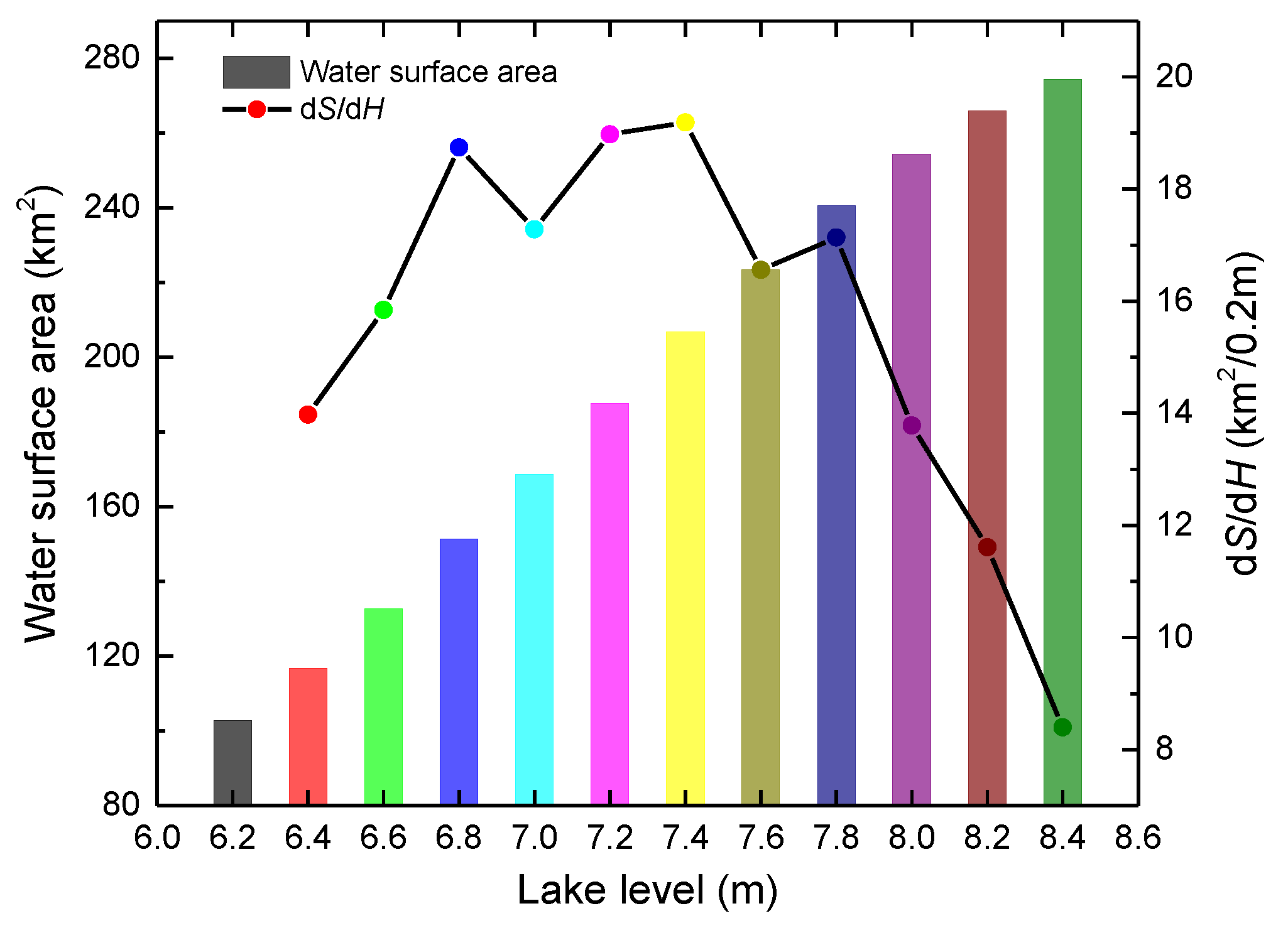
The results of lake morphology analysis are shown in Figure 10, where S is the water surface area, H is the lake level, and dS/dH represents the increased rate of water surface area with increased lake level. According to Figure 10, water surface area increased with increasing lake level, but the rate of increase varied. The rate of increased water surface area was relatively small when the lake level was less than 6.8 m or higher than 7.8 m. On the contrary, a small increase or decrease in lake level between 6.8 m and 7.8 m would induce a significant change in water surface area, with the rate achieving a maximum when the lake level was 7.4 m. Therefore, the minimum ecological lake level of Baiyangdian lake obtained by the lake morphology approach was 7.4 m, which was close to the result obtained by Zhao et al. [28].
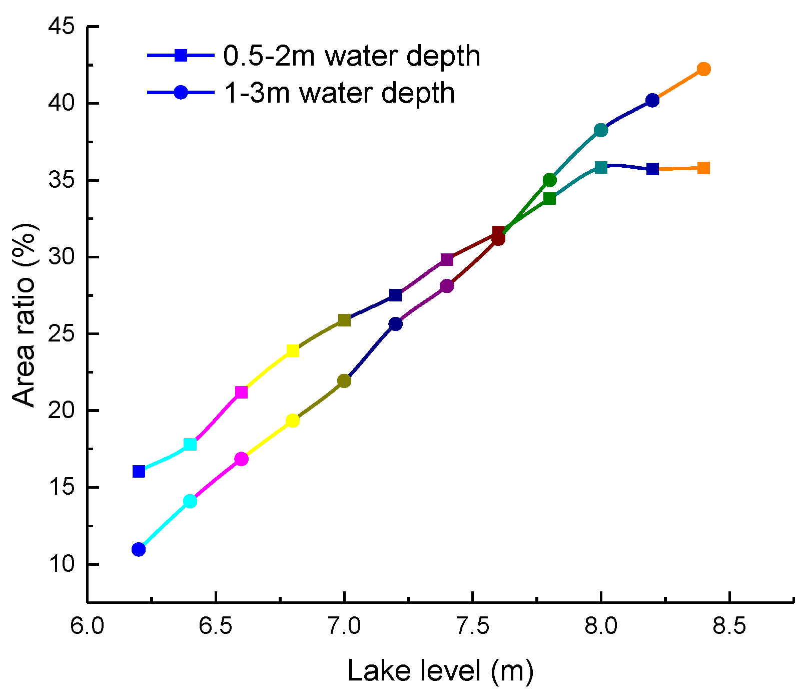
As the largest freshwater lake on the North China Plain, Baiyangdian Lake performs several ecosystem functions including flood water storage, water quality purification, biodiversity protection and landscape construction. Each of these functions has different requirements for water depth. Previous studies [29] have shown that 0.5–2 m water depth coverage is most conducive to the growth of aquatic vegetation such as reeds and lotus root, and at the same time reserves suitable habitat for fish spawning. Alternatively, a water depth of 1–3 m is most appropriate for landscape construction in surrounding cities.
As discussed in Section 4.3, the minimum ecological lake level obtained by the lake connectivity approach was between 7.8 m and 8.0 m, differing from that obtained by the traditional lake morphology approach. To compare the ecosystem functions of Baiyangdian Lake under the two different minimum ecological lake levels, the distribution of water depth under different lake levels were further analyzed. As shown in Figure 11, with the rise of lake level, the proportions of area with 0.5–2 m water depth and 1–3 m water depth both exhibited an increase at higher lake levels. When the lake level was less than 7.6 m, the proportion of area with 0.5–2 m water depth was higher than that with 1–3 m water depth, and vice versa when the lake level was higher than 7.6 m. That is to say, at the lake level of 7.4 m, the areas suitable for vegetation growth and fish spawning accounted for a higher proportion (29.8%) than that suitable for landscape construction (28.1%); while at 7.8 m the areas suitable for landscape construction accounted for a higher proportion (35.0%) than that suitable for vegetation growth and fish spawning (33.8%). Therefore, it can be concluded that following the recommendations obtained by the lake morphology method would lead to a situation more focused toward vegetation growth and fish spawning, while following the recommendations obtained by the lake connectivity method would lead to a situation more suited to landscape construction.
Because it was realized by a comprehensive analysis of the relationship between lake level-area and area-connectivity, the landscape connectivity approach can also be interpreted as a “lake level-area-connectivity approach”. The difference lay in that the connectivity method took into account the spatial distribution of water patches in addition to their total area. That is to say, although water surface area can be guaranteed under certain lake level conditions, the lack of connectivity between water patches may also lead to ecological degradation caused by poor energy flows and nutrient cycles and limited organisms migration. This may lead to a higher required minimum ecological lake level in shallow lakes (e.g., Baiyangdian Lake), which were strongly affected by human activities and exhibited high landscape fragmentation impeding connectivity between water patches. Compared with the lake morphology approach, which focused on the total habitat extent as measured by the water surface area, the landscape connectivity approach might be more suitable for shallow lakes, focusing on landscape connectivity with respect to internal transfer efficiencies of materials, energy and organisms within lakes. Through adjusting the landscape connectivity and thus controlling the transfer pathways and efficiencies for improving certain ecological functions, the landscape connectivity approach can provide a new theoretical basis for restoring lakes at the landscape scale.
5.2. Lake Restoration Recommendations Based on the Landscape Connectivity Approach
In the past, to meet the minimum ecological lake level, lake managers often focused on water transfer, typically ignoring the site-specific nature of the minimum ecological lake level, which was different under varied landscape patterns. This suggests that we can try to lower the minimum ecological lake level by optimizing the landscape patterns of the lake to prevent lake degradation without changing the lake level, which is an important consideration when water resources are extremely scarce. This recognition of the landscape-dependent nature of the minimum ecological lake level has especially important implication for lakes in arid regions, and the landscape connectivity approach makes this idea possible.
Taking Baiyangdian Lake as an example, it was possible to slightly reconstruct the landscape pattern to maintain better connectivity and potentially reduce the minimum ecological lake level. Based on the analyses presented in Section 4.3 and Section 5.1, it was clear that a lake level of 7.4 m can successfully meet the minimum ecological demand for surface area but cannot meet the minimum ecological demand for connectivity. Based on the lake level-storage curve measured by the Daqinghe River Affairs Department, raising the lake level to 7.8 m to ensure minimum connectivity required an additional 1.29 × 10³ m3 of water, even if losses through evaporation and leakage were ignored. In a dry year, it may not be possible to supply this amount of water from upstream reservoirs which also supplied urban industrial, agricultural and domestic water. However, water transferred through the “Water Diversion from the Yellow River to Lake Baiyangdian” project or the “South-to-North Water Diversion” project would lead to excess waste of both water and financial resources. In this context we explored an alternative plan, namely to enhance connectivity between different regions through local engineered restructuring of the landscape pattern.
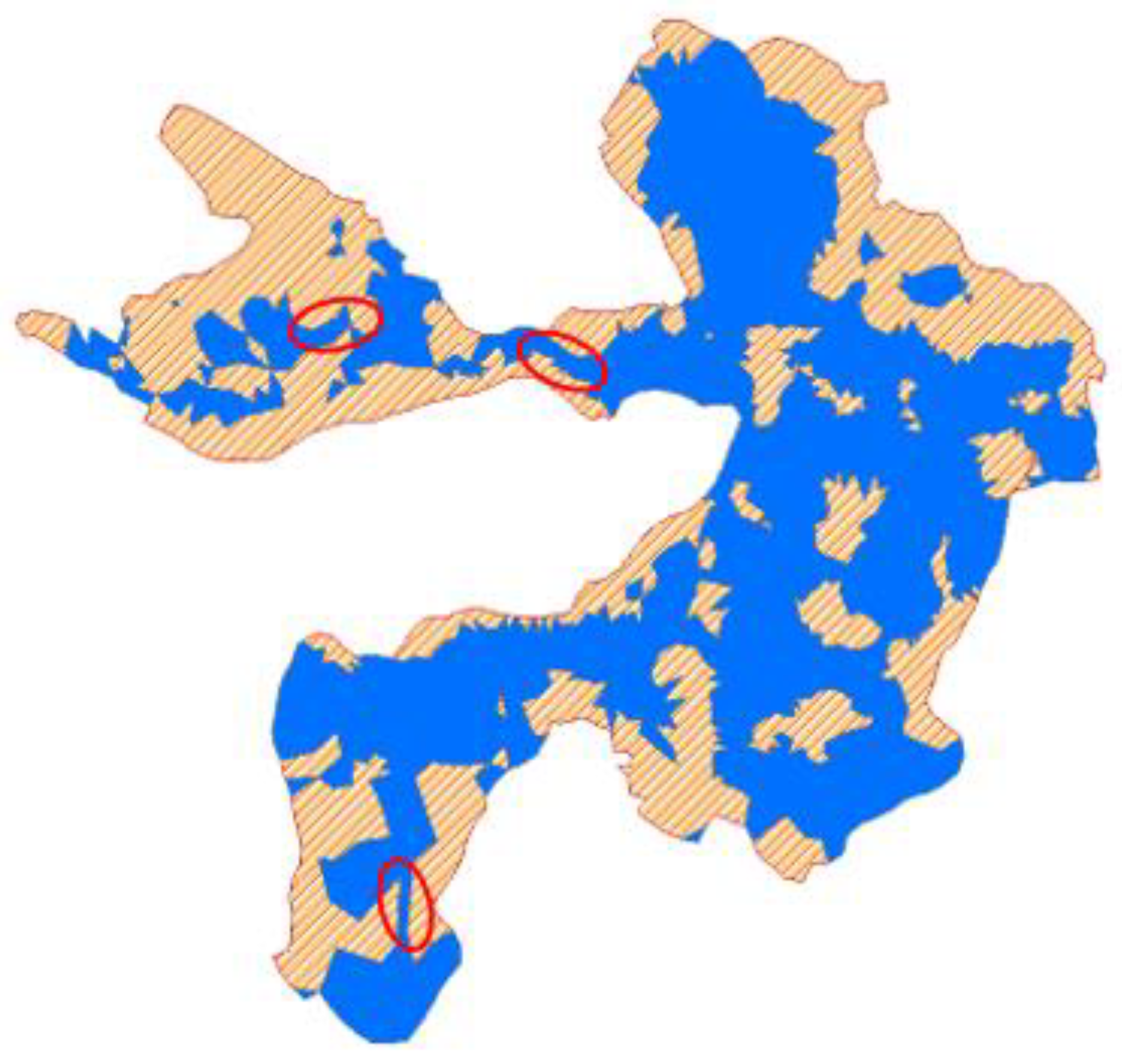
As shown in Figure 8, the sub lakes of Zaozha and Mapeng exhibited weak connectivity when the lake level was 7.4 m. Thus, it may be helpful to deepen the channel connecting neighbored sub-lakes or create a new trench as in Figure 12. Results showed that slight modifications to the landscape significantly increased both IIC and PC at a rate of 43% and 45%, respectively. Specifically, IIC increased from 0.18 to 0.26, while PC increased from 0.2 to 0.29. These values were much closer to the connectivity supported by the lake level of 7.8 m within the original landscape pattern. Thus, engineered modification of the landscape is able to improve connectivity and meet the minimum connectivity demand of the lake ecosystem at a low lake level of 7.4 m. The landscape connectivity approach can provide an effective pathway for restoring lakes by regulating landscape patterns in lake research and management.
6. Conclusions
By taking the water landscape connectivity as a critical ecosystem index, this research proposed a landscape connectivity approach to determine the minimum ecological lake level through identifying the breakpoint of the lake level-connectivity (H-C) curve. It was the first to determine the minimum ecological lake level from the perspective of landscape connectivity. Compared with traditional lake morphology approaches, which focused on overall habitat protection, the landscape connectivity approach focused more on the spatial distribution of water resources with respect to internal transfer efficiencies of materials, energy and organisms within lake ecosystems. This study also demonstrated that lake levels that met the requirement of minimum habitat area may not satisfy the minimum connectivity requirement of lake ecosystems. In this case, raising the water level to meet the minimum connectivity requirement only by water diversion would lead to a likely waste of both water and financial resources. Alternatively, landscape connectivity can be enhanced through local reconstruction of landscape patterns. Thus, better connectivity can be achieved at lower water levels. This discovery can provide a new approach for lake restoration through landscape connectivity management at relatively low economic costs.
This study developed a landscape connectivity approach based on the relationship between water level and lake connectivity from the perspective of landscape ecology, which can be further improved in future studies. For example, landscape connectivity is limited to reflect the potential connectivity of flows and nutrients, and some functional connectivity indices representing actual process of connectivity should be developed to replace landscape connectivity. Through further discussion of the relationship between lake level and functional connectivity, a more realistic minimum ecological lake level may be obtained. In addition, quantitative spatial differences in connectivity should be investigated to identify areas of weak connectivity, which usually are most sensitive to changes in lake level, thus providing more specific suggestions for managers.
Author Contributions
Conceptualization, D.L. and X.W.; methodology, D.L. and Y.-l.Z.; software, D.L. and S.-j.Y.; resources and data curation, Y.-l.Z. and S.-j.Y.; writing—original draft preparation, D.L.; writing—review and editing, X.W.; visualization, D.L.; supervision, B.-s.C. and Z.-f.Y.
Funding
This research was financially supported by the National key research and development program of China (Grant No. 2017YFC0404505) and the National Natural Science Foundation of China (Grant No. 51679008, 51421065, 51721093).
Acknowledgments
We thank Guy Evans, from Liwen Bianji, Edanz Editing China (www.liwenbianji.cn/ac), for editing the English text of a draft of this manuscript. We would like to extend special thanks to the editor and the anonymous reviewers for their valuable comments in greatly improving the quality of this paper.
Conflicts of Interest
The authors declare no conflict of interest. The funders had no role in the design of the study; in the collection, analyses, or interpretation of data; in the writing of the manuscript, or in the decision to publish the results.
References
- Yang, W.; Yang, Z.F.; Zheng, C. Sustainable environmental flow management based on lake quality protection: The case of Baiyangdian Lake, China. Procedia Environ. Sci. 2012, 13, 730–741. (In Chinese) [Google Scholar] [CrossRef] [Green Version]
- Philip, M.; Aladin, N.V. Reclaiming the Aral Sea. Sci. Am. 2008, 298, 64–71. [Google Scholar]
- Ma, R.; Yang, G.; Duan, H.; Jiang, J.; Wang, S.; Feng, X.; Li, A.; Kong, F.; Xue, B.; Amp, J.L. China’s lakes at present: Number, area and spatial distribution. Sci. China Earth Sci. 2011, 54, 283–289. [Google Scholar] [CrossRef]
- Ye, Z.; Li, W.; Chen, Y.; Qiu, J.; Aji, D. Investigation of the safety threshold of eco-environmental water demands for the Bosten Lake wetlands, western China. Quat. Int. 2017, 440, 130–136. [Google Scholar] [CrossRef]
- Gownaris, N.J.; Rountos, K.J.; Kaufman, L.; Kolding, J.; Lwiza, K.M.M.; Pikitch, E.K. Water level fluctuations and the ecosystem functioning of lakes. J. Great Lakes Res. 2018, 44, 1154–1163. [Google Scholar] [CrossRef]
- Shang, S.; Shang, S. Simplified lake surface area method for the minimum ecological water level of lakes and wetlands. Water 2018, 10, 1056. [Google Scholar] [CrossRef]
- Yang, W.; Yang, Z.; Qin, Y. An optimization approach for sustainable release of e-flows for lake restoration and preservation: Model development and a case study of Baiyangdian Lake, China. Ecol. Model. 2011, 222, 2448–2455. [Google Scholar] [CrossRef]
- Shang, S.H. Lake surface area method to define minimum ecological lake level from level-area-storage curves. J. Arid Land 2013, 5, 133–142. [Google Scholar] [CrossRef] [Green Version]
- Yang, W. Variations in ecosystem service values in response to changes in environmental flows: A case study of Baiyangdian Lake, China. Lake Reserv. Manag. 2011, 27, 95–104. (In Chinese) [Google Scholar] [CrossRef]
- Sajedipour, S.; Zarei, H.; Oryan, S. Estimation of environmental water requirements via an ecological approach: A case study of Bakhtegan Lake, Iran. Ecol. Eng. 2017, 100, 246–255. [Google Scholar] [CrossRef]
- Mao, X.; Yang, Z. Functional assessment of interconnected aquatic ecosystems in the Baiyangdian Basin-An ecological-network-analysis based approach. Ecol. Mod. 2011, 222, 3811–3820. [Google Scholar] [CrossRef]
- Wang, Y.Z.; Hong, W.; Wu, C.Z.; He, D.J.; Lin, S.W.; Fan, H.L. Application of landscape ecology to the research on wetlands. J. For. Res. 2008, 19, 164–170. [Google Scholar] [CrossRef]
- Hu, W.; Wang, G. Advances in research of landscape patterns and ecological processes of wetland. Adv. Earth Sci. 2007, 22, 969–975. (In Chinese) [Google Scholar]
- Lindenmayer, D.; Hobbs, R.J.; Montague, D.R.; Alexandra, J.; Bennett, A.; Burgman, M.; Cale, P.; Calhoun, A.; Cramer, V.; Cullen, P.; et al. A checklist for ecological management of landscapes for conservation. Ecol. Lett. 2010, 11, 78–91. [Google Scholar] [CrossRef] [PubMed]
- Ernst, B.W. Quantifying landscape connectivity through the use of connectivity response curves. Landsc. Ecol. 2014, 29, 963–978. [Google Scholar] [CrossRef]
- Taylor, P.D.; Fahrig, L.; Merriam, K.H.G. Connectivity is a vital element of landscape structure. Oikos 1993, 68, 571–573. [Google Scholar] [CrossRef]
- Dembkowski, D.J.; Miranda, L.E. Comparison of fish assemblages in two disjoined segments of an Oxbow Lake in relation to connectivity. Trans. Am. Fish. Soc. 2011, 140, 1060–1069. [Google Scholar] [CrossRef]
- Liu, D.; Wang, X.; Li, C.; Cai, Y.; Liu, Q. Eco-environmental effects of hydrological connectivity on lakes: A review. Resour. Environ. Yangtze Basin 2019, 27, 1702–1715. (In Chinese) [Google Scholar]
- Li, Y.; Zhang, Q.; Cai, Y.; Tan, Z.; Wu, H.; Liu, X.; Yao, J. Hydrodynamic investigation of surface hydrological connectivity and its effects on the water quality of seasonal lakes: Insights from a complex floodplain setting (Poyang Lake, China). Sci. Total Environ. 2019, 660, 245–259. [Google Scholar] [CrossRef]
- Zhang, M.; Wu, X. Changes in hydrological connectivity and spatial morphology of Baiyangdian wetland over the last 20 years. Acta Ecol. Sin. 2018, 38, 4205–4213. [Google Scholar]
- Gao, N.; Li, X.; Zhuge, H. Relationship between raised field structure and europhication extent change of water in Baiyangdian Lake. Wetl. Sci. 2013, 11, 259–265. (In Chinese) [Google Scholar]
- Zhuang, C.; Ouyang, Z.; Xu, W.; Bai, Y. Landscape dynamics of Baiyangdian Lake from 1974 to 2007. Acta Ecol. Sin. 2011, 31, 839–848. (In Chinese) [Google Scholar]
- Wang, W.; Shao, Q.; Yang, T.; Peng, S.; Xing, W.; Sun, F.; Luo, Y. Quantitative assessment of the impact of climate variability and human activities on runoff changes: A case study in four catchments of the Haihe River basin, China. Hydrol. Process. 2013, 27, 1158–1174. [Google Scholar] [CrossRef]
- Lin, W.K.; Tao, L.H.; Min, W.A.; Zi, L.M.; Yi, Z.; Peng, L.W. An analysis of the evolution of Baiyangdian Wetlands in Hebei Province with artificial recharge. Acta Geosci. Sin. 2018, 39, 549–558. (In Chinese) [Google Scholar]
- Hu, S.; Liu, C.; Zheng, H.; Wang, Z. Assessing the impacts of climate variability and human activities on streamflow in the water’ source area of Baiyangdian Lake. J. Geogr. Sci. 2012, 22, 895–905. [Google Scholar] [CrossRef]
- Xu, Z.; Chen, M.; Dong, Z. Researches on the calculation methods of the lowest ecological water level of lake. Acta Ecol. Sin. 2004, 24, 2324–2328. (In Chinese) [Google Scholar]
- Zhang, W.; Jia, Y.; Cui, C.; Yue, C.; Meng, L. Study on change analysis of Baiyangdian based on multi-source data. Water Resour. Inform. 2017, 5, 9. [Google Scholar]
- Zhao, X.; Cui, B.S.; Yang, Z.F. A study of the lowest ecological water level of Baiyangdian Lake. Acta Ecol. Sin. 2005, 25, 1033–1040. (In Chinese) [Google Scholar]
- Yang, Z.F.; Hu, P.; Zhao, Y.; Zeng, Q.H. Study on ecological water demand and safeguard measures of Baiyangdian Lake and the upstream rivers under the background of Xiong’an New Area. J. China Inst. Water Resour. Hydropower Res. 2018, 16, 563–570. (In Chinese) [Google Scholar]
- Cui, B.; Li, X.; Zhang, K. Classification of hydrological conditions to assess water allocation schemes for Lake Baiyangdian in North China. J. Hydrol. 2010, 385, 247–256. [Google Scholar] [CrossRef]
Figure 1.
Location of the Baiyangdian Lake, North China.

Figure 2.
Historical average annual lake level of Baiyangdian Lake.

Figure 3.
Sketch of the landscape connectivity approach for determining the minimum ecological lake level.
Figure 3.
Sketch of the landscape connectivity approach for determining the minimum ecological lake level.

Figure 4.
Framework for determining the minimum ecological lake level based on landscape connectivity.
Figure 4.
Framework for determining the minimum ecological lake level based on landscape connectivity.

Figure 5.
Image of mesh generation and terrain interpolation.

Figure 6.
Relation between water surface area and lake level.

Figure 7.
Distribution of water patches as determined by (a) remote sensing image and (b) MIKE21 software.
Figure 7.
Distribution of water patches as determined by (a) remote sensing image and (b) MIKE21 software.

Figure 8.
Landscape patterns under lake levels of (a) 6.2 m, (b) 7.4 m, (c) 7.8 m and (d) 8.4 m. Blue indicates the extent of water, and shading is used to indicate unsubmerged villages and reed lands.
Figure 8.
Landscape patterns under lake levels of (a) 6.2 m, (b) 7.4 m, (c) 7.8 m and (d) 8.4 m. Blue indicates the extent of water, and shading is used to indicate unsubmerged villages and reed lands.

Figure 9.
Variation of the increased rates of connectivity with increased lake levels (dC/dH).

Figure 10.
Response of water surface area and dS/dH to changes in lake level. dS/dH represents the rate of increased water surface area as a function of lake level.
Figure 10.
Response of water surface area and dS/dH to changes in lake level. dS/dH represents the rate of increased water surface area as a function of lake level.

Figure 11.
Area ratios of specific water depth at different lake levels.

Figure 12.
Modified landscape pattern for improving connectivity.


Table 1.
Solution parameters values.
| Parameter | Value |
|---|---|
| CFL | 0.8 |
| Drying depth | 0.005 m |
| Flooding depth | 0.05 m |
| Wetting depth | 0.1 m |
| Coriolis force | 1.4 × 10⁻⁴/s |
| Density type | Barotropic |
| Eddy viscosity | 0.3 |
| Manning number | 32 (m1/3/s) |
© 2019 by the authors. Licensee MDPI, Basel, Switzerland. This article is an open access article distributed under the terms and conditions of the Creative Commons Attribution (CC BY) license (http://creativecommons.org/licenses/by/4.0/).
Share and Cite
MDPI and ACS Style
Liu, D.; Wang, X.; Zhang, Y.-l.; Yan, S.-j.; Cui, B.-s.; Yang, Z.-f. A Landscape Connectivity Approach for Determining Minimum Ecological Lake Level: Implications for Lake Restoration. Water 2019, 11, 2237. https://doi.org/10.3390/w11112237
AMA Style
Liu D, Wang X, Zhang Y-l, Yan S-j, Cui B-s, Yang Z-f. A Landscape Connectivity Approach for Determining Minimum Ecological Lake Level: Implications for Lake Restoration. Water. 2019; 11(11):2237. https://doi.org/10.3390/w11112237
Chicago/Turabian StyleLiu, Dan, Xuan Wang, Yun-long Zhang, Sheng-jun Yan, Bao-shan Cui, and Zhi-feng Yang. 2019. "A Landscape Connectivity Approach for Determining Minimum Ecological Lake Level: Implications for Lake Restoration" Water 11, no. 11: 2237. https://doi.org/10.3390/w11112237
Note that from the first issue of 2016, this journal uses article numbers instead of page numbers. See further details here.