Spatio-Temporal Variations in Farmland Water Conditions in the Yanhe River Basin


1
The School of Earth Science and Resources, Chang’an University, Xi’an, 710000, China
2
Key Laboratory of Land Surface Pattern and Simulation, Institute of Geographic Sciences and Natural Resources Research, Chinese Academy of Sciences, Beijing 100101, China
*
Author to whom correspondence should be addressed.
Water 2019, 11(11), 2234; https://doi.org/10.3390/w11112234
Submission received: 7 August 2019
/
Revised: 13 October 2019
/
Accepted: 22 October 2019
/
Published: 25 October 2019
(This article belongs to the Section Water Resources Management, Policy and Governance)
Abstract
:To gain a deeper understanding of the influence of climate change on water cycling and water resources, it is important to investigate the changes in farmland moisture profits and losses and the influencing factors. In view of this, using the Yanhe River Basin as an example, we adopted the Penman–Monteith model to calculate the amounts of moisture profit and loss in the basin and analyzed the spatio-temporal variations of moisture profit and loss from 2003 to 2015. Based on our results, the Yanhe River Basin was characterized by water shortage from 2003 to 2015. From 2003 to 2007, the water deficit of the basin was obvious, while from 2007 to 2011, the water shortage was moderate. From 2011 to 2015, the area experienced an aggravated water deficit. Overall, from 2003 to 2015, the area proportions of the regions with normal and mild water deficits decreased by 32.65% and 18.98%, respectively, while the area proportion of the regions with acute water deficits increased by 32.97%. In terms of the spatial distribution of moisture profits and losses in the Yanhe River Basin, the water deficit was gradually mitigated from northwest to southeast. Precipitation and near-surface air specific humidity were the main factors influencing the water conditions in the river basin.
1. Introduction
In the past 100 years, the climate has considerably changed. According to the fifth assessment report issued by the Intergovernmental Panel on Climate Change (IPCC), the average global temperature has increased by 0.85 °C from 1880 to 2012 [1]. Influenced by global climatic changes, global hydrological cyclic process changes and natural disasters such as droughts and floods occur frequently [2], with serious impacts on ecosystems, socioeconomic development, and regional agricultural production [3]. China is one of the most arid countries in the world, with arid and semi-arid areas accounting for half of the total area and mainly concentrated in the northwest. The Yanhe River Basin is a typical semi-arid area in China [4]. The agriculture in the basin is very developed, but the climatic conditions in the basin cause the agricultural development to be restricted by water [5,6]. Therefore, research on the water surplus and loss of cultivated land in the Yanhe River Basin will help the management of water resources in the basin [7], and also provide advice on agricultural development in other semi-arid regions of the world.
Regional water cycling is affected not only by climatic changes, but also by other factors such as grain-for-green policy (focusing on returning sloping farmland to forest and grass), urban expansion, and population increase. In recent years, the influences of climatic changes and human factors on regional water cycles have attracted considerable global attention [8]. Hereinto, water evapotranspiration, as a bridge connecting the hydrological cycle and the ecological evolution, is of high significance. Indicators for characterizing dry and wet conditions include precipitation, dryness, and water surplus and loss, while water deficits take into account the combined effects of precipitation and evaporation.
In studies on water evapotranspiration, the modified Penman–Monteith (PM) formula, which has been proposed by the Food and Agriculture Organization of the United Nations (FAO) in 1998 [9], is commonly used to calculate potential evapotranspiration (ET0) and actual evapotranspiration (Eta). The method considers the crop physiological characteristics and integrates the aerodynamic factors. It is a relatively reliable method for the calculation of ET0, and is widely adopted throughout the world. Some studies have calibrated the PM formula to adapt it to the specific situations of a given study area, thus obtaining more accurate estimation results. For example, Trajkovic et al. [10] adjusted the Hargreaves exponent (HE) of the Balkans and southeastern Europe and calibrated the Hargreaves (HARG) equation to overcome the barrier of deficient meteorological data when using the PM equation, thus improving the accuracy of ET0 results in humid climate regions. According to the observed values of solar radiation from 81 weather stations in China from 1971 to 2000, Yin et al. [11] corrected the empirical radiation values estimated by the PM model and further estimated the ET0 across China.
In addition, some studies compared the PM method with other methods. For example, Chen et al. [12] estimated the monthly ET0 of China from 1951 to 2000 by using the PM formula, the Thornthwaite method, and the pan measurement method and compared the estimation results from the Thornthwaite method and the pan measurement method with those obtained by the PM formula. The assessment results showed that the Thornthwaite method overestimated the ET0 in southeastern regions of China, but underestimated it in northern and northwestern China; the pan measurement method had good temporal variation characteristics for ET0 measurement and could replace the PM method when estimating the ET0 of China. Sumner et al. [13] estimated the Eta of unirrigated pastures by using the PM model, the Priestley–Taylor (PT) model, the reference evapotranspiration method, and the pan evaporation method, respectively, and the results showed that the PM and PT models could estimate the daily Eta more accurately. Considering the influence of plastic film on soil net radiation and heat flux estimation, AI et al. [14] adjusted the Priestley Taylor model to adapt the evapotranspiration calculation under the conditions of plastic coverage. The modified Priestley–Taylor model is verified by the eddy covariance. The results show that the improved model has higher precision and is suitable for evapotranspiration estimation under plastic cover conditions.
Previous studies on evapotranspiration and water demand mainly took a single crop in a single basin as the research object [15,16,17]. Abdelhadi et al. [18] combined the PM formula with the crop coefficient of cotton (Kc) and estimated the crop water requirement of Akara cotton. AI et al. [19] made a reliable estimate of the change of Kc by continuously observing the seasonal dynamics of cotton Kc under plastic cover and drip irrigation conditions. This study has effectively reduced the computational error of ETc and is of great significance for water-saving management and sustainable use of water resources in arid regions. Allen et al. [20], by using the FAO-56 dual crop coefficient method, calculated the evapotranspiration of the Menemen cotton field and the Gediz valley in western Turkey. Similarly, Ling et al. [21] used the PM formula to calculate the reference crop evapotranspiration of spring wheat in the Shiyanghe River Basin in northwestern China and determined the crop coefficient of wheat by using the measured wheat evapotranspiration. Howell et al. [22] calculated the evapotranspiration of alfalfa in the state of Texas under the condition of highly advective evaporation by the PM equation and compared the calculated values with the measured values; the calculated values were close to the measured values. Mahmood et al. [23] compared the water evapotranspiration values of rain-fed corn, irrigated corn, and grass in Nebraska State, while Campos et al. [24] estimated the actual evapotranspiration and irrigation water requirement of the Albacete vineyard in Spain. Bandyopadhyay et al. [25] quantified the water balance components of wheat farmland under different moisture states in southern India and determined the actual quarterly and weekly evapotranspiration of wheat by using the field water balance equation. Teixeira et al. [26] established the ET quantitative model on two river basin scales based on the PM equation and calculated the actual evapotranspiration of irrigated crops in the middle and lower reaches of the Sao Francisco River in Brazil. Zhu et al. [3] investigated the soil water deficit situation in the Xiangjiang River Basin of China via remote sensing technology and compared their results with the calculated water deficit results based on precipitation and evapotranspiration data from meteorological sites. Narasimhan et al. [27] established the soil moisture drought index (SMDI) and the evapotranspiration deficit index (ETDI) for the weekly soil moisture water deficit and the evapotranspiration deficit based on soil moisture and evapotranspiration data. Overall, studies on moisture profit and loss, while focusing on a single crop or a large-scale river basin, have largely neglected small and medium-sized river basins with acute water deficits.
Previous studies mostly analyzed the spatio-temporal distribution characteristics of moisture profit and loss, but failed to explore the meteorological factors that result in changes in farmland soil moisture. Although some studies have analyzed the influencing factors, they were relatively simple and brief. For example, a study on the Shiyanghe River Basin considered that the massive construction of reservoirs and forest bands in the upper reaches of the basin led to the increase in relative humidity and the decrease in wind speed; together with the higher rainfall in the upper reaches, evapotranspiration in the upper reaches declined sharply under the action of multiple factors. By contrast, rainfall in the lower reaches decreased, leading to increased evapotranspiration in the lower reaches [21]. Dai et al. [28] investigated the changes in farmland moisture profit and loss in Illinois State, Mongolia, and some regions of China and also found that the surface water situation was closely related to precipitation, the surface temperature, and the soil water content. Gong et al. [29] considered that the reference crop evapotranspiration in the Yangtze River Basin was greatly influenced by the relative humidity, followed by temperature and shortwave radiation, while the wind speed in the middle and lower reaches of the Yangtze River Basin dramatically affected the responses of evapotranspiration to relative humidity, temperature, and shortwave radiation. A study on wheat land of Bengal in southern India showed that the actual evapotranspiration was greatly influenced by irrigation times and precipitation; any increases in irrigation times or precipitation would lead to a decreased soil moisture flux, thus increasing the actual evapotranspiration [25]. Kruijt et al. [30] investigated the water deficit situation in the Netherlands and considered that CO2 significantly influences the regional water balance. Increased CO2 levels could lead to decreased crop transpiration rates, thus decreasing crop evapotranspiration; moreover, higher CO2 levels could also offset the increased evapotranspiration caused by the temperature rise.
Given that there are significant regional differences in spatio-temporal changes of moisture profit and loss, and that the dominant factors in different regions are different, it is necessary to investigate moisture profits and losses in smaller river basins. In this study, we adopted the moisture profit and loss degree index model to analyze the spatio-temporal characteristics of moisture profit and loss in the Yanhe River Basin from 2003 to 2015. On this basis, we explored the influences of climate factors on farmland moisture profits and losses in the Yanhe River Basin via correlation analysis. The objectives were as follows: (1) to investigate the spatio-temporal distribution characteristics of moisture profit and loss in the Yanhe River Basin; (2) to determine the influencing factors of moisture profit and loss changes; (3) to determine the reasons for water deficits and the corresponding coping strategies.
2. Study Area
The Yanhe River Basin is located on the Central Loess Plateau at 108°41’~110°29’ E and 36°27’~ 37°58’ N (Figure 1). It covers an area of 7725 square kilometers, with a warm temperate zone continental semi-arid monsoon climate. Rainfall increases progressively from northwest to southeast, and the average annual rainfall is 520 mm. Rainfall is low and with an uneven seasonal distribution; from July to September, rainfall accounts for more than half of the annual rainfall. Average annual temperature is 8.8–10.2 °C, average annual evaporation is 1000 mm, and the annual total radiation is 125–134 kcal/cm2, with abundant solar energy resources [31,32]. The Yanhe River Basin belongs to the Loess Hilly-Gully Region [33]. Its terrain is high in the northwest and low in the southeast, with a broken and fragmented landform and criss-cross gullies. Water loss and soil erosion are serious, which is one of the main sources of sediment of the Yellow River. The vegetation types of the Yanhe River Basin from northwest to southeast are typical steppe, forest steppe, and forest [33].
3. Data Sources and Methods
3.1. Data Sources
The data used in this study included the normalized difference vegetation index (NDVI), land surface evapotranspiration data, meteorological data, and land use data. The NDVI data were derived from the Moderate Resolution Imaging Spectroradiometer (MODIS) vegetation index product, developed by MODIS land product group from National Aeronautics and Space Administration (NASA) according to the unified algorithm. In this article, we mainly used the MOD13A2 of a resolution of one km by 16d synthesis [34]. Daily meteorological data included precipitation, air pressure, air temperature, and wind speed, were measured at three meteorological sites in the Yanhe River Basin from 2003 to 2015 and downloaded from the China meteorological data sharing service network [35]. Radiation quantity data and near-ground air specific humidity data were obtained from the China Meteorological Forcing Dataset with high spatio-temporal resolution in the scientific data center for cold and arid regions [36]. Land surface evapotranspiration data were derived from the ET data product provided by the U.S. geological survey (USGS), with a spatial resolution of one km [37]. This set of ET products was developed by calculation of the Surface Energy Balance System (SEBS) model and was more accurate in farmland ecosystems compared with the MODIS ET products [38]. Land use data were represented by remote sensing monitoring data of the land use status in 2000, 2005, 2010, and 2015, provided by the Data Center for Resources and Environmental Sciences, Chinese Academy of Sciences [39].
3.2. Research Methods
3.2.1. Potential Evapotranspiration (ET0)
Here, ET0 refers to the evapotranspiration of green grass (8–15 cm) with high consistency, vigorous growth, complete ground coverage, and no water shortage. It is only related to meteorological factors. This paper adopted the Penman–Monteith (P–M) formula recommended by the FAO to calculate the potential evapotranspiration. The method is based on physical theory and considers the physiological characteristics of crops and the aerodynamic parameters [40]. Compared with other methods, this method is more accurate under both dry and moist conditions. The calculation formula of potential evapotranspiration (ET0) is as follows [9]:
where ET0 is the reference crop evapotranspiration (mm/day); Rn is the net radiation on crop surface (MJ/m2·d); G is the soil heat flux (MJ/m2·d); γ is the hygrometer constant (kPa/°C); △ is the slope of the saturation vapor pressure curve (kPa/°C); U2 is the wind speed at a height of 2 m (m/s); es is the average saturation vapor pressure (kPa); ea is the actual saturation vapor pressure (kPa); T is the daily average temperature at a height of 2 m (°C) (details are given in Appendix A).
3.2.2. Crop Water Requirement (ETc)
The crop water requirement refers to the required evapotranspiration of crops that cover large areas and have good water and soil conditions, high management levels, and excellent environmental conditions and can achieve high yields under the given climatic conditions. The ETc should be calculated by the product of ET0 and Kc, where Kc is a coefficient that represents the difference between the evapotranspiration of actual crop surface and that of reference crop surface [41]. After the ET0 has been corrected by the crop coefficient Kc, the ETc can be obtained as the farmland water requirement of a certain crop. By accumulating the daily water requirement of crops during the growth period, the crop water requirement during the entire growth period can be obtained [9]. The computational formula is as follows:
where is the reference crop evapotranspiration (mm); is the crop coefficient. Previous studies have proved that there is a strong correlation between Kc and NDVI. Hence, the Kc coefficient can be characterized by the NDVI [42]. The specific formula is as follows:
where and represent the maximum and minimum values of Kc, respectively; and represent the maximum and minimum values of NDVI during one year, respectively; represents the daily NDVI value; represents the initial NDVI value.
3.2.3. Moisture Profit and Loss Degree (MPLD) Model
To more accurately reflect the profit and loss characteristics and the balance status of farmland moisture in the basin, we calculated the farmland water requirement and the actual evapotranspiration and analyzed whether the farmland water conditions were satisfied or not. In this study, we employed the MPLD index, which calculated the time resolution of MPLD for each year, to evaluate the moisture profit and loss degree:
where wis the amount of moisture profit and loss, mm; ET is the land surface actual evapotranspiration, mm (details are given in Appendix B); is the crop water requirement, mm. After the MPLD values were obtained, the levels of moisture profit and loss degree were divided as described elsewhere. When MPLD ≤ 0.15, the farmland moisture satisfaction degree in the basin farmland was the normal water shortage state; when 0.15 < MPLD ≤ 0.30, there was a mild water shortage state; when 0.30 < MPLD ≤ 0.45, the water shortage was moderate; when 0.45 < MPLD ≤ 0.60, the water shortage was severe; when MPLD > 0.60, there was an acute water shortage.
3.2.4. Correlation Analysis
Correlation analysis can reveal the closeness degree of the mutual relations between geographical elements. For two elements x and y, if their sample values are and (i=1, 2,…, n), respectively, is the correlation coefficient is as follows:
where , and . When rxy > 0, and are positively correlated; when rxy < 0, and are negatively correlated. The closer the absolute value of rxy to 1, the closer the relation between the two elements; the closer the absolute value of rxy to 0, the more uncorrelated are the two elements.
4. Results
4.1. Analysis of Interannual Moisture Profit and Loss Degree
4.1.1. Moisture Profit and Loss Situation and Changes
From 2003 to 2015, the Yanhe River Basin experienced a water shortage (Table 1). In 2003, the area proportion of mild water shortage in the Yanhe River Basin had the largest value of 34.83%, followed by normal and moderate water shortage, with area proportions of 29.61% and 23.14%, respectively. In 2015, the area of acute water shortage in the Yanhe River Basin greatly increased and began to dominate the water deficit situation, and the area proportion was as high as 36.94%; moderate and severe water shortage accounted for 24.75% and 19.42%, respectively. From 2003 to 2015, the moisture profit and loss situation in the Yanhe River Basin experienced significant overall changes, mainly manifesting as the sharp decrease of the area of normal water shortage and the sharp increase of the areas of severe and acute water shortages.
From 2003 to 2015, the area variation quantity of the regions characterized by acute water shortage was highest, and in 2015, it had increased by 1012 km2 relative to that in 2003. The area variation quantity of the regions with normal water shortage followed, and in 2015, the area had decreased by 786 km2 relative to that in 2003. The area variation quantity of the regions with moderate water shortage was the lowest, and in 2015, the area had only increased by 70 km2 relative to that in 2003. From 2003 to 2015, the variation rate of the area of the regions in acute water shortage state was highest, with an increase by 857.63%. The variation rate of the area of the regions with severe water shortage followed, with an area increase of 136.65%. The area of the regions with normal water shortage decreased by 89.42% relative to that in 2003, while the area with mild water shortage decreased by 53.09% and that with moderate water shortage increased by 10.19%.
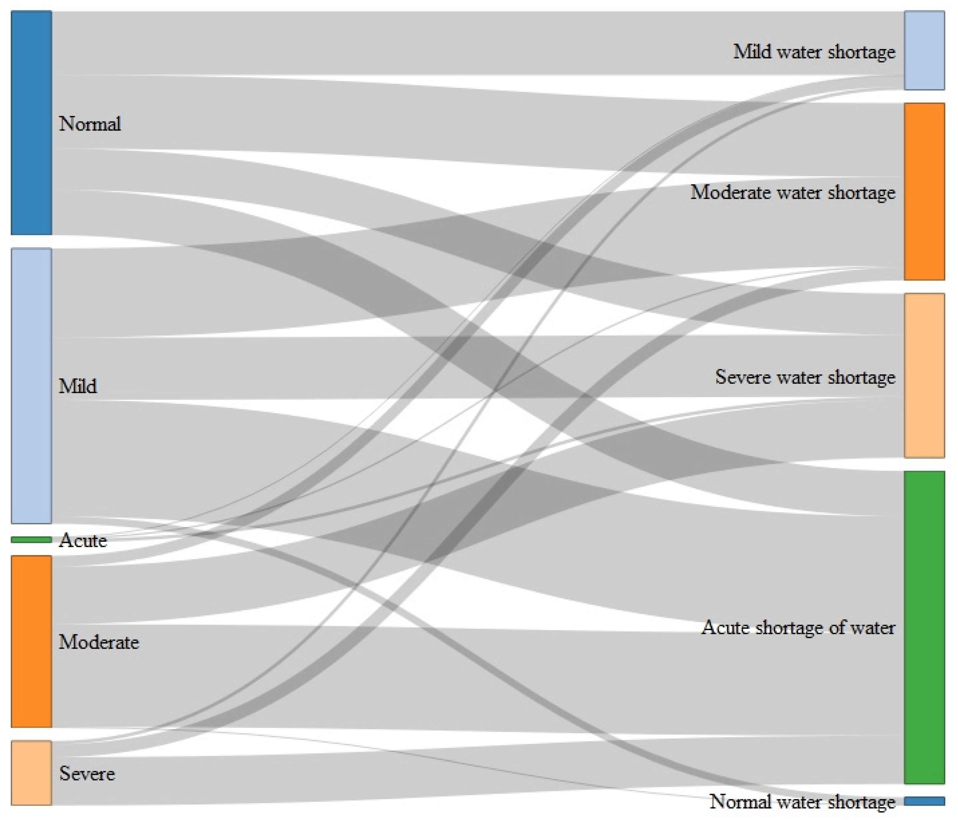
4.1.2. Characteristics of Moisture Profit and Loss Transition
During 2003–2015, there were relatively frequent mutual transitions of various types of water shortage in the Yanhe River Basin (Figure 2). Hereinto, the transition from normal water shortage to other water shortage types was greatest, and the normal water shortage mainly transferred into mild, moderate, and acute water shortages, of which the transition from normal to moderate water shortage had the largest area of 224 km2. The mild water shortage mainly transferred into moderate and acute water shortages, with areas of 271 and 355 km2, respectively; the moderate water shortage mainly transferred into severe and acute water shortages, with a transition area of 312 km2. The severe water shortage transferred into the acute water shortage with an area of 146 km2. The transition amplitudes of normal, mild, or acute water shortages to other water shortage types were large; the transfer-out area of normal and mild water shortage was larger than the transfer-in area, while the transfer-in area of acute water shortage was considerably larger than its transfer-out area.
4.1.3. Variation Trend of Moisture Profit and Loss Degree
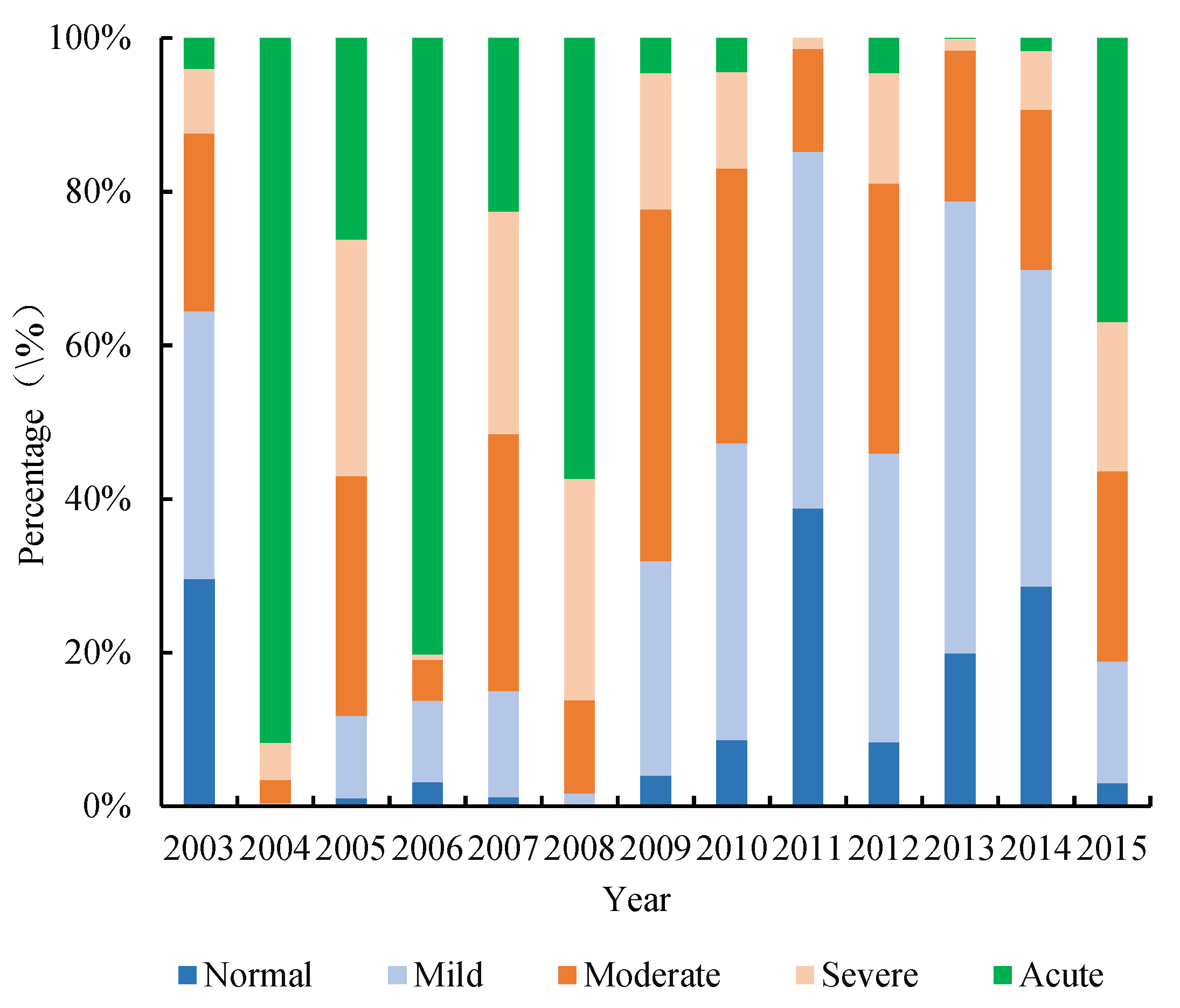
From 2003 to 2007, the water deficit situation in the Yanhe River Basin was significantly aggravated (Figure 3). In 2003, the water situation was mainly characterized by normal and mild water shortage, with no acute water shortage. The overall moisture profit and loss situation in the basin was good. In 2004, the area of the regions with acute water shortage increased sharply, and the proportion was as high as 91.75%. By 2007, the water situation was mainly characterized by moderate, severe, and acute water shortages, while there were no regions with normal water shortage. From 2007 to 2011, the farmland water deficit could be mitigated. The area of the regions with normal water shortage increased relatively slowly from 2007 to 2009, but increased sharply in 2010, and the water deficit situation exhibited an obvious ameliorating trend; the area of the regions with mild water shortage state decreased slightly in 2008, with a subsequent increase each year. The area of the regions with moderate water shortage state fluctuated, but its overall proportion decreased to some extent. The area of the regions with severe water shortage varied only slightly from 2007 to 2008 and significantly from 2009 to 2011, and its proportion decreased to 1.37% in 2011. The area of the regions with acute water shortage increased slightly in 2008 and then gradually decreased to zero in 2011, with an overall proportion increase by 32.97%. From 2011 to 2015, the farmland water deficit situation deteriorated again. The area of the regions under normal water shortage decreased drastically in 2012, with a subsequent slight increase in 2013 and an overall proportion decrease by up to 35.79%. The area of the regions with mild water shortage increased slightly in 2013 and then decreased gradually, with a percentage change of 30.52%, while the area under moderate water shortage changed only slightly. The area of the regions with severe water shortage decreased by 0.15% in 2013, with a subsequent gradual increase and an overall proportion increase by 18.05%, while the area of the regions under acute water shortage increased significantly in 2015, with a proportion increase by 35.27% compared to 2014.
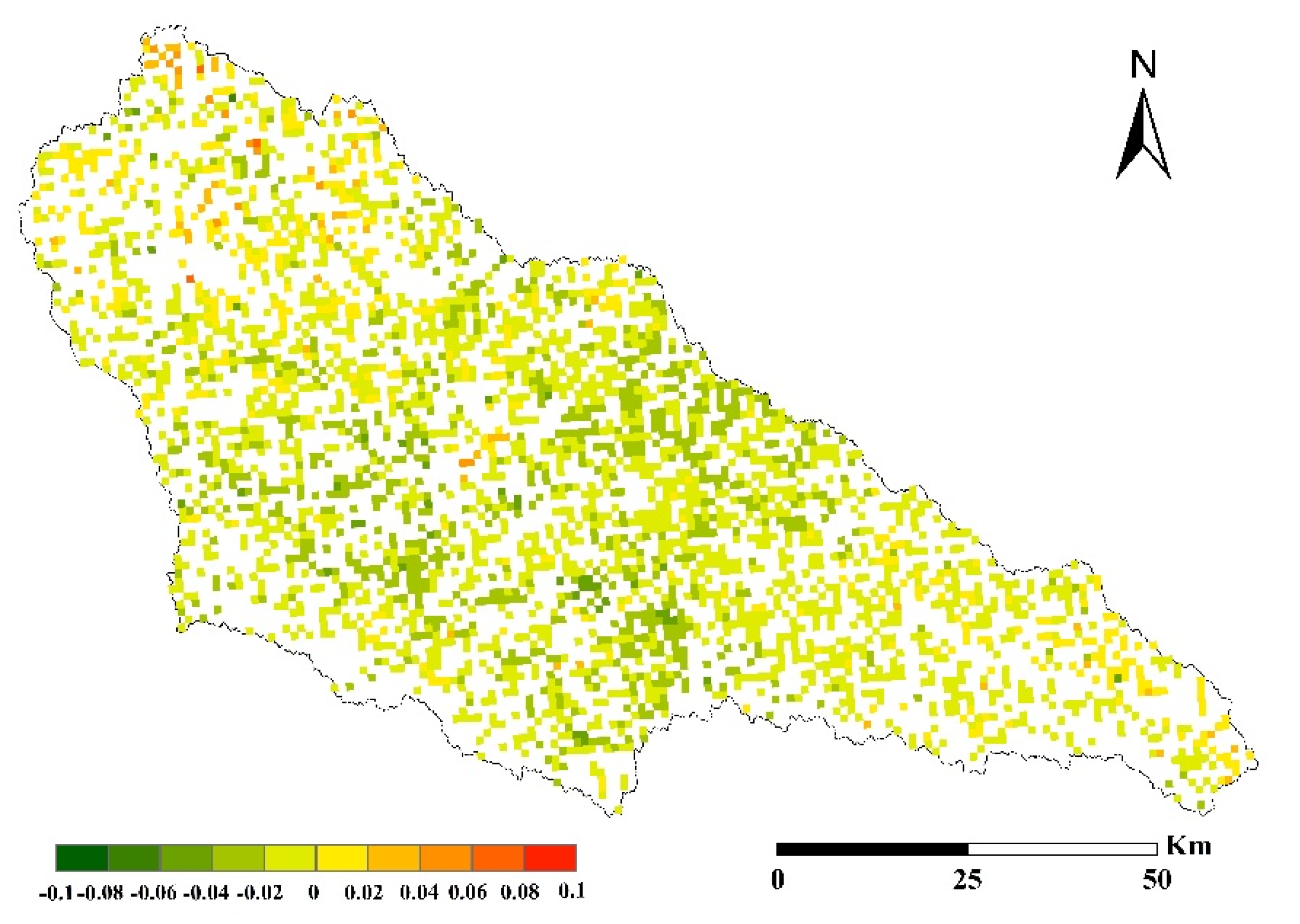
In order to more clearly show the trend of MPLD in 2003–2015, we calculated the trend of each grid unit (Figure 4). We can see that from 2003 to 2015, the water deficit in the upper and lower reaches of the Yanhe River Basin showed an intensifying trend, but a weakening trend in the middle reaches.
4.2. Spatial Distribution of Moisture Profit and Loss
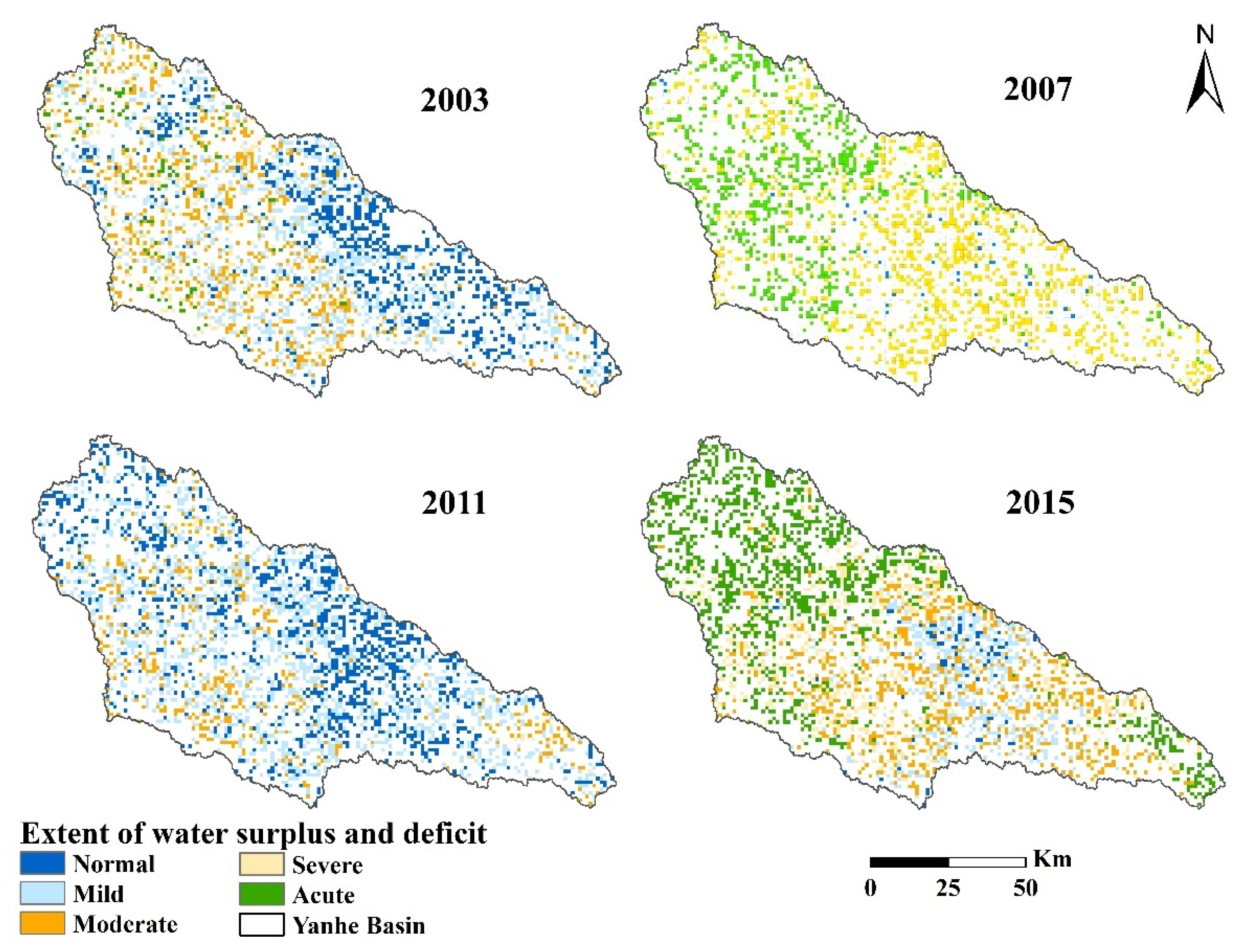
From 2003 to 2015, the Yanhe River Basin was characterized by water shortage, with negative moisture profit and loss values (Figure 5), suggesting that the natural precipitation in the basin was insufficient to meet water needs. In 2003, normal and mild water shortages dominated, while the area of the regions under moderate, severe, and acute water shortages was relatively small. Regions with acute water shortage were scattered throughout the Zhidan and Jingbian regions in the western part of the Yanhe River Basin, while the regions under normal water shortage were mainly distributed in the Yanan City and the north of Yanchang County. Based on the results of the statistical analysis, the average value of the MPLD index of the farmland in the basin was below 0.06, indicating normal water shortage (MPLD ≤ 0.15) and suggesting that the overall moisture profit and loss situation of the farmland was good in 2003. Up to 2007, the area of the regions under severe and acute water shortage increased sharply, which mainly manifested as the transformation of the spatial distribution of the regions with acute water shortage in the western part of the basin from a scattered distribution to a wider distribution, and the water shortage was acute in the regions Zhidan, Jingbian, and Ansai. In 2011, the water situation in these regions improved, and the Yanan City reached a normal water shortage situation. In 2015, the regions Zhidan and Ansai experienced moderate and acute water shortages, and the southeast of Yanchang County was characterized by acute water shortage.
5. Discussion
5.1. Factors Influencing MPLD Changes
5.1.1. Factors Influencing MPLD Changes
The changes in MPLD depend on precipitation and potential evapotranspiration, while the potential evapotranspiration is affected by meteorological factors such as air temperature, wind speed, humidity, and radiation quantity. In this study, we selected the six meteorological factors—precipitation, air pressure, radiation quantity, near-surface air specific humidity, air temperature, and wind speed to conduct regression analysis on the relationships between any of these six factors and the MPLD (Figure 6). The results show that precipitation and near-surface air specific humidity were significantly negatively correlated with the degree of moisture profit and loss (P < 0.05), and the increase in these factors could result in the decrease in MPLD, suggesting improved water conditions. Radiation quantity was significantly positively correlated with the degree of moisture profit and loss (P = 0.05), and an increase in radiation quantity could result in an increase in MPLD, indicating a deteriorating water condition. Other climatic factors showed no significant correlations with MPLD (P > 0.05). Thus, precipitation and near-surface air specific humidity are the dominant factors affecting moisture profit and loss in the Yanhe River Basin, while the relatively low amount of precipitation is the main reason for the water deficit situation in the Yanhe River Basin.
5.1.2. Changes in Impact Factors in Different Years
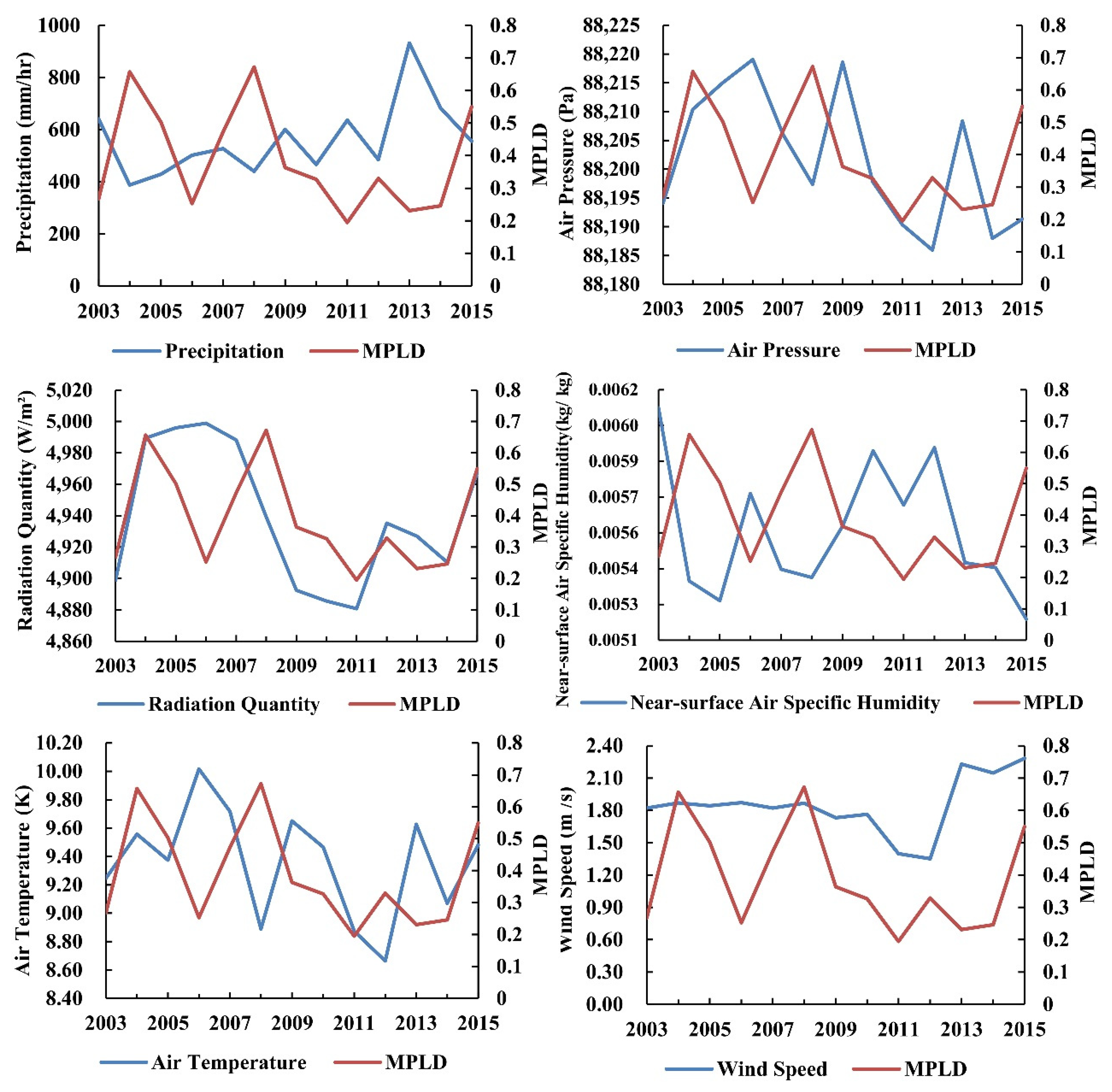
In order to clearly show which factors dominated the changes in MPLD, we plotted a line graph of six meteorological factors and MPLD changes (Figure 7). By comparing the trend of the line chart, we can clearly see that in 2007, precipitation, air pressure, near-surface air than humidity and air temperature are exactly opposite to the trend of MPLD, and the combination of the four causes MPLD to rise. In 2011, the content of combination changed, and the combination of precipitation, radiation, near-surface air specific humidity and wind speed led to a decline in MPLD. In 2015, precipitation, near-surface air combined with humidity and temperature led to an increase in MPLD.
5.1.3. Spatial Performance of Impact Factors on MPLD
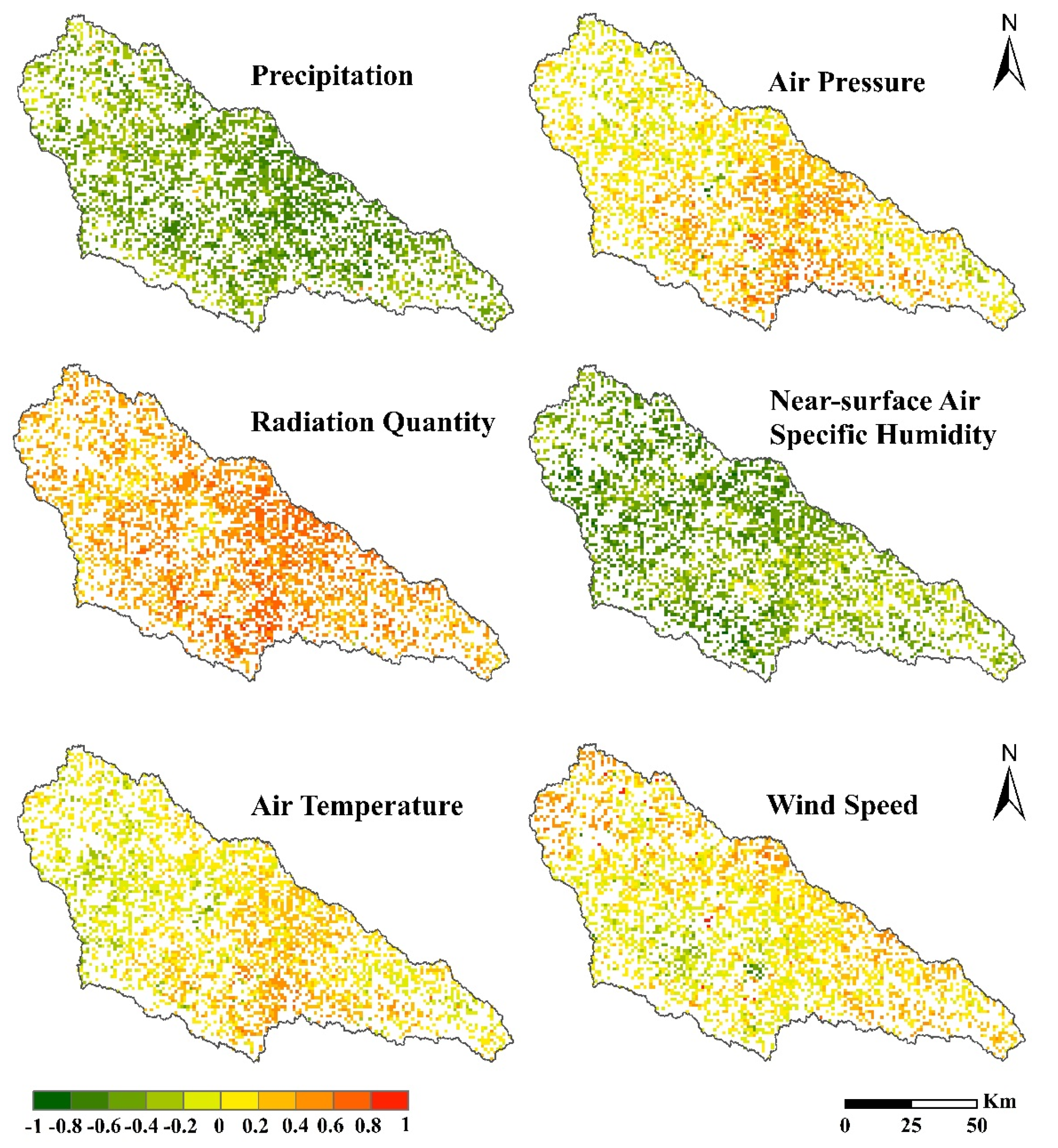
In order to clearly show the influence of meteorological factors on MPLD in the upstream, midstream and downstream of the basin, we also calculated the impact of meteorological factors on each grid unit on MPLD (Figure 8). We found that the impact of precipitation on the MPLD in the basin was large, while the impact of air pressure on the MPLD was small, and some high-value areas were only distributed in the middle and downstream. Radiation had a great influence on the downstream areas of the basin, but little on the upstream and downstream areas of the basin. The near-surface air had a greater impact than the upper and middle reaches of the wet-watershed, and had a small impact on the downstream of the basin. The midstream area in the river basin was greatly affected by the air temperature, while the upstream and downstream areas were less affected by this factor. The upper reaches of the basin were strongly affected by wind speed, while the middle and lower reaches only had some inhomogeneous scattered high-value areas.
5.2. Comparison with Previous Research
The previous studies on the changes in water surplus and loss in the Loess Plateau of China and the northwestern arid regions in China show that the water deficit situation in this region was grim, mainly as a result of climatic changes [43,44,45]. Meteorological factors such as precipitation, temperature and wind speed had a great influence on the change of water surplus and loss, especially precipitation which was the dominant factor influencing water evapotranspiration changes [46,47,48]. The study also indicated that some factors like temperature, solar radiation, and wind speed showed a positive correlation with changes in water profit and loss, while precipitation showed a negative correlation [49]. We compared our results on the water deficit situation in the Yanhe River Basin with previous research. These results were consistent with the results on the factors influencing moisture profit and loss in the Yanhe River Basin, precipitation was the meteorological factor with the most significant influence on the drought situation. The study area was located in the semi-arid region of northwestern China, with low annual precipitation. The seasonal distribution of precipitation was uneven, and rain mostly occurred from June to September. In recent years, the amount of precipitation decreased [50], especially in spring, summer, and autumn [2]. Hence, the water resources in the Yanhe River Basin were minimized. Under the influence of this factor, the water deficit situation in the Yanhe River Basin is becoming more and more severe.
5.3. Suggestions of Mitigating Water Shortages
To mitigate the water shortage in the Yanhe River Basin, one starting point might be the regulation of domestic water use, production water use, and ecological water use, combined with overall water resources protection. In the future, the Yanhe River Basin is predicted to be warmer and drier. On the other hand, with the acceleration of urbanization, the demand for agricultural and industrial water will continue to increase, making it necessary to focus on increasing the efficiency of water resources, and on optimizing water resources allocation to achieve maximum ecological and economic benefits [51]. We should, therefore, adjust the use pattern and use structure of water resources from the perspective of the benefit of the whole basin, reasonably exploit and use surface water and groundwater, improve the construction of supporting facilities of farmland water conservancy projects, and vigorously develop sustainable and water-saving agriculture. It is also important to intensify the protection of water resources and to prevent water pollution. A comprehensive improvement of industrial, agricultural, and domestic water use is important, along with adjusting the industrial structure and optimizing the industrial layout and scale in the basin. At present, the main vegetation types in the “Returning Farmland to Forest” project of the Yanhe River Basin are Pinus tabulaeformis and Robinia pseudoacacia plantations. However, because the water demands of these forest stands cannot be met, other tree species have appeared. This leads us to infer that the selection of adequate plant species is of significant importance, with the aim to minimize the water demand, thereby avoiding negative effects caused by the establishment of unsuitable species.
5.4. Uncertainty
The Uncertainty of this study mainly come from three aspects, one is the error comes from the calculation process of ET0, the other is the error of the ET data product used, and the third is the error caused by the interpolation of meteorological data. The ET0 calculation error is mainly due to the uncertainty of the model and the input parameters. The calculation process of ET0 is complicated and is greatly affected by meteorological data, land cover type and soil properties. Therefore, it must be simplified in the actual calculation process, which may lead to equation calculation errors. The second uncertainty of ET0 calculation is derived from the error of the input parameters. The data used for parameter estimation is mostly obtained by measurement. Instrument faults, different spatial and temporal resolutions, etc., during the measurement process may cause errors [52]. As the calculation of net radiation (Rn) parameter in the Penman–Monteith model. The net radiation (Rn) is the difference between the net solar radiation (Rns) and (Rnl). Since solar radiation is determined by factors such as solar constant, sun dip, geographical position and atmospheric transmittance, and ground height [42], some of the parameters used in the calculation of this parameter are applicable globally, and may bring some errors when applied to small areas. Studies have shown that the relative error of Rs calculated based on existing remote sensing or at flux tower sites data is about 10% [53,54]. The ET data used in this study was calculated by the Simplified Surface Energy Balance (SSEBop) model, which simplifies the surface energy balance equation and does not explicitly solve the sensible heat flux and geothermal flux. The simplification of the SSEBop model leads to uncertainties in the model output process [55]. Second is the model output error due to the uncertainty of the input variable error. For example, the studies show that under stable atmospheric conditions, the Ts error of all stations is generally within 1k [56]. However, in semi-arid and arid regions, the error may be as high as 5k due to emissivity and albedo [38]. The error about meteorological data mainly comes from interpolation, and the application of interpolation will inevitably bring some errors by any means. In this study, we used AUSPLIN (an interpolation program) to interpolate meteorological data. In the interpolation process, we added the consideration of topographical factors, which minimized the occurrence of errors.
6. Conclusions
Using the moisture profit and loss degree index model, we analyzed the spatio-temporal distribution characteristics and the corresponding factors influencing moisture profits and losses in the Yanhe River Basin from 2003 to 2015. Overall, the moisture profit and loss degree of farmland varied dramatically, and the water deficit situation presented a deteriorating trend from 2013 to 2015 except for 2011 and 2013. The area of the regions with normal and acute water shortage changed most significantly, while the change rates of the areas with severe and acute water shortage were highest. The main factor influencing the water condition was precipitation, followed by radiation and near-surface air specific humidity. How to reasonably allocate and use the limited water resources [57], how to relieve the tense situation of water resources, and how to improve the sustainability of agricultural development are the key points when dealing with the perennial water deficit situation in the Yanhe River Basin.
The water situation in the basin was characterized by water shortage, with a non-uniform spatial distribution. In the recent 13 years, the spatial distribution of the moisture profit and loss in the river basin generally presented a progressively decreasing trend from northwest to southeast. The water deficit was most severe in the northwestern region of the basin, mainly in the areas around Zhidan and Ansai. In the central region of the basin, water profits and losses changed slowly. In 2015, the overall water situation in the basin was grim, and the regions with high MPLD index values were concentrated in some areas. In this context, the government should strengthen the management of water resources in the river basin, intensify the protection of water resources, promote the construction of agricultural water conservation facilities, and continue to implement ecological construction projects [58], with the overall aim to achieve higher economic, social, and ecological benefits.
Author Contributions
W.S. designed the research, while Z.W. processed the data, developed the methodology, performed the research and wrote the manuscript. W.S. reviewed the paper and supported the analyses, while W.S., X.Y. and L.Y. supervised the research and contributed with discussions and scientific advice.
Funding
The research was supported by the Second Tibetan Plateau Scientific Expedition and Research Program (STEP) (Grant No. 2019QZKK060300), the Strategic Priority Research Program of Chinese Academy of Sciences (Grant No. XDA20040201), the National Key Research and Development Plan of China (Grant No. 2016YFA0602402), the Projects of National Natural Science Foundation of China (Grant No. 41671177) and the Project of Research of Standards Drafting Expert Database from China National Institute of Standardization.
Conflicts of Interest
The authors declare no conflicts of interest.
Appendix A. Meteorological Parameters of the Penman–Monteith Formula
This appendix discusses the source, measurement and computation of all data required for the calculation of the reference evapotranspiration by means of the FAO Penman–Monteith method [9].
- Mean saturation vapor pressure (es)
As saturation vapor pressure is related to air temperature, it can be calculated from the air temperature. The relationship is expressed by:
where e°(T) is the saturation vapor pressure at the air temperature T [kPa], T is the air temperature [°C], exp[..] is the 2.7183 (base of natural logarithm) raised to the power [..].
Due to the non-linearity of the above equation, the mean saturation vapor pressure should be computed as the mean between the saturation vapor pressure at the mean daily maximum and minimum air temperatures for that period:
- 2.
- Slope of saturation vapor pressure curve (Δ)
For the calculation of evapotranspiration, the slope of the relationship between saturation vapor pressure and temperature, Δ, is required. The slope of the curve at a given temperature is given by:
where Δ is the slope of saturation vapor pressure curve at air temperature T [kPa °C–1], T is the air temperature [°C], exp[..] is the 2.7183 (base of natural logarithm) raised to the power [..].
- 3.
- Actual vapor pressure (ea) derived from relative humidity data
The actual vapor pressure can also be calculated from the relative humidity. Depending on the availability of the humidity data, different equations should be used.
where ea is the actual vapor pressure [kPa], e°(Tmin) is the saturation vapor pressure at daily minimum temperature [kPa], e°(Tmax) is the saturation vapor pressure at daily maximum temperature [kPa], RHmax is the maximum relative humidity [%], RHmin is the minimum relative humidity [%].
The relative humidity (RH) expresses the degree of saturation of the air as a ratio of the actual (ea) to the saturation (eo(T)) vapor pressure at the same temperature (T):
- 4.
- Net radiation (Rn)
The net radiation (Rn) is the difference between the incoming net shortwave radiation (Rns) and the outgoing net longwave radiation (Rnl):
The net shortwave radiation resulting from the balance between incoming and reflected solar radiation is given by:
where Rns is the net solar or shortwave radiation [MJ m–2 day–1], is the albedo or canopy reflection coefficient, which is 0.23 for the hypothetical grass reference crop [dimensionless], Rs is the the incoming solar radiation [MJ m−2 day−1]. Rns is expressed in the above equation in MJ m−2 day−1.
The rate of longwave energy emission is proportional to the absolute temperature of the surface raised to the fourth power. This relation is expressed quantitatively by the Stefan–Boltzmann law. The net energy flux leaving the earth’s surface is, however, less than that emitted and given by the Stefan–Boltzmann law due to the absorption and downward radiation from the sky. As humidity and cloudiness play an important role, the Stefan–Boltzmann law is corrected by these two factors when estimating the net outgoing flux of longwave radiation. It is thereby assumed that the concentrations of the other absorbers are constant:
where Rnl is the net outgoing longwave radiation [MJ m–2 day–1], σ is the Stefan–Boltzmann constant [4.903 10–9 MJ K–4 m-2 day–1], Tmax,K is the maximum absolute temperature during the 24-h period [K = °C + 273.16], Tmin,K is the minimum absolute temperature during the 24-h period [K = °C + 273.16], ea is the actual vapor pressure [kPa], Rs/Rso is the relative shortwave radiation (limited to ≤1.0).
If the solar radiation, , is not measured, it can be calculated with the Angstrom formula, which relates solar radiation to extraterrestrial radiation and relative sunshine duration:
where is the solar or shortwave radiation [MJ m–2 day–1], n is the actual duration of sunshine [hour], N is the maximum possible duration of sunshine or daylight hours [hour], n/N is the relative sunshine duration [-], is the extraterrestrial radiation [MJ m–2 day–1], is the regression constant, expressing the fraction of extraterrestrial radiation reaching the earth on overcast days (n = 0), + is the fraction of extraterrestrial radiation reaching the earth on clear days (n = N).
The calculation of the clear-sky radiation, , when n = N, is required for computing net longwave radiation.
For near sea level or when calibrated values for and are available:
where is the clear-sky solar radiation [MJ m–2 day–1], + is the fraction of extraterrestrial radiation reaching the earth on clear-sky days (n = N).
When calibrated values for and are not available:
where z is the station elevation above sea level [m].
- 5.
- Soil heat flux (G)
Complex models are available to describe soil heat flux. Because soil heat flux is small compared to Rn, particularly when the surface is covered by vegetation and calculation time steps are 24 h or longer, a simple calculation procedure is presented here for long time steps, based on the idea that the soil temperature follows air temperature:
where G is the soil heat flux [MJ m–2 day–1], Cs is the soil heat capacity [MJ m–3 °C–1], Ti is the air temperature at time i [°C], Ti-1 is the air temperature at time i-1 [°C], Δt is the length of time interval [day], Δz is the effective soil depth [m].
- 6.
- Psychrometric constant (γ)
The psychrometric constant, γ, is given by:
where γ is the psychrometric constant [kPa °C–1], is the atmospheric pressure [kPa], is the latent heat of vaporization, 2.45 [MJ kg-1], is the specific heat at constant pressure, 1.013 10–3 [MJ kg-1 °C-1], is the ratio molecular weight of water vapor/dry air = 0.622.
- 7.
- Air Temperature
Due to the non-linearity of humidity data required in the FAO Penman–Monteith equation, the vapor pressure for a certain period should be computed as the mean between the vapor pressure at the daily maximum and minimum air temperatures of that period. For standardization, Tmean for 24-h periods is defined as the mean of the daily maximum (Tmax) and minimum temperatures (Tmin) rather than as the average of hourly temperature measurements.
- 8.
- Wind profile relationship
Wind speeds measured at different heights above the soil surface are different. Surface friction tends to slow down wind passing over it. Wind speed is slowest at the surface and increases with height. For this reason, anemometers are placed at a chosen standard height, i.e., 10m in meteorology and 2 or 3m in agrometeorology. For the calculation of evapotranspiration, wind speed measured at 2m above the surface is required. To adjust wind speed data obtained from instruments placed at elevations other than the standard height of 2 m, a logarithmic wind speed profile may be used for measurements above a short grassed surface:
where u2 is the wind speed at 2 m above ground surface [m s–1], uz is the measured wind speed at z m above ground surface [m s−1], z is the height of measurement above ground surface [m].
Appendix B. Actual Evapotranspiration (ETa)
The SSEBop model was developed to estimate actual evapotranspiration (ETa) in space from pixel to regional scales and in time from daily to annual scales using remotely sensed observations and climatological data. The SSEBop model can be mathematically expressed as follows [55]:
where Rns is clear-sky net shortwave radiation (MJ/m2/d) depending upon albedo (α) (unitless), incoming solar radiation Rs (MJ/m2/d), extraterrestrial radiation Ra, and elevation z (m), Rnl is clear-sky net longwave radiation (MJ/m2/d) based on minimum temperature (Tmin) (K) and maximum temperature (Tmax) (K), rah is aerodynamic resistance for heat (s/m), is air density (kg/m3) depending on daily average temperature Ta (K) and elevation z (m), and Cp is specific heat of air at constant pressure (~1003 J/kg/K).
References
- Intergovernmental Panel on Climate Change (IPCC). Climate Change 2013: The Physical Science Basis. Contribution of Working Group I to the Fifth Assessment Report of the Intergovernmental Panel on Climate Change; Stocker, T.F., Qin, D., Plattner, G.-K., Tignor, M., Allen, S.K., Boschung, J., Nauels, A., Xia, Y., Bex, V., Midgley, P.M., Eds.; Cambridge University Press: Cambridge, UK; New York, NY, USA, 2013; p. 1535. [Google Scholar] [CrossRef]
- Labat, D.; Goddéris, Y.; Probst, J.L.; Guyot, J.L. Evidence for global runoff increase related to climate warming. Adv. Water Resour. 2004, 27, 631–642. [Google Scholar] [CrossRef]
- Zhu, Q.; Luo, Y.; Xu, Y.-P.; Tian, Y.; Yang, T. Satellite soil moisture for agricultural drought monitoring: Assessment of SMAP-derived soil water deficit index in Xiang River Basin, China. Remote Sens. 2019, 11, 362. [Google Scholar] [CrossRef]
- Wu, L.; Liu, X.; Ma, X.-Y. Spatiotemporal distribution of rainfall erosivity in the Yanhe River watershed of hilly and gully region, Chinese Loess Plateau. Environ. Earth Sci. 2016, 75, 315. [Google Scholar] [CrossRef]
- Yang, R.-J.; Fu, B.-J.; Liu, G.-H.; Ma, K.-M. Research on the relationship between water and eco-environment construction in Loess Hilly and Gully regions. Huanjing Kexue 2004, 25, 37–42. [Google Scholar] [PubMed]
- Zhen, L. The national census for soil erosion and dynamic analysis in China. Int. Soil Water Conserv. Res. 2013, 1, 12–18. [Google Scholar] [CrossRef] [Green Version]
- Zhang, L.; Potter, N.; Hickel, K.; Zhang, Y.; Shao, Q. Water balance modeling over variable time scales based on the Budyko framework—Model development and testing. J. Hydrol. 2008, 360, 117–131. [Google Scholar] [CrossRef]
- Piao, S.; Ciais, P.; Huang, Y.; Shen, Z.; Peng, S.; Li, J.; Zhou, L.; Liu, H.; Ma, Y.; Ding, Y.; et al. The impacts of climate change on water resources and agriculture in China. Nature 2010, 467, 43–51. [Google Scholar] [CrossRef] [PubMed]
- Allen, R.G.; Pereira, L.S.; Raes, D.; Smith, M. Crop Evapotranspiration-Guidelines for Computing Crop Water Requirements; FAO Irrigation and Drainage Paper 56; Food and Agriculture Organization of the United Nations (FAO): Rome, Italy, 1998. [Google Scholar]
- Trajkovic, S. Hargreaves versus Penman-Monteith under humid conditions. J. Irrig. Drain. Eng. 2007, 133, 38–42. [Google Scholar] [CrossRef]
- Yin, Y.; Wu, S.; Zheng, D.; Yang, Q. Radiation calibration of FAO56 Penman–Monteith model to estimate reference crop evapotranspiration in China. Agric. Water Manag. 2008, 95, 77–84. [Google Scholar] [CrossRef]
- Deliang, C.; Ge, G.; Chong-Yu, X.; Jun, G.; Guoyu, R. Comparison of the Thornthwaite method and pan data with the standard Penman-Monteith estimates of reference evapotranspiration in China. Clim. Res. 2005, 28, 123–132. [Google Scholar]
- Sumner, D.M.; Jacobs, J.M. Utility of Penman–Monteith, Priestley–Taylor, reference evapotranspiration, and pan evaporation methods to estimate pasture evapotranspiration. J. Hydrol. 2005, 308, 81–104. [Google Scholar] [CrossRef]
- Ai, Z.; Yang, Y. Modification and validation of Priestley–Taylor model for estimating cotton evapotranspiration under plastic mulch condition. J. Hydrometeorol. 2016, 17, 1281–1293. [Google Scholar] [CrossRef]
- Kashyap, P.S.; Panda, R.K. Evaluation of evapotranspiration estimation methods and development of crop-coefficients for potato crop in a sub-humid region. Agric. Water Manag. 2001, 50, 9–25. [Google Scholar] [CrossRef]
- Shaozhong, K.; Huanjie, C.; Jianhua, Z. Estimation of maize evapotranspiration under water deficits in a semiarid region. Agric. Water Manag. 2000, 43, 1–14. [Google Scholar] [CrossRef]
- Croitoru, A.-E.; Piticar, A.; Dragotă, C.S.; Burada, D.C. Recent changes in reference evapotranspiration in Romania. Glob. Planet. Chang. 2013, 111, 127–136. [Google Scholar] [CrossRef]
- Abdelhadi, A.W.; Hata, T.; Tanakamaru, H.; Tada, A.; Tariq, M.A. Estimation of crop water requirements in arid region using Penman–Monteith equation with derived crop coefficients: A case study on Acala cotton in Sudan Gezira irrigated scheme. Agric. Water Manag. 2000, 45, 203–214. [Google Scholar] [CrossRef]
- Ai, Z.; Yang, Y.; Wang, Q.X.; Manevski, K.; Wang, Q.; Hu, Q.; Eer, D.; Wang, J. Characteristics and influencing factors of crop coefficient for drip-irrigated cotton under plastic mulch conditions in arid environment. J. Agric. Meteorol. 2017, 74, 1–8. [Google Scholar] [CrossRef]
- Allen, R.G. Using the FAO-56 dual crop coefficient method over an irrigated region as part of an evapotranspiration intercomparison study. J. Hydrol. 2000, 229, 27–41. [Google Scholar] [CrossRef]
- Tong, L.; Kang, S.; Zhang, L. Temporal and spatial variations of evapotranspiration for spring wheat in the Shiyang river basin in northwest China. Agric. Water Manag. 2007, 87, 241–250. [Google Scholar] [CrossRef]
- Howell, T.A.; Evett, S.R. The Penman-Monteith method. In Evapotranspiration: Determination of Consumptive Use in Water Rights Proceedings; Continuing Legal Education in Colorado, Inc.: Denver, CO, USA, 2004. [Google Scholar]
- Mahmood, R.; Hubbard, K.G. Simulating sensitivity of soil moisture and evapotranspiration under heterogeneous soils and land uses. J. Hydrol. 2003, 280, 72–90. [Google Scholar] [CrossRef]
- Rubio, J.G.; Belmonte, A.C.; Enguita, L.F.; Alcázar, I.A.; Mancebo, M.B.; Campos, I.; Rubio, R.B. Remote sensing-based soil water balance for irrigation water accounting at the Spanish Iberian Peninsula. Proc. Int. Assoc. Hydrol. Sci. 2018, 380, 29–35. [Google Scholar] [Green Version]
- Bandyopadhyay, P.K.; Mallick, S. Actual evapotranspiration and crop coefficients of wheat (Triticum aestivum) under varying moisture levels of humid tropical canal command area. Agric. Water Manag. 2003, 59, 33–47. [Google Scholar] [CrossRef]
- Teixeira, A.H.D.C. Determining regional actual evapotranspiration of irrigated crops and natural vegetation in the São Francisco River Basin (Brazil) using remote sensing and Penman-Monteith equation. Remote Sens. 2010, 2, 1287–1319. [Google Scholar] [CrossRef]
- Narasimhan, B.; Srinivasan, R. Development and evaluation of Soil Moisture Deficit Index (SMDI) and Evapotranspiration Deficit Index (ETDI) for agricultural drought monitoring. Agric. For. Meteorol. 2005, 133, 69–88. [Google Scholar] [CrossRef]
- Dai, A.; Trenberth, K.E.; Qian, T. A global dataset of palmer drought severity index for 1870–2002: Relationship with soil moisture and effects of surface warming. J. Hydrometeorol. 2004, 5, 1117–1130. [Google Scholar] [CrossRef]
- Gong, L.; Xu, C.-Y.; Chen, D.; Halldin, S.; Chen, Y.D. Sensitivity of the Penman–Monteith reference evapotranspiration to key climatic variables in the Changjiang (Yangtze River) basin. J. Hydrol. 2006, 329, 620–629. [Google Scholar] [CrossRef]
- Kruijt, B.; Witte, J.-P.M.; Jacobs, C.M.J.; Kroon, T. Effects of rising atmospheric CO2 on evapotranspiration and soil moisture: A practical approach for the Netherlands. J. Hydrol. 2008, 349, 257–267. [Google Scholar] [CrossRef]
- Li, J.; Zhou, Z. Landscape pattern and hydrological processes in Yanhe River basin of China. Acta Geogr. Sin. 2014, 69, 933–944. [Google Scholar] [CrossRef]
- Zheng, Z.; Fu, B.; Feng, X. GIS-based analysis for hotspot identification of tradeoff between ecosystem services: A case study in Yanhe Basin, China. Chin. Geogr. Sci. 2016, 26, 466–477. [Google Scholar] [CrossRef] [Green Version]
- Zheng, Z.; Fu, B.; Hu, H.; Sun, G. A method to identify the variable ecosystem services relationship across time: A case study on Yanhe Basin, China. Landsc. Ecol. 2014, 29, 1689–1696. [Google Scholar] [CrossRef]
- EARTHDATA. Available online: https://earthdata.nasa.gov/ (accessed on 10 June 2018).
- China Meteorological Data(CMD). Available online: http://data.cma.cn/ (accessed on 23 June 2018).
- He, J.; Yang, K. China Meteorological Forcing Dataset; Cold and Arid Regions Science Data Center at Lanzhou: Lanzhou, China, 2011. [Google Scholar]
- U.S. Geological Survey (USGS). Available online: https://earlywarning.usgs.gov/ (accessed on 8 July 2018).
- Senay, G.B.; Bohms, S.; Singh, R.K.; Gowda, P.H.; Velpuri, N.M.; Alemu, H.; Verdin, J.P. Operational evapotranspiration mapping using remote sensing and weather datasets: A new parameterization for the SSEB approach. JAWRA 2013, 49, 577–591. [Google Scholar] [CrossRef]
- Chinese Academy of Sciences. The Data Center for Resources and Environmental Sciences (DCRES). Available online: http://www.resdc.cn/ (accessed on 1 June 2018).
- Torres, A.F.; Walker, W.R.; McKee, M. Forecasting daily potential evapotranspiration using machine learning and limited climatic data. Agric. Water Manag. 2011, 98, 553–562. [Google Scholar] [CrossRef]
- Allen, R.; Smith, M.; Pereira, L.; Pruitt, W.O. Proposed revision to the FAO procedure for estimating crop water requirements. Acta Hortic. 1997, 449, 17–33. [Google Scholar] [CrossRef]
- Senay, G.B. Modeling landscape evapotranspiration by integrating land surface phenology and a water balance algorithm. Algorithms 2008, 1, 52–68. [Google Scholar] [CrossRef]
- Wang, W.; Shao, Q.; Peng, S.; Xing, W.; Yang, T.; Luo, Y.; Yong, B.; Xu, J. Reference evapotranspiration change and the causes across the Yellow River Basin during 1957–2008 and their spatial and seasonal differences. Water Resour. Res. 2012, 48. [Google Scholar] [CrossRef]
- Gao, G.; Chen, D.; Ren, G.; Chen, Y.; Liao, Y. Spatial and temporal variations and controlling factors of potential evapotranspiration in China: 1956–2000. J. Geogr. Sci. 2006, 16, 3–12. [Google Scholar] [CrossRef]
- Huo, Z.; Dai, X.; Feng, S.; Kang, S.; Huang, G. Effect of climate change on reference evapotranspiration and aridity index in arid region of China. J. Hydrol. 2013, 492, 24–34. [Google Scholar] [CrossRef]
- Liu, X.; Zhang, D. Trend analysis of reference evapotranspiration in Northwest China: The roles of changing wind speed and surface air temperature. Hydrol. Process. 2013, 27, 3941–3948. [Google Scholar] [CrossRef]
- Li, C.; Wu, P.T.; Li, X.L.; Zhou, T.W.; Sun, S.K.; Wang, Y.B.; Luan, X.B.; Yu, X. Spatial and temporal evolution of climatic factors and its impacts on potential evapotranspiration in Loess Plateau of Northern Shaanxi, China. Sci. Total Environ. 2017, 589, 165–172. [Google Scholar] [CrossRef]
- Ning, T.; Li, Z.; Liu, W.; Han, X. Evolution of potential evapotranspiration in the northern Loess Plateau of China: Recent trends and climatic drivers. Int. J. Climatol. 2016, 36, 4019–4028. [Google Scholar] [CrossRef]
- Zhang, D.; Liu, X.; Hong, H. Assessing the effect of climate change on reference evapotranspiration in China. Stoch. Environ. Res. Risk Assess. 2013, 27, 1871–1881. [Google Scholar] [CrossRef]
- Liu, Q.; Yang, Z.; Cui, B. Spatial and temporal variability of annual precipitation during 1961–2006 in Yellow River Basin, China. J. Hydrol. 2008, 361, 330–338. [Google Scholar] [CrossRef]
- Zhou, Q.; Deng, X.; Wu, F.; Li, Z.; Song, W. Participatory irrigation management and irrigation water use efficiency in maize production: Evidence from Zhangye City, Northwestern China. Water 2017, 9, 822. [Google Scholar] [CrossRef]
- Ferguson, C.R.; Sheffield, J.; Wood, E.F.; Gao, H. Quantifying uncertainty in a remote sensing-based estimate of evapotranspiration over continental USA. Int. J. Remote Sens. 2010, 31, 3821–3865. [Google Scholar] [CrossRef]
- Glenn, E.P.; Huete, A.R.; Nagler, P.L.; Hirschboeck, K.K.; Brown, P. integrating remote sensing and ground methods to estimate evapotranspiration. Crit. Rev. Plant Sci. 2007, 26, 139–168. [Google Scholar] [CrossRef]
- Kalma, J.D.; McVicar, T.R.; McCabe, M.F. Estimating land surface evaporation: A review of methods using remotely sensed surface temperature data. Surv. Geophys. 2008, 29, 421–469. [Google Scholar] [CrossRef]
- Chen, M.; Senay, G.B.; Singh, R.K.; Verdin, J.P. Uncertainty analysis of the Operational Simplified Surface Energy Balance (SSEBop) model at multiple flux tower sites. J. Hydrol. 2016, 536, 384–399. [Google Scholar] [CrossRef] [Green Version]
- Hulley, G.C.; Hughes, C.G.; Hook, S.J. Quantifying uncertainties in land surface temperature and emissivity retrievals from ASTER and MODIS thermal infrared data. J. Geophys. Res. Atmos. 2012, 117. [Google Scholar] [CrossRef] [Green Version]
- Wang, X.; Xie, H. A review on applications of remote sensing and geographic information systems (GIS) in water resources and flood risk management. Water 2018, 10, 608. [Google Scholar] [CrossRef]
- Liu, Y.; Song, W.; Deng, X. Spatiotemporal patterns of crop irrigation water requirements in the Heihe River Basin, China. Water 2017, 9, 616. [Google Scholar] [CrossRef]
Figure 1.
Location of the Yanhe River Basin, Loess Plateau, China.

Figure 2.
Moisture profit and loss transitions in the Yanhe River Basin from 2007–2011.

Figure 3.
Proportions of different moisture profit and loss levels in the Yanhe River Basin from 2003 to 2015.
Figure 3.
Proportions of different moisture profit and loss levels in the Yanhe River Basin from 2003 to 2015.

Figure 4.
Spatial distribution map of moisture profit and loss degree (MPLD) change trend in the Yanhe River Basin from 2003 to 2015.
Figure 4.
Spatial distribution map of moisture profit and loss degree (MPLD) change trend in the Yanhe River Basin from 2003 to 2015.

Figure 5.
Spatial distribution of area changes at different levels of moisture profit and loss in the Yanhe River Basin in 2003, 2007, 2011, and 2015.
Figure 5.
Spatial distribution of area changes at different levels of moisture profit and loss in the Yanhe River Basin in 2003, 2007, 2011, and 2015.

Figure 6.
Spatial correlation coefficients of the water budget for different meteorological factors in the Yanhe River Basin (the grey zone represents the 95% confidence interval of the fitted line.).
Figure 6.
Spatial correlation coefficients of the water budget for different meteorological factors in the Yanhe River Basin (the grey zone represents the 95% confidence interval of the fitted line.).

Figure 7.
Changes of various influencing factors and MPLD in different years.

Figure 8.
Spatial distribution of correlation coefficients between MPLD and meteorological factors.


Table 1.
Moisture changes in the Yanhe River Basin from 2003–2015 (km2, %).
| 2003 | 2015 | 2003–2015 | ||||
|---|---|---|---|---|---|---|
| Area | Proportion | Area | Proportion | Variation Quantity | Variation Rate | |
| Normal water shortage | 879 | 29.61 | 93 | 3.04 | –786 | –89.42 |
| Mild water shortage | 1034 | 34.83 | 485 | 15.85 | –549 | –53.09 |
| Moderate water shortage | 687 | 23.14 | 757 | 24.75 | 70 | 10.19 |
| Severe water shortage | 251 | 8.45 | 594 | 19.42 | 343 | 136.65 |
| Acute water shortage | 118 | 3.97 | 1130 | 36.94 | 1,012 | 857.63 |
© 2019 by the authors. Licensee MDPI, Basel, Switzerland. This article is an open access article distributed under the terms and conditions of the Creative Commons Attribution (CC BY) license (http://creativecommons.org/licenses/by/4.0/).
Share and Cite
MDPI and ACS Style
Wang, Z.; Song, W.; Yuan, X.; Yin, L. Spatio-Temporal Variations in Farmland Water Conditions in the Yanhe River Basin. Water 2019, 11, 2234. https://doi.org/10.3390/w11112234
AMA Style
Wang Z, Song W, Yuan X, Yin L. Spatio-Temporal Variations in Farmland Water Conditions in the Yanhe River Basin. Water. 2019; 11(11):2234. https://doi.org/10.3390/w11112234
Chicago/Turabian StyleWang, Zhanyun, Wei Song, Xuefeng Yuan, and Lichang Yin. 2019. "Spatio-Temporal Variations in Farmland Water Conditions in the Yanhe River Basin" Water 11, no. 11: 2234. https://doi.org/10.3390/w11112234
Note that from the first issue of 2016, this journal uses article numbers instead of page numbers. See further details here.