Estimating Environmental Preferences of Freshwater Pelagic Fish Using Hydroacoustics and Satellite Remote Sensing

Abstract

In this study, a remote sensing-based method of mapping and predicting fish spatial distribution in inland waters is developed. A combination of Earth Observation data, in-situ measurements, and hydroacoustics is used to relate fish biomass distribution and water-quality parameters along the longitudinal transect of the Římov Reservoir (Czech Republic) using statistical and machine learning techniques. Parameter variations and biomass distribution are estimated and validated, and apparent trends are explored and discussed, together with potential limitations and weaknesses. Water-quality parameters exhibit longitudinal gradients along the reservoir, while calculations reveal a distinct fish assemblage pattern observed as a patchy overall biomass distribution. Although the proposed methodology has a great potential for sustainable water management, careful planning is needed to ensure the simultaneous acquisition of remote sensing and in-situ data to maximize calibration accuracy.

1. Introduction

Aimed at the sustainable management of freshwater ecosystems, several directives and management plans have been developed and implemented at the international, national, and regional level [1,2]. In Europe, the Water Framework Directive 2000/60/EC [3] calls for all natural aquatic ecosystems to achieve a “good” ecological status. However, methodologies adopted by researchers for the monitoring of freshwater fish stocks, such as gillnetting, require high effort, result in a reduction of fish biomass, and potentially fail to reflect the variability of fish density among lakes.

Taking into account that fish fauna is considered an ecological quality element in the aforementioned Directive, insofar as regards the assessment of the ecological status of water bodies, it has been supported that satellite imagery combined with fish monitoring techniques expand our understanding and lead to improved inferences with respect to water quality assessment [4]. With the synergy of geographical information systems (GIS) technologies, the combined application of satellite imagery and hydroacoustic data can yield a versatile methodology to study and model complex interactions between fish and their natural habitats.

At the same time, Earth Observation (EO) from space has become an increasingly important tool for freshwater resource managers and researchers in government agencies, conservation organizations, and industry [5]. Remote sensors on board satellites provide a systematic, synoptic view of earth cover at regular time intervals and are useful for biological monitoring of freshwater ecosystems. Satellite data are a powerful tool to predict many physico-chemical and biological water parameters such as water temperature, number of suspended solids, or primary productivity [6]. However, fish, like some other aquatic organisms, are not directly detectable from satellite data. To use satellite data for the assessment of fish biomass, relationships between water parameters that can be detected from satellite and fish distribution must be found. To calibrate a model, fish data obtained by other methods are also necessary.

Together, satellite-based EO and hydroacoustics are non-invasive techniques that can be utilized for fast, spatially precise mapping of land/water surface properties. Coupled with GIS, both techniques can provide comparable visualizations of patterns of these observed properties and their changes in space and time [7,8], thereby creating an ideal opportunity for analysis, evaluation, and decision-making processes. That is why the significance of these tools further increases in the face of scientific, societal, and political demands to understand processes and interactions within our environment.

The availability of the long-term data makes the Římov Reservoir a suitable model for the investigation of spatial patterns in water quality parameters and fish distribution. The reservoir is a highly heterogeneous environment with pronounced longitudinal gradients in various physical, chemical, and biological parameters. Typically, three zones can be recognized along the longitudinal axis of a reservoir [9]. The shallow riverine zone close to the river inflow is characterized by high flow, turbidity, and nutrient concentration. Thermal stratification is usually weak and often disrupted by high inflow episodes. In the transition part of the reservoir, phytoplankton biomass increases due to decreasing flow velocity, increased water residence time, high nutrients concentrations, and sufficient light availability. As a result, the transition zone is the most productive region of the reservoir [9], often experiencing cyanobacterial blooms [10]. The lacustrine zone occurs close to the dam and usually has a longer water residence time and highest transparency. Summer phytoplankton is commonly dominated by colonial diatoms, the growth of which is often limited by nutrient availability [11].

The main aim of the present study was to assess the relationship between fish spatial distribution and water-quality parameters obtained by satellite data. Fish distribution data were obtained by acoustic measurements. With the proposed processing, a model can be derived that will allow the prediction of fish distribution from satellite imagery. More specifically, the objectives were: (1) To verify the prediction of water quality parameters from remote sensing data using in-situ ground data, (2) to identify a correlation between water quality parameters estimated by remote sensing and spatiotemporal biomass distribution patterns of freshwater fish, and (3) to examine the possibility of predicting the spatial distribution of fish by estimating water quality parameters using EO data. Although similar attempts have been performed in sea and some large reservoirs, there is little data about using such an approach in highly heterogeneous environments, as is typical for water reservoirs created by damming of rivers.

2. Materials and Methods

A flowchart of the algorithms involved in the methodology, along with a timeline of data availability, are schematically visualized in Figure 1. The dashed rectangle encloses the complete workflow followed to derive a biomass density model/map from a satellite image, using the individual outputs produced in the frame of this work, as described in the following paragraphs. The semi-transparent shaded areas in the background represent the data availability for each specific year and dataset.

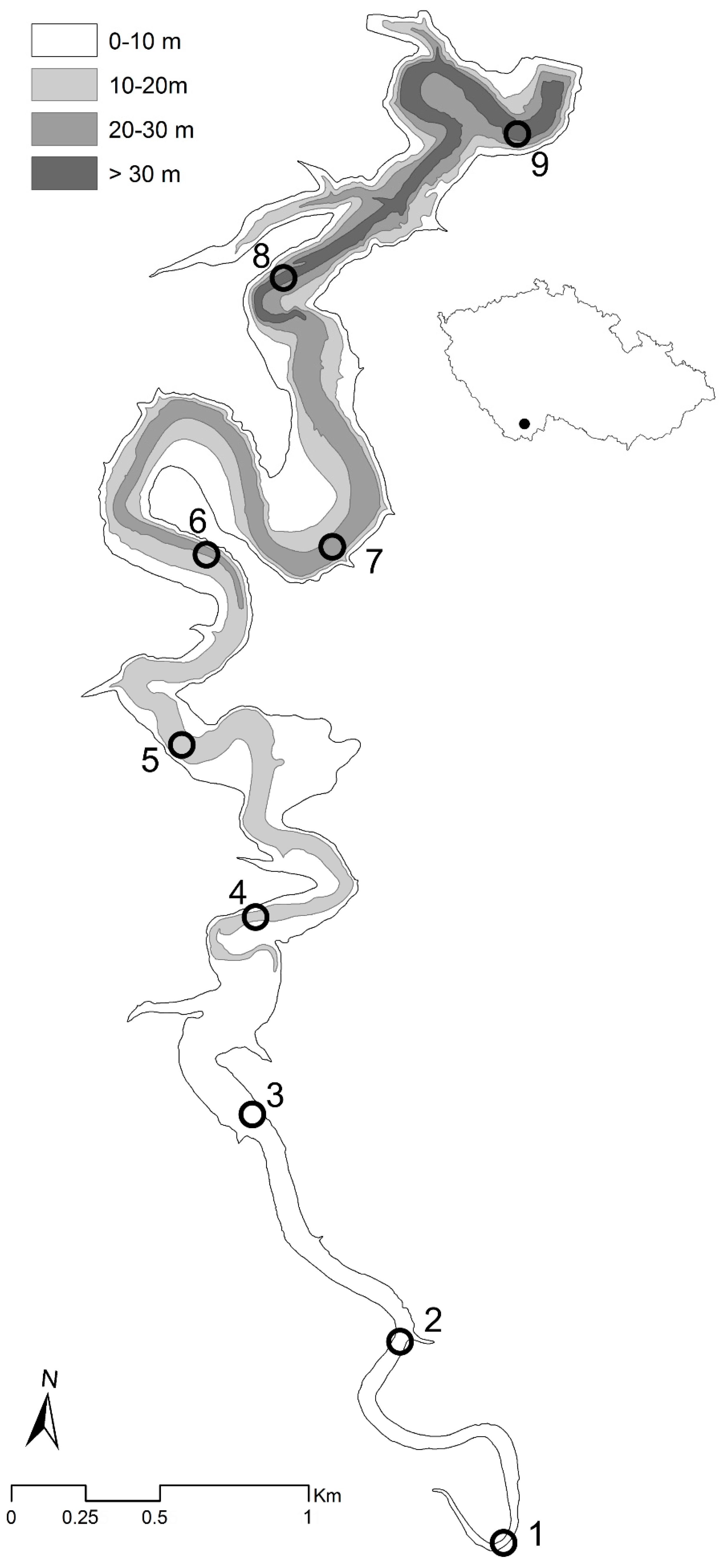
2.1. Study Area Description

The Římov Reservoir (48°50′56″ N, 14°29′26″ E, 471 m above sea level) is a dimictic, deep-valley, 13-km-long reservoir located in the Czech Republic, which was built in 1974–1979 to accumulate drinking water. River Malše is the primary tributary and supplies 90% of the inflow at the long-term average annual flow rate of 4.4 m³/s. It is a small canyon-shaped water body with an area of 2.1 km² and a volume of 33.8 million m³, a maximum depth of 42 m, an average depth of 16 m, and a mean water retention time of 77 days [11]. The reservoir is meso-eutrophic, with pronounced longitudinal gradients in biological and chemical parameters [9,12,13]. The reservoir catchment has an area of 488 km² and a moderately hilly relief, and it is covered primarily by forests, while agricultural land use is relatively limited. The reservoir belongs to the Long-Term Ecosystem Research (LTER) network and is the subject of long-term monitoring of water parameters, fish, and other data during the last 20+ years [14].

2.2. Water-Quality Parameters

The analyses carried out in this work were based on a large dataset of water-quality parameters measured in 2008–2017, primarily between May to November (Table S1 in Supplementary Materials). The measurements were taken at nine sites located along the reservoir’s longitudinal axis (Figure 2). At each site, vertical profiles of water temperature (°C), chl-a, green algae, cyanobacteria, and yellow substance concentrations were measured (in μg/L), using a submersible fluorescence probe (FluoroProbe, bbe-Moldaence, Kiel, Germany) [11]. According to the specific fluorescence spectra of distinct groups of phytoplankton, the probe permits differentiation of Cyanobacteria, Chromophytes + Dinoflagellates (a mixed group with diatoms, frequently being the most important), Cryptophytes, and Chlorophytes in mixed natural populations [15]. The fluorescence probe was provided with original software (FluoroProbe 1.8.4, bbe Moldaence), which allowed the quantification of each phytoplankton group expressed in terms of the equivalent amount of chlorophyll-a per liter of water, and the concentration of yellow substance (relative fluorescence units), which is used as a proxy the amount of colored dissolved organic matter in water. At the site numbers 4, 7, and 9 (Figure 2), vertical profiles of the photosynthetically active radiation were obtained using a LICOR LI-1400 datalogger with a spherical quantum underwater sensor LI 193 SA (LI-COR, Lincoln, NE, USA). At these sites, the euphotic zone depth (Z_eu) was calculated as a depth of 1% of surface irradiance. At the rest of the sites, Z_eu was linearly interpolated as a distance-weighted average of the calculated values of the closest sites, where the data were available. For the purpose of the study, only the mean values of each parameter calculated for Z_eu (not for the whole water column) were used.

2.3. Collection and Processing of Hydroacoustic Data

Acoustic daytime data from July to August between 2008 and 2017 (Table S2) were used to determine the fish distribution along the reservoir. All acoustic surveys were performed in a zigzag pattern with a 120-kHz horizontally aimed transducer (ES120-4 × 10 or ES120 7C) controlled by a SIMRAD EK60 split-beam echosounder. The whole system was calibrated using a 33.2 mm tungsten-carbide sphere [16] and connected to a global positioning system (GPS), using a handheld Garmin GPSMAP 60CSx GPS receiver (GPS accuracy position <10 m) with an external antenna for better reception of the signal (GPS accuracy position <3–5 m).

All the acoustic data were evaluated using the Sonar5-Pro software (CageEye, Oslo, Norway). The raw data were first converted into echograms according to parameters of the latest calibration event of the year. Single echoes were conventionally defined by the echo length 0.6–1.5 with a minimum acoustic target strength (TS) of −70 dB in a 3-dB one-way beam. After detecting single echoes, all targets from a range of 4 to 24 m off the research vessel were automatically tracked to contain at least 3 to 4 single echoes without any gap with gating 0.10–0.15 m. Automatically prepared data were visually scrutinized and manually corrected for inaccuracy or errors induced by automatic approaches and for any object not corresponding to a target of interest. Fish biomass was calculated using the S_V/TS scaling method based on the size distribution of the tracked fish. The size distribution was, however, reprocessed by a de-convolution method to correct the body aspect of the observed targets. A conversion of TS to total fish length was performed according to Frouzova et al. (2005) [17]. The investigated water column from the water surface was set to a depth of 4 m with 78-m-long transects on average.

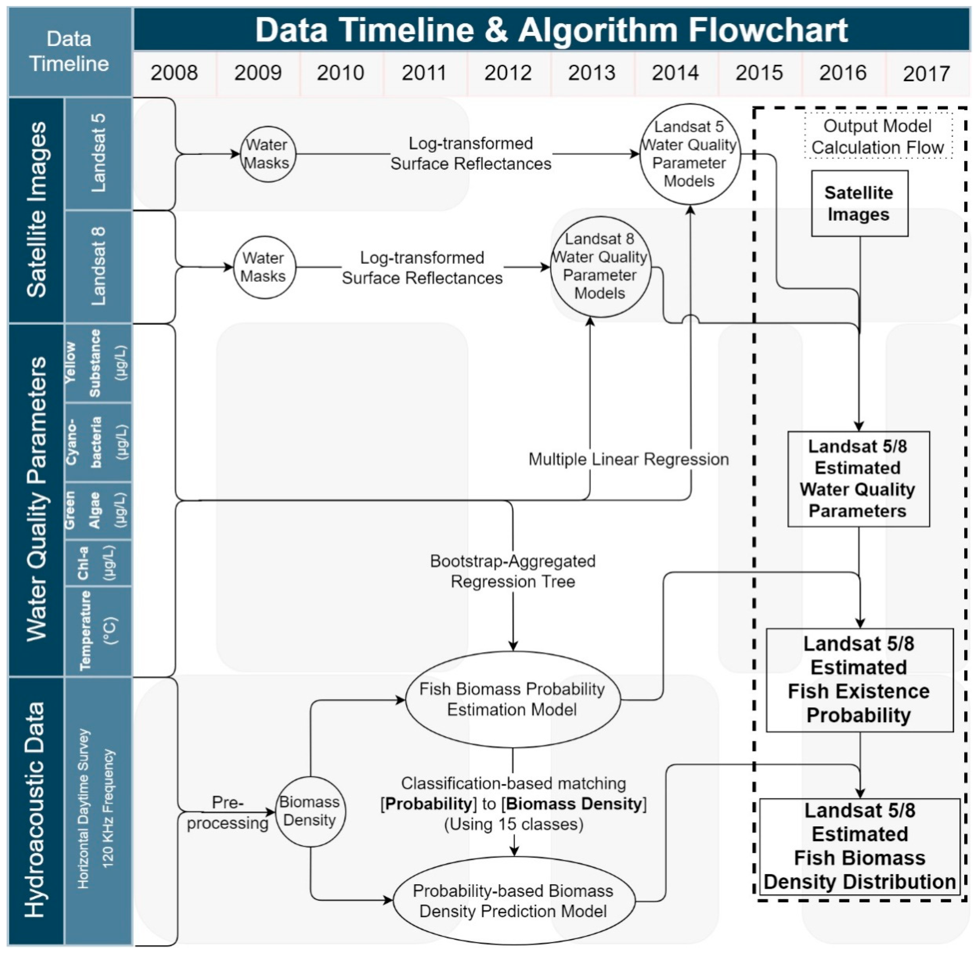
2.4. Satellite Data Mining and Analysis

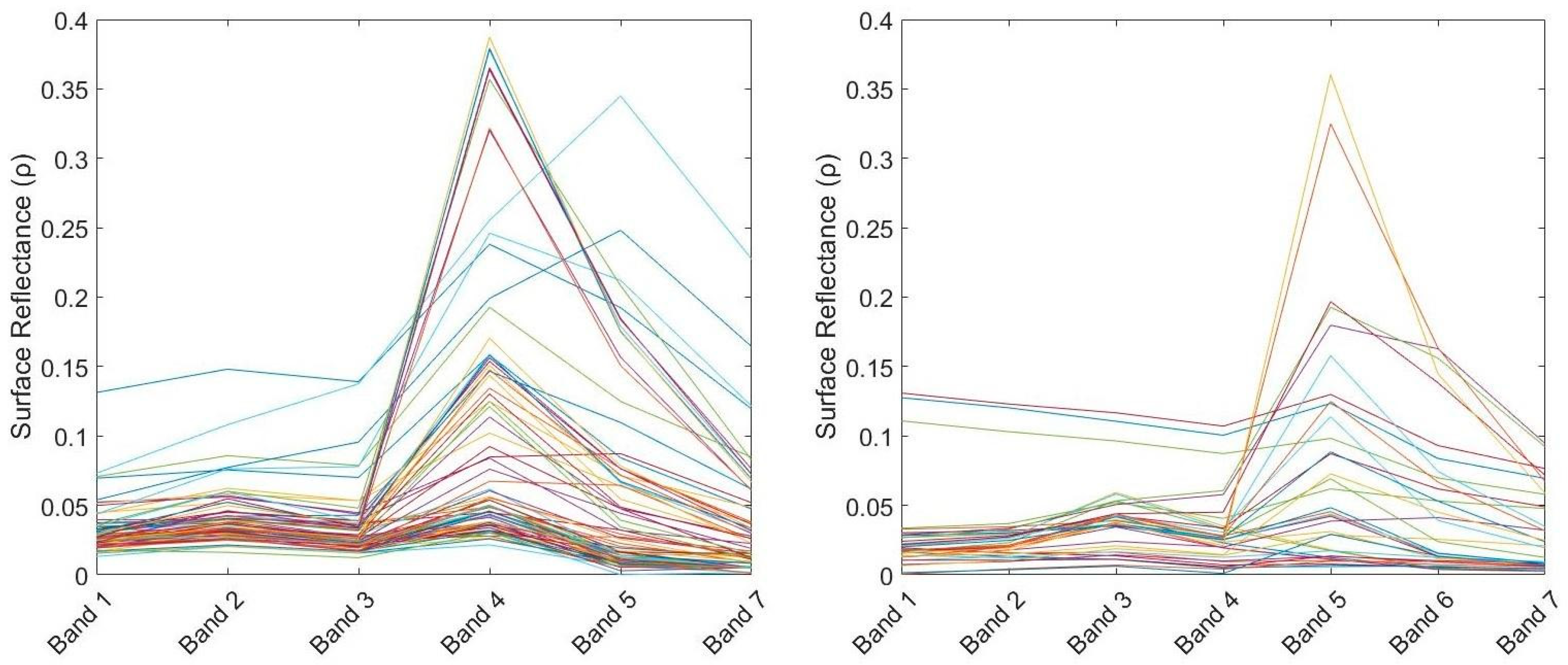
2.4.1. Preprocessing of Satellite Data

The satellite data (Level 2A) of Landsat-5/TM and Landsat-8/TIRS-operation land imager (OLI) -operation land imager (OLI) were used, as these provide the longest consistent time series of space-based surface observations. Typically, only one Landsat scene was required to cover the Římov Reservoir (path/row: 191/26). Appropriate satellite data were identified using Earth Explorer (https://earthexplorer.usgs.gov/). A total of 31 multispectral satellite images were selected (Tables S1 and S2), spanning the period from 2008 to 2017 and fulfilling the following criteria: (a) Less than 70% overall cloud coverage, (b) low cloud coverage over the study area and, especially for water-quality data, (c) availability of water-quality data within a time period of ±10 days from the image acquisition date [18].

“Level 2A Surface Reflectance Products” were ordered and obtained through the Earth Explorer, including all Landsat 5 and Landsat 8 bands necessary for the analysis, except for the thermal bands, which were extracted from “Level 1C products” in the same date points. These were used to estimate temperature by applying the calibration methods described in [19,20].

Surface reflectance products are distributed as georeferenced images with encoded DN values (digital number) for each pixel. DN values were converted to surface reflectance using the appropriate scale factor contained in the product metadata and the resulting images were cropped to a 200 × 129-pixel area of interest (AOI) encompassing the studied reservoir. The AOI geographic extent is defined as [460155 < X (m) < 464025]–[5405385 < Y (m) < 5411385] in the WGS84/UTM Zone 33N Projection (EPSG ID Code: 32633). The Level 2A Products are accompanied by pixel quality assessment bands containing an estimated pixel coverage type classification along with estimation confidence levels. These bands were used to create cloud and cloud shadow masks in order to exclude pixels from the subsequent calculations. Also, water masks for the AOI images were created, isolating pixels covered by water. These water masks and cloud/cloud-shadow masks were utilized at various processing stages depending on processing needs. The output of the preprocessing would be atmospheric and geometric corrected satellite images, cropped at the AOI that will be used for the development of the water-quality models.

2.4.2. Development of Water-Quality Models

To develop water-quality models, the coordinates of all sampling sites were converted into pixel coordinates in the defined AOI. Surface reflectance and temperature values were extracted from the preprocessed bands for each image for all sampling site pixels with a pixel class type of water and not cloud or cloud shadow, based on the accompanying pixel quality assessment bands. Based on standard spectral signatures of water (see e.g., [21]), it was observed that the sampling sites are often located on pixels that do not include water surface, with the strongest indication being the strong reflectance in the near-infrared bands (Band 4 for Landsat 5 and Band 5 for Landsat 8, respectively). These measurements were thus excluded from the analysis if their location was determined to be on pixels located at a distance less than 2 pixels away from the edge of the corresponding water mask.

For each satellite image, the corresponding sampling-date data subset was extracted and parameter values for chl-a, temperature, yellow substance (colored dissolved organic matter), green algae, and cyanobacteria were averaged for the euphotic zone. Temperature values were compared directly, but for the rest of the parameters, combinations of the surface reflectance values were calculated and tested for suitability based on algorithms and statistical models referenced in the literature (e.g., [22,23,24,25]). Parameters were log-transformed [22,23] for most of the models, along with the corresponding band surface reflectance values, unless a better fitting model could be calculated using the original values. Models were tested by multiple linear regression using various bands. After accounting for outliers per parameter case, the models with the highest coefficient of determination (R²) were considered. The selected model can be used to interpolate water quality parameter values over the area of the reservoir based on Landsat 5 and Landsat 8 surface reflectance values.

2.4.3. Fish Spatial Distribution Modeling

To compare fish spatial distribution with water-quality parameters, the selected models were used to estimate the water-quality parameter values in preprocessed satellite images with acquisition dates close to the acoustic survey dates (Table S2). Hydroacoustic data from field surveys were used to model the relationship between water-quality parameters and fish biomass spatial distribution. Acoustic fish biomass values per surveyed transect were mapped to corresponding satellite image pixels based on simultaneous GPS measurements performed during the surveys. Landsat 5 and Landsat 8 data were analyzed separately.

For each pixel, fish biomass was paired with modelled water-quality parameter values at the same pixel and the resulting pairs were analyzed using bootstrapping-aggregated (“bagged”) regression tree ensembles. Bagged regression trees differ from plain regression trees in that they avoid the tendency of plain decision/regression trees to overfit on a training dataset by combining multiple regression trees, each including a different random subset of the observations (bootstrapping), in order to enhance the model generalization capability [26]. Fish biomass was set as the response variable with water-quality parameters as the predictor variables. One image from the Landsat 5 and one from the Landsat 8 fitting datasets were excluded from the analysis, in order to be used as the validation dataset. Bagged-tree performance was assessed for accuracy using out-of-bag error and overall median quantile error, as well as independently against the validation dataset.

Because of potential autocorrelations in the response variable, as well as correlations between the predictor variables, the χ² automatic interaction detection (CHAID) test combined with the curvature test was employed as the split predictor selection methods. The minimum tree leaf size was set to 1 and a set of 100 trees were grown for each of the Landsat 5 and Landsat 8 datasets. This aimed at minimizing the out-of-bag error prior to algorithm truncation. Significance of the predictor variables for each of the Landsat 5 and Landsat 8 models was quantified through permutation-based out-of-bag predictor importance estimates.

The final predictions of the aggregated regression tree model were normalized to [0,1] and interpreted as fish-existence probability values. In order to validate the methodology, fish-existence probability predictions were recalculated using the model.

The estimated probabilities were paired with biomass values from the corresponding processed hydroacoustic datasets for all within-mask pixels. Biomass density–probability value pairs were grouped into classes based on their probability value, and the datasets were analyzed with respect to the average observed biomass per probability class. To facilitate visual interpretation, biomass density was converted and used in the calculations and results as kg per pixel, i.e., kg per 900 m² (from the approximate 30 × 30 m standard pixel dimension of the typical Landsat bands used in the analysis). That way, the biomass density value over a pixel directly represents the observed biomass.

To evaluate the reliability of the model, surveyed data pixels (biomass density values) were combined with predicted probability values from the corresponding bagged tree ensembles using the water-quality parameters from the corresponding validation satellite images. The observed biomass–probability pairs were classified into three classes (corresponding to low, medium, and high probability) and pixels within each class were averaged for surveyed biomass density value. This coarse classification was performed to evaluate the model’s ability to generalize and capture a general fish distribution pattern.

To extrapolate biomass density values for the entire area of the reservoir from the combination of the surveyed pixels and the predicted probability map for the validation satellite image, a more detailed classification method was used. Observed biomass density values were matched to probability values at the same pixels and were separated in 15 classes. Probability values at unsurveyed pixels were then assigned the biomass density value of the corresponding class they were allocated to, using the classification scheme.

3. Results

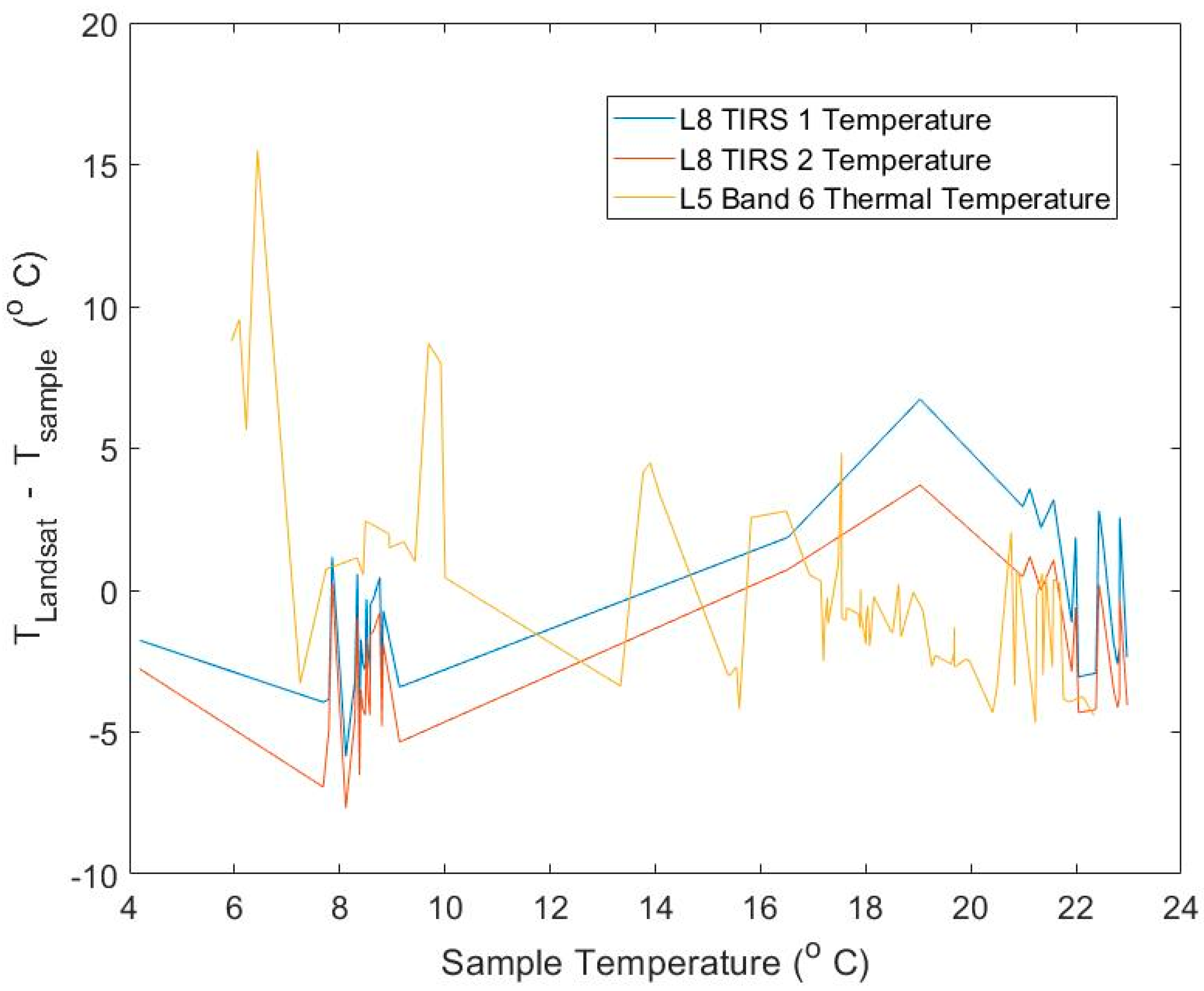
3.1. Development of Water-Quality Models

Due to cloud coverage and lack of in-situ measurements for some satellite image dates, 83 band reflectance–in-situ measurement pairs were assembled for Landsat 5, and 38 pairs for Landsat 8. Figure 3 presents the spectral signatures from obtained reflectance values at the sampling sites. Landsat 5 observations present greater variability in their spectral signatures, which reveals wider fluctuations in land cover in the corresponding pixels. It is also possible that atmospheric variations, as well as the difference in intrinsic sensor accuracy between the two systems, have also played a role in the increased variability that is observed.

Equations (1)–(8) correspond to the models used for the interpolation of water-quality parameter values over the area of the reservoir, based on Landsat-5- or Landsat-8-derived surface reflectance values. Most algorithms are characterized by significant R² values, while the correlations of the water-quality parameters appear to be significant mostly with respect to the visible bands. Chl-a: Chlorophyl-a concentration, CDOM: Colored Dissolved Organic Matter (Yellow Substance), GA: Green Algae concentration, BA: Cyanobacteria concentration.

$$\begin{gathered} \mathrm{LANDSAT}-5: \\ \ln \left(\mathrm{Chl}-a\right)=2.6251+0.533\times \mathrm{lnb}2-0.193\times \mathrm{lnb}4 \\ {\mathrm{R}}^2=0.7507 \end{gathered}$$

(1)

$$\begin{gathered} \mathrm{LANDSAT}-5: \\ \ln \left(\mathrm{CDOM}\right)=0.8987-0.118\times \mathrm{lnb}1-0.138\times \mathrm{lnb}2+0.29937\times \mathrm{lnb}3 \\ {\mathrm{R}}^2=0.8368 \end{gathered}$$

(2)

$$\begin{gathered} \mathrm{LANDSAT}-5: \\ \ln \left(\mathrm{GA}\right)=-1.689-0.396\times \mathrm{lnb}1-0.119\times \mathrm{lnb}5 \\ {\mathrm{R}}^2=0.6928 \end{gathered}$$

(3)

$$\begin{gathered} \mathrm{LANDSAT}-5: \\ \ln \left(\mathrm{BA}\right)=-0.257+19.663\times \mathrm{lnb}1-19.362\times \mathrm{lnb}2+11.557\times \mathrm{lnb}4 \\ {\mathrm{R}}^2=0.8698 \end{gathered}$$

(4)

$$\begin{gathered} \mathrm{LANDSAT}-8: \\ \ln \left(\mathrm{Chl}-\mathrm{a}\right)=4.856-1.821\times \mathrm{lnb}2+2.850\times \mathrm{lnb}3-0.0938\times \mathrm{lnb}4 \\ {\mathrm{R}}^2=0.9417 \end{gathered}$$

(5)

$$\begin{gathered} \mathrm{LANDSAT}-8: \\ \ln \left(\mathrm{CDOM}\right)=-1.016+1.551\times \mathrm{lnb}1-1.990\times \mathrm{lnb}2 \\ {\mathrm{R}}^2=0.9622 \end{gathered}$$

(6)

$$\begin{gathered} \mathrm{LANDSAT}-8: \\ \ln \left(\mathrm{GA}\right)=4.574-1.734\times \mathrm{lnb}2+2.861\times \mathrm{lnb}3 \\ {\mathrm{R}}^2=0.9716 \end{gathered}$$

(7)

$$\begin{gathered} \mathrm{LANDSAT}-8: \\ \mathrm{BA}=-3.803-5.788\times \mathrm{lnb}2+4.951\times \mathrm{lnb}3 \\ {\mathrm{R}}^2=0.9776 \end{gathered}$$

(8)

Thermal bands of Landsat 5 and Landsat 8 were related to in-situ temperature measurements (Figure 4).

It is evident that Landsat 5 thermal bands tend to overestimate low temperatures, whereas it underestimates higher temperatures. At the same time, an increase in estimation accuracy is evident with increasing temperature. The opposite can be seen for Landsat 8. A slight improvement in estimation precision is also evident for Landsat 8-derived temperature reading with increasing temperature.

Because the differences in temperature were significant, a model was best-fitted for them as well. Based on the descriptive statistics of TIRS 1 (sample error: −0.8 ± 2.76 °C) and TIRS 2 (sample error: −2.55 ± 2.54 °C), only TIRS 1 temperature was kept due to the better fit. The estimated models, after maintaining only reflectance-measurement pairs, as well as after exclusion of outliers, were calculated based on linear regression as:

$$\begin{gathered} \mathrm{LANDSAT}-5: \\ {\mathrm{T}}_{{\mathrm{L}}_5}=2.391+0.932\times {\mathrm{T}}_{{\mathrm{b}}_6\left(\mathrm{Thermal}\right)} \\ {\mathrm{R}}^2=0.7986 \end{gathered}$$

(9)

$$\begin{gathered} \mathrm{LANDSAT}-8: \\ {\mathrm{T}}_{{\mathrm{L}}_8}=3.84976+0.800\times {\mathrm{T}}_{{\mathrm{b}}_{10}\left(\mathrm{TIRS}1\right)} \\ {\mathrm{R}}^2=0.9335 \end{gathered}$$

(10)

The algorithms above were used to interpolate the values of the water-quality parameters over the reservoir, based on a water mask extracted from the supplementary pixel quality assessment bands of the retrieved satellite images.

3.2. Spatiotemporal Patterns of Water Quality Parameters

The empirical models were used to estimate water-quality parameters in the period when fish biomass surveys were conducted. To demonstrate the potential of the models for identifying spatial patterns, the spatial distribution was mapped for each parameter for two of the satellite images involved in the fish distribution modelling process. The results were mapped over the area of the reservoir using the corresponding water masks determined from the pixel quality assessment bands (Figures S1 and S2).

In general, the results that are based on Landsat 5 satellite images present a smaller spatial variability than those based on Landsat 8 satellite images. On average, water-quality parameter models for Landsat 5 were fit with a lower overall coefficient of determination than the corresponding models of Landsat 8. Also, Landsat-5-based maps generally appear to span a lower total range for most parameters.

3.3. Fish Spatial Distribution Modelling Results

The descriptive statistics of the training datasets used to develop the bootstrap-aggregated regression tree ensembles can be seen in

Table 1. Descriptive statistics of Landsat 5 regression tree training dataset.

Source Dataset (N = 162)	Mean	Median	Q25%–Q75%	Standard Deviation	Min	Max
Biomass (kg/pixel)	2.227	0.17	0.20–3.01	2.933	0	17.874
Temperature (°C)	21.95	21.94	21.50–22.38	0.4284	21.06	23.25
Green algae (μg/L)	1.32	1.31	1.284–1.1.345	0.057	1.013	1.479
Cyanobacteria (μg/L)	0.087	0.106	0.027–0.116	0.056	0.014	0.0242
Yellow Substance (μg/L)	2.012	2.02	1.961–2.0669	0.066	1.84	2.174
Chl-a (°C)	4.087	4.147	3.918–4.231	0.21	3.682	5.32

and

Table 2. Descriptive statistics of Landsat 8 regression tree training dataset.

Source Dataset (N = 351)	Mean	Median	Q25%–Q75%	Standard Deviation	Min	Max
Biomass (kg/pixel)	2.875	1.368	0.0–1.915	6.355	0	44.477
Temperature (°C)	19.10	19.11	18.96–19.25	0.28	18.4	21.03
Green algae (μg/L)	4.146	3.726	2.721–5.128	1.819	1.9	14.847
Cyanobacteria (μg/L)	6.604	5.516	4.199–8.666	3.66	1.479	34.404
Yellow Substance (μg/L)	1.72	1.739	1.601–1.864	0.191	1.11	2.11
Chl-a (°C)	11.65	10.592	7.918–14.431	4.692	5.497	38.225

, while Figure 5 and Figure 6 depict the out-of-bag error (cumulative MSE error) and the prediction error over the training dataset for the cases of Landsat 5 and Landsat 8 separately. The out-of-bag two-quantile (median) errors (equal to the mean absolute deviations) were calculated to be 0.89 kg/pixel and 1.31 kg/pixel for the Landsat 5 and Landsat 8 trained bagged regression tree ensembles, respectively. Figure 7, Figure 8 and Figure 9 depict the fish-existence probability map, the average biomass-per-pixel probability classes, and the extrapolated biomass distribution maps for Landsat 5 and Landsat 8 modeling cases, respectively. Figure 10 depicts the estimated predictor variable importance for the selected predictor variables, in order of estimated importance. Furthermore, averaging out the extrapolated biomass over the totality of reservoir pixels based on the corresponding water masks, the overall average biomass was calculated, determined to be 16.6 kg/pixel and 10.6 kg/pixel for the Landsat 5 and Landsat 8 validation satellite image, respectively.

Because of the lower variability of the Landsat 5 fish distribution model training dataset, a better fit was calculated based on the model self-calibrated accuracy measures (lower mean squared prediction errors and out-of-bag error). However, external validation revealed a higher reliability of the Landsat-8-based model, as is apparent by interpretation of Figure 8. The Landsat-8-based model appears to better capture the naturally expected trend of pixels with a higher fish-presence probability, also having higher biomass values on average. This trend is not as pronounced in the Landsat-5-based fish distribution model, where pixels with low and medium probability values appear to have the same biomass values on average. However, the Landsat 5 model still clearly exhibits the trend in high fish-presence probability pixels.

Most water-quality-related distribution models exhibit an observable gradient along the reservoir. Due to the nutrient load from the inflow, the upstream part of the reservoir experiences phytoplankton blooms characterized by increases in the concentrations of chlorophyll-a, green algae, and cyanobacteria. Fish presence also appears to be more likely farther from the dam, towards the southern area of the reservoir, although this trend is weaker and even more so for the Landsat-5-based results. The highly dispersed pattern that can be seen in fish biomass distribution maps indicates a higher tendency for localized fish aggregation, rather than extensive assemblage spanning multiple neighboring pixels.

4. Discussion

Our results clearly show that a combination of remote sensing data, earth observation (EO), and hydroacoustic data is a useful tool for detecting spatial trends and constructing prediction models for fish spatial distribution and its relation to water quality in a reservoir. One of the main outputs is shown in Figure 7, which depicts the estimated biomass distribution for the studied dates. The key finding is the observation of a highly heterogeneous fish spatial distribution for these dates. That is in line with similar results of Muška et al. (2018) [8], who observed a patchy fish distribution during daytime. A pronounced difference in detected trends was evident between Landsat-5- and Landsat-8-derived results, as well as between different evaluation dates. In accordance with observations of [4], the usefulness of remote sensing data as auxiliary information for determining fish assemblage patterns is also demonstrated in our study, despite some differences in determined predictor importance for the various parameters, which may be attributed to the differences in satellite systems used, as well as water body morphology and fish composition. The strongest point of the outcome of the present study is the capability of producing dense biomass distribution estimates that depict main distribution trends with a reasonable accuracy, using satellite images. Since satellite imagery is characterized by high-density spatiotemporal availability, the method can provide a low-cost alternative for the monitoring and prediction of biomass distribution. Furthermore, it comprises a fundamental, if not the only, option for past dates of interest, as long as contemporary satellite imagery can be acquired.

While marine waters are a popular target, the use of remote sensing for the monitoring of water-quality, as well as fish distribution, has not been extensively tested in inland waters. A key strength of the present data is the combination of four distinct approaches, namely EO, GIS applications, hydroacoustic surveying, and machine learning. This made it possible to overcome one of the most common problems in modern fisheries research, namely the low spatiotemporal resolution of available data, which precludes conclusive inferences. In the present approach, the availability of multiple heterogeneous data allowed the Římov Reservoir to be used as a case study to test the proposed methodology.

The strengths of the present analysis include the use of data with high spatial resolution, which enables the detection of spatial patterns in fish assemblage in parallel with environmental gradients along the reservoir. Also, despite the localized character of the analysis, the methodologies could be exploited to specialize the design of similar analyses that may focus over specific aspects of water-quality and environmental characteristics of the inland water bodies, and their relations to fish distribution. This can facilitate further investigations of etiologic factors behind the detected trends and outcomes by relevant authorities in the frame of sustainable inland water management.

On the other hand, the most significant limitation of our approach is the incompleteness inherent to all statistical models, namely the inability to capture every potential environmental factor affecting the fish spatial distribution and preferences, as well as the tendency to overstress the significance of the available data (model overfitting). Also, the in-situ dataset used to calibrate the models for water-quality parameter and fish spatial distribution is limited in temporal coverage, spanning the yearly period between early spring to early autumn. Therefore, the output models mirror the specific environmental conditions exhibited during these periods. Application of the models on data outside the seasonal periods, within which the models have been calibrated on, can produce inaccurate results. Furthermore, the exclusion of some measurements for reasons mentioned in the methodology section led to additional gaps in the time-series. Last, but not least, the averaging of in-situ measurements over the Euphotic zone is a design decision with an unforeseeable impact in the final model accuracy, while the determination of the euphotic depth itself was interpolated in most sampling sites, posing an additional potential source of inaccuracy. Finally, because the study was based on past monitoring data, it was not possible to avoid the temporal mismatch between date-of-measurement and corresponding satellite-image dates.

A noteworthy challenge of the present study was the long and narrow canyon shape of the Římov Reservoir. Surface reflectance values, being corrected for atmospheric effects, are affected by spatial autocorrelations due to similar atmospheric conditions over small regions. Because of the small average width of the reservoir, spanning a relatively small number of pixels in the satellite images, these autocorrelations are significant along the entire width. Also, due to the relatively large pixel size (30 × 30 m), reflectance values of pixels close to and across the shoreline are affected by neighboring land covers, while the relatively small spatial resolution leads to a higher degree of generalization for neighboring water pixels. Additionally, the hydroacoustic measurement transects were primarily oriented in the longitudinal (North–South) direction with respect to the main axis of the reservoir. For all these reasons, the ability of the models to detect trends in the transverse direction of the reservoir is significantly weaker than in the longitudinal direction.

An important difference is apparent between variations of parameters over the reservoir as determined from Landsat-5-based and Landsat-8-based results. This might be explained by fundamental differences in sensor resolutions and characteristics, and also because of the significantly different dates (~8 years apart) of the satellite images, based on which the results were developed. Notably, fish composition has changed in the time period spanned by the available data, judging by the fact that the average individual fish length has increased [27]. This, along with other changes in fish composition, also has the potential to lead to such pronounced differences in parameter and fish distribution variance over the reservoir. Another potential explanation might be that the Landsat 5 image acquisition dates for the present case study are very close to the satellite decommission date and natural equipment degradation has affected the collected data quality. Furthermore, improved features of the Landsat 8 OLI (operation land imager) instrument, such as the larger dynamic range and better signal-to-noise ratio [28], can lead to improved spectral resolution and a better capability to model parameter variations.

Mitigating the shortcomings of the methodology as applied in the specific case study can primarily be based on careful planning to best synchronize in-situ sampling, acoustical survey, and satellite imagery acquisition times. Weather is a very important parameter to consider when planning, to also minimize cloud-coverage probability at the dates of sampling. Because much of the in-situ data were sampled at pixels affected by neighboring land cover, it is of utmost importance to design future surveys based on a contemporary satellite image-derived water mask. This is to ensure that sampling is carried out at pixels that are invariably water and sufficiently away from shore pixels, avoiding influence from neighboring non-water land covers. Furthermore, surveying the spectral properties of the water locally, using a portable spectrophotometer in-situ could give insight as to the improvement and calibration of atmospheric correction models, as well as the penetration depth for each wavelength. This could, in turn, help determine suitable sampling depths in order to maximize the correlation between reflectance and sampled parameters. The spatial distribution of the collected hydroacoustic data plays an important part in the determination of the biomass distribution. In order to improve the sensitivity of the model, collecting data in the transverse direction with respect to the reservoir’s primary (longitudinal) axis is a valuable amendment. Additional species composition data from catches could also be included in the analysis. Finally, additional water-quality parameters could also be used to improve and enhance the biomass distribution prediction.

The usefulness of the results for the specific case study of the Římov Reservoir is further hindered by the relatively small water retention time, which leads to a limited temporal validity. This limits the temporal generalizability of the results and necessitates a re-evaluation and recalibration of the models based on the changing nature of the local environmental characteristics, to ensure a consistently up-to-date mapping of the environmental profile and water quality of the reservoir. Finally, it ought to be mentioned that, despite a 30 × 30 m pixel size not being a problem for larger water bodies with more homogeneous environmental parameter distributions, the small total number of pixels covering the Římov Reservoir makes it harder to capture delicate spatial trends spanning smaller extents. As a result, an important future improvement would be the application and re-evaluation of the current methodology using higher-resolution satellite imagery.

References

1. Fox, J.; Nino-Murcia, A. Status of species conservation banking in the United States. Conserv. Biol. 2005, 19, 996–1007. [Google Scholar] [CrossRef]
2. Champ, W.; Kelly, F.L.; King, J.J. The Water Framework Directive: Using fish as a management tool. Biol. Environ. Proc. R. Ir. Acad. 2009, 109, 191–206. [Google Scholar] [CrossRef]
3. Council of the European Parliament. Directive 2000/60/EC of the European Parliament and of the Council of 23 October 2000 establishing a framework for Community action in the field of water policy. Off. J. Eur. Parliam. 2000, 1–72. Available online: https://eur-lex.europa.eu/resource.html?uri=cellar:5c835afb-2ec6-4577-bdf8-756d3d694eeb.0004.02/DOC_1&format=PDF (accessed on 24 October 2019).
4. Sandström, A.; Philipson, P.; Asp, A.; Axenrot, T.; Kinnerbäck, A.; Ragnarsson-Stabo, H.; Holmgren, K. Assessing the potential of remote sensing-derived water quality data to explain variations in fish assemblages and to support fish status assessments in large lakes. Hydrobiologia 2016, 780, 71–84. [Google Scholar] [CrossRef]
5. Stow, D.A.; Hope, A.; McGuire, D.; Verbyla, D.; Gamon, J.; Huemmrich, F.; Houston, S.; Racinef, C.; Sturmg, M.; Tapeh, K.; et al. Remote sensing of vegetation and land-cover change in Arctic tundra ecosystems. Remote Sens. Environ. 2004, 89, 281–308. [Google Scholar] [CrossRef]
6. Lathrop, R.; Lillesand, T.M. Use of Thematic Mapper data to assess water quality in Green Bay and central Lake Michigan. Photogramm. Eng. Remote Sens. 1986, 5, 671–680. [Google Scholar]
7. Noss, R.F. Ecosystems as conservation targets. Trends Ecol. Evol. 1996, 11, 351. [Google Scholar] [CrossRef]
8. Muška, M.; Tušer, M.; Frouzová, J.; Mrkvička, T.; Ricard, D.; Sed’a, J.; Morelli, F.; Kubečka, J. Real-time distribution of pelagic fish: Combining hydroacoustics, GIS and spatial modelling at a fine spatial scale. Sci. Rep. 2018, 8, 5381. [Google Scholar] [CrossRef]
9. Rychtecky, P.; Znachor, P. Spatial heterogeneity and seasonal succession of phytoplankton along the longitudinal gradient in a eutrophic reservoir. Hydrobiologia 2011, 663, 175–186. [Google Scholar] [CrossRef]
10. Znachor, P.; Visocká, V.; Nedoma, J.; Rychtecký, P. Spatial heterogeneity of diatom silicification and growth in a eutrophic reservoir. Freshw. Biol. 2013, 58, 1889–1902. [Google Scholar] [CrossRef]
11. Znachor, P.; Nedoma, J.; Hejzlar, J.; Sed’a, J.; Kopáček, J.; Boukal, D.; Mrkvička, T. Multiple long-term trends and trend reversals dominate environmental conditions in a man-made freshwater reservoir. Sci. Total Environ. 2018, 624, 24–33. [Google Scholar] [CrossRef]
12. Simek, K.; Hornák, K.; Jezbera, J.; Nedoma, J.; Znachor, P.; Hejzlar, J.; Sed’a, J. Spatio-temporal patterns of bacterioplankton production and community composition related to phytoplankton composition and protistan bacterivory in a dam reservoir. Aquat. Microb. Ecol. 2008, 51, 249–262. [Google Scholar] [CrossRef] [Green Version]
13. Vašek, M.; Prchalová, M.; Říha, M.; Blabolil, P.; Čech, M.; Draštík, V.; Peterka, J. Fish community response to the longitudinal environmental gradient in Czech deep-valley reservoirs: Implications for ecological monitoring and management. Ecol. Indic. 2016, 63, 219–230. [Google Scholar] [CrossRef]
14. Znachor, P.; Hejzlar, J.; Vrba, J.; Nedoma, J.; Seďa, J.; Šimek, K.; Komárková, J.; Kopáček, J.; Šorf, M.; Kubečka, J.; et al. Brief History of Long-Term Ecological Research into Aquatic Ecosystems and Their Catchments in the Czech Republic. Part I: Manmade Reservoirs; Institute of Hydrobiology, BC CAS: České Budějovice, Czech Republic, 2016; p. 80. ISBN 978-80-86668-38-3. [Google Scholar]
15. Beutler, M.; Wiltshire, K.H.; Meyer, B.; Moldaenke, C.; Lüring, C.; Meyerhöfer, M.; Hansen, U.-P.; Dau, H. A fluorometric method for the differentiation of algal populations in vivo and in situ. Photosynth. Res. 2002, 72, 39–53. [Google Scholar] [CrossRef] [PubMed]
16. Foote, K.G.; Knudsen, H.P.; Korneliussen, R.J.; Nordbø, P.E.; Røang, K. Postprocessing system for echo sounder data. J. Acoust. Soc. Am. 1991, 90, 37–47. [Google Scholar] [CrossRef]
17. Frouzova, J.; Kubecka, J.; Balk, H.; Frouz, J. Target strength of some European fish species and its dependence on fish body parameters. Fish. Res. 2005, 75, 86–96. [Google Scholar] [CrossRef]
18. Olmanson, L.G.; Bauer, M.E.; Brezonik, P.L. A 20-year Landsat water clarity census of Minnesota’s 10,000 lakes. Remote Sens. Environ. 2008, 112, 4086–4097. [Google Scholar] [CrossRef]
19. Chander, G.; Markham, B. Revised Landsat-5 TM Radiometric Calibration Procedures and Postcalibration Dynamic Ranges. IEEE Trans. Geosci. Remote Sens. 2003, 41, 2674–2677. [Google Scholar] [CrossRef]
20. Zanter, K. Landsat 8 (L8) Data Users Handbook. U.S. Geological Survey, Department of the Interior; Version 1; USGS: Reston, VA, USA, 2015.
21. Jiang, H.; Feng, M.; Zhu, Y.; Lu, N.; Huang, J.; Xiao, T. An automated method for extracting rivers and lakes from Landsat imagery. Remote Sens. 2014, 6, 5067–5089. [Google Scholar] [CrossRef]
22. Tan, W.; Liu, P.; Liu, Y.; Yang, S.; Feng, S. A 30-year assessment of phytoplankton blooms in Erhai Lake using Landsat imagery: 1987 to 2016. Remote Sens. 2017, 9, 1265. [Google Scholar] [CrossRef]
23. Lathrop, R.G.; Lillesand, T.M.; Yandell, B.S. Testing the utility of simple multi-date Thematic Mapper calibration algorithms for monitoring turbid inland waters. Int. J. Remote Sens. 1991, 12, 2045–2063. [Google Scholar] [CrossRef]
24. Matthews, M.W.; Bernard, S.; Winter, K. Remote sensing of cyanobacteria-dominant algal blooms and water quality parameters in Zeekoevlei, a small hypertrophic lake, using MERIS. Remote Sens. Environ. 2010, 114, 2070–2087. [Google Scholar] [CrossRef]
25. Davies-Colley, R.J.; Vant, W.N. Absorption of light by yellow substance in freshwater lakes. Limnol. Oceanogr. 1987, 32, 416–425. [Google Scholar] [CrossRef]
26. Breiman, L. Random Forests. Mach. Learn. 2001, 45, 5–32. [Google Scholar] [CrossRef] [Green Version]
27. Říha, M.; Kubečka, J.; Vašek, M.; Seda, A.J.; Mrkvička, T.; Prchalová, M.; Matēna, J.; Hladík, M.; Čech, M.; Draštík, V.; et al. Long-term development of fish populations in the Římov Reservoir. Fish. Manag. Ecol. 2009, 16, 121–129. [Google Scholar] [CrossRef]
28. Mishra, N.; Helder, D.; Barsi, J.; Markham, B. Continuous calibration improvement in solar reflective bands: Landsat 5 through Landsat 8. Remote Sens. Environ. 2016, 185, 7–15. [Google Scholar] [CrossRef] [Green Version]
Figure 1. Data timeline and algorithmic methodology flowchart. Transparent shading represents data availability per year and dataset, while the dashed line highlights the primary output workflow algorithm, utilizing the individually derived models.
Water 11 02226 g001
Figure 2. A map of the canyon-shaped Římov Reservoir showing location of the sampling stations.
Water 11 02226 g002
Figure 3. Per-band reflectance distributions for all Landsat 5 (left) and 8 (right) satellite-based reflectance observations. As each band captures a very specific wavelength, the graphs approximate the spectral signatures of each sampling site pixel.
Water 11 02226 g003
Figure 4. Satellite-based temperature calculation errors based on sampled temperature values.
Water 11 02226 g004
Figure 5. Cumulative mean squared prediction error for the out-of-bag biomass density values of the training dataset for the Landsat-5-trained regression tree ensemble. Error of prediction on the training dataset observations for the Landsat-5-trained regression tree ensemble.
Water 11 02226 g005
Figure 6. Cumulative mean squared prediction error for the out-of-bag biomass density values of the training dataset for the Landsat-8-trained regression tree ensemble. Error of prediction on the training dataset observations for the Landsat-8-trained regression tree ensemble.
Water 11 02226 g006
Figure 7. Predicted fish biomass distribution map along the reservoir for Landsat 5 validation image (left—29 July 2008) and Landsat 8 validation image (right—20 August 2016).
Water 11 02226 g007
Figure 8. Average biomass density (kg per pixel) per pixel probability class for probability-based pixel classification of Landsat 5 (left) and Landsat 8 (right) validation image.
Water 11 02226 g008
Figure 9. Biomass prediction-based fish occurrence probability map for Landsat 5 validation image (left—29 July 2008) and Landsat 8 validation image (right—20 August 2016).
Water 11 02226 g009
Figure 10. Out-of-bag predictor variable importance estimate for Landsat 5 (left) and Landsat 8 (right) fish biomass distribution model.
Water 11 02226 g010