The Influence of Location on Water Quality Perceptions across a Geographic and Socioeconomic Gradient in Appalachia


School of Natural Resources, West Virginia University, Morgantown, WV 26506, USA
*
Author to whom correspondence should be addressed.
Water 2019, 11(11), 2225; https://doi.org/10.3390/w11112225
Submission received: 27 September 2019
/
Revised: 18 October 2019
/
Accepted: 22 October 2019
/
Published: 25 October 2019
(This article belongs to the Special Issue Integrated Water Resources Research: Advancements in Understanding to Improve Future Sustainability)
Abstract
:Understanding perceptions of water quality held by residents is critical to address gaps in public awareness and knowledge and may provide insight into what defines communities that are more/less resilient to changing water conditions locally. We sought to identify spatial patterns of water quality perceptions gathered in a survey of Southern West Virginia (WV) residents during spring/summer 2018. Using over 500 survey responses across 15 counties, we calculated spatial autocorrelation metrics and modeled the relationships between overall water quality perceptions and county-level socioeconomic endpoints, such as poverty rate, per capita income, and education level. We identified significant differences across counties labeled as socioeconomically “transitional”, “at-risk”, and “distressed”, as it pertained to responses for water quality perceptions, education level, and income level. We also found significant positive relationships between overall water quality perceptions, elevation, and income level. We calculated an empirical semivariogram and fit an exponential model to explain a significant autocorrelation pattern within a range of 104.2 km. Using that semivariance function, we created a kriging interpolation surface across the study area to identify significant clusters of water quality perceptions. This work highlights the influence of location on water quality perceptions within Southern West Virginia, but the analytical framework should be considered in further research, when samples are spread across large areas with varying socioeconomics.
1. Introduction
Water quality may be both broadly and specifically defined across chemical and biological continuums [1]. Endpoints such as pH, conductivity, total dissolved solids, and temperature are often cited as criteria for evaluation of the quality of water and aquatic environments [2,3]. Collection and measurement of water quality information is also a major component used for legal protection of waters of the United States under provisions of the Clean Water Act (CWA) as amended in 1972. Since the passage of the amended CWA, public awareness of water quality has been increasing, with concerns mostly about the physical, chemical, and biological conditions following dramatic crises, such as the Cuyahoga River fire of 1969 [4] or the Exxon Valdez spill in 1989 [5]. Understanding what water quality conditions exist, how they are changing, and how they are perceived or understood is a critical challenge that exists as much today as it has in the past throughout the world.
While the physiochemical endpoints are important for defining water quality as it pertains to the functionality of ecosystems and the services they provide [6], it is also important to define the level of awareness/perception of water quality by people living in a given area. Public awareness and knowledge of local conditions is valuable, as it may help create a sense of place or place attachment which may be linked to social, economic, and environmental benefits [7,8]. Sense of place is a multidimensional concept (person, place, and process) which refers to the way in which a person relates to and perceives the natural environment. People develop a sense of place as they get to know an area, depend on its natural resources, and assign the place meaning and value [9,10]. As a result of this development, a strong sense of place can lead to benefits such as an increase in visitation and economy, social bonding, support for conservation, and the promotion of sustainable uses of natural resources [7,10].
Over time, this can influence a community’s ability to perceive risks and adapt to changes in the quality of their natural resources [11,12]. Communities which are more aware and/or knowledgeable of environmental conditions, such as relative water quality, may be more resilient to changes in resource use, climate, and policy [13]. In contrast, a community largely unaware of resource conditions related to water quality may be more vulnerable to deterioration of water quality and its associated negative health effects [14,15]. This contrast may occur across space, both locally and regionally, which interacts with other important factors, such as income and education, to influence quality of life for residents.
Previous studies have suggested the relevance of socioeconomic and demographic variables in explaining peoples’ perceptions of environmental conditions and how they may respond to environmental issues at both the individual and community level [16,17]. For example, age, income, and length of residency have been significant factors predicting perceptions of water quality and health risks [11,16]. However, a general conclusion about these variables is difficult, as the direction and intensity of their relationship differ from place to place [18]. Research suggests that location of residence and proximity are important in explaining correlations between water quality perceptions and socioeconomic factors [19].
Defining the spatial patterns of public perceptions of water quality requires a baseline understanding of the setting across space and time. For example, within the Appalachian region of the US, a legacy of resource extraction [20], poverty [21], and pollution issues [22] all interact to define the current conditions that residents experience. Within Appalachia, small cities and towns exist, and such areas juxtapose relatively intact forests, rivers, and streams, within some of the oldest mountains on the planet. In particular, Southern West Virginia (WV) has experienced the ebbs and flows of extractive industries from timber harvesting and coal mining, bringing with them both prosperity and fallout [21]. This applies both economically and environmentally, as these industries left behind issues with sedimentation, acid mine drainage, and others which impact water quality. One of the more recent events occurred in January of 2014, when approximately 10,000 gallons of chemicals used to process coal spilled from a storage tank into the Elk River [23]. The Elk River is a primary municipal water source, serving about 300,000 people in the Charleston, WV area. Incidents such as this can have long-lasting impacts on the environment, economy, public health, and well-being. Thus, an understanding of public perceptions is important when it comes to water resource treatment, management, and policy-making. While economic and environmental impacts may be identified and illustrated in distinct units, human perceptions of water quality conditions may operate across more diffuse boundaries which are not strictly defined by census blocks or watershed boundaries [16,17]. Therefore, the main objective of this study was to identify spatial patterns of water quality perceptions in Southern WV as they relate to location and socioeconomic endpoints.
2. Materials and Methods
2.1. Data Collection
In the spring (February–May) and summer (June–August) of 2018, a water quality perceptions survey was created and distributed by West Virginia University (WVU) researchers to 8772 randomly generated addresses within the state of West Virginia, with an emphasis on the southern half of the state. The randomization of addresses was created by random draws from a third-party contractor database, following the methods outlined in a previous study focused on the northern part of West Virginia and water quality perceptions [24]. Surveys have long been used in social science to collect quantitative data from large samples, and they are commonly administered through mail, online, or mixed survey modes [25]. Overall, when mail and online surveys are identical in design and administration method, research has shown no significant differences in response rates or the nature of the data resulting from survey mode [26]. In the present study, both a mail and email version of the survey were distributed to potential respondents, following the methodology outlined by the tailored design method [25]. This method uses personalization and repeated contacts to increase the likelihood that an individual will complete and return the survey. Each study participant was sent a hand-addressed packet of survey materials, which included a cover letter, a survey, and a US postage-paid business-reply envelope [25]. The online survey followed the same schedule. The surveys contained questions related to water quality perceptions, as well as information about the respondents themselves, such as their education and income levels. Location and demographic questions were also included in the survey.
Survey respondents were asked to rate the overall water quality of rivers, streams, and lakes near their home in West Virginia. Responses to overall water quality perceptions were rated on 5-point Likert scale, ranging from “very poor” (1) to “excellent” (5) water quality. Level of education and income were measured as ordinal variables and coded numerically. Location data was collected via coordinates assigned to the IP address on the email/online survey and the self-reported home zip code in the mail-back survey. Locations derived from IP address were also validated by comparing the automatically generated coordinates to the self-reported zip code information in the survey. If the IP address coordinates were not accurate (e.g., different state, far from home zip code, etc.), they were removed from analyses. All completed survey responses were then compiled into a shapefile, within ArcGIS, to be used for spatial analyses. Data used in the analyses are available online and noted as supplementary material to this manuscript.
Data were collected across 15 counties (Table 1) that span across a range of ~150 km in a north-to-south direction and ~230 km in an east-to-west direction. The entire study area represents an area of ~21,000 km2. Mean elevation ranges from 218 m in the western counties to 777 m in the eastern counties. Furthermore, the climate across the study area varies only slightly, with mean annual temperatures in the east ~9.5 °C and the west ~13 °C, and mean annual precipitation ~105 cm in the east and ~109 cm in the west. The eastern counties do receive a much larger mean annual amount of snow (~152 cm) than the western counties (~35 cm), likely due to their higher elevation position in the mountains.
2.2. Data Analysis
Completed surveys with accurate spatial information were also assigned to their respective counties to allow for a county-level comparison of water quality perceptions across those grouped as “transitional”, “at-risk”, and “distressed”. The Appalachian Regional Commission (ARC; https://www.arc.gov/) uses these categories within a multi-metric socioeconomic classification scheme to identify counties which may be vulnerable to high poverty rates, low education level, etc. Counties labeled as “distressed” rank in the bottom 10 percent of all United States counties with respect to index values of unemployment rate, per capita market income, and poverty rate. Counties labeled as “at-risk” and “transitional” rank in the bottom 10–25 percent and the middle 50 percent of all United States counties, respectively. These categories were compared using one-way analysis of variance to identify potential differences in water quality perception scores, and self-reported education and income level scores. In order to evaluate the influence of county on water quality perception scores, we constructed a linear mixed-effects model, using county as a random effect and income, education, distance to 2014 Elk River chemical spill, and elevation as fixed explanatory effects. This model was constructed in package “lme4” [27], within the R statistical environment [28]. The significance of the fixed effects elevation and reported income level was assessed using model comparisons of the full model and a reduced model with each significant variable removed. A likelihood ratio test was then conducted between the full and reduced model to evaluate the significance of the effect of each variable.
Spatial analyses were conducted in both ArcGIS (ESRI, Inc., Redlands, CA, USA), and package “synchrony” [29] within the R environment. We calculated overall spatial autocorrelation in water quality perception scores using Global Moran’s I and used a Getis-Ord General G hotspot analysis to identify areas of high and low water-quality perception score clusters. We then calculated an empirical semivariogram, using the location coordinates. We calculated the significance of the empirical semivariogram, using 999 Monte Carlo randomizations, and compared different semivariance models (i.e., spherical, exponential, etc.), using AIC and root mean square error to select the best fit to the data. Using the best-fitting semivariance model, we created a kriging interpolation surface across the 15-county area to help identify and visualize any significant hot and cold spots of water quality perceptions.
3. Results
3.1. Survey Response and Socioeconomic Analysis
A total of 734 surveys were completed and returned (8.4% response rate overall). The mail-back surveys had a higher response rate (14.1%) than the email surveys (6.7%). Of all the surveys which were completed and returned via either method, a total of 508 (69.2%) surveys were completed with respondents answering the question about the location of their home zip code. Responses were obtained from 15 counties in Southern WV, with a mean of 33.9 ± 1.1 responses per county. The mean (3.0 ± 0.04) overall water quality perception score was scored on a scale of 1–5, with five representing the highest quality and one the lowest quality. The average response came from a resident with a self-reported education level of “some college” and household income of $50,000–$74,999.
West Virginia is the only state entirely within the “Appalachian Region” as defined by the ARC. The ARC criteria for the multi-metric index to classify counties into categories includes three-year mean unemployment rate, per capita market income, and poverty rate (Table 1). These values are then compared for each county to the US national average, to determine what percentile a particular county falls within across the index values. Distressed counties are classified as being the bottom 10% of all US counties. At-risk counties are classified as the lower 10%–25% of all US counties, and transitional counties are classified within 25%–75% of all US counties. Within our 15-county study area, eight counties are classified as distressed, four are at-risk, and three are transitional (Table 1). No counties were classified by the ARC as being competitive or attainment (the two highest performance categories). Across all 15 study counties, mean three-year unemployment rate (8.2% ± 0.6%) is higher than the mean value for WV, the Appalachian Region, and the US (6.5%, 6%, and 5.4%, respectively). The same pattern emerges with respect to study area poverty rate (21.7% ± 1.4%), when compared to the same regional and national averages (17.7%, 16.7%, and 15.1%, respectively). Within the study area, mean per capita income ($19,835 ± $1291) is lower than WV, Appalachian Region, and US means ($25,987, $29,765, and $40,679, respectively).
When comparing the survey response data across county classifications (i.e., distressed, at-risk, and transitional), significant differences exist for overall water quality perception scores (F = 5.67; p < 0.01), with the distressed county group having the lowest mean score (2.84 ± 0.07). Self-reported education and income level differed significantly among county status groups (F = 5.75; p < 0.01; F = 5.49, p < 0.01, respectively), with the distressed county group having the lowest mean score in both response variables (4.5 ± 0.13 and 2.78 ± 0.13, respectively). The linear mixed effects model to describe overall water quality perception scores returned elevation (χ2 = 5.62; p < 0.05) and reported income level (χ2 = 7.92; p < 0.01) as the only significant fixed effects. Both elevation and reported income showed a positive effect on water quality perception score, with elevation showing a slightly stronger effect and income having an effect closer to zero (Table 2). Reported education level and distance from the 2014 Elk River chemical spill were nonsignificant fixed effects. The random effect (intercept) of county only explained 10.2% of the variance in the model following the fixed effects.
3.2. Spatial Analysis
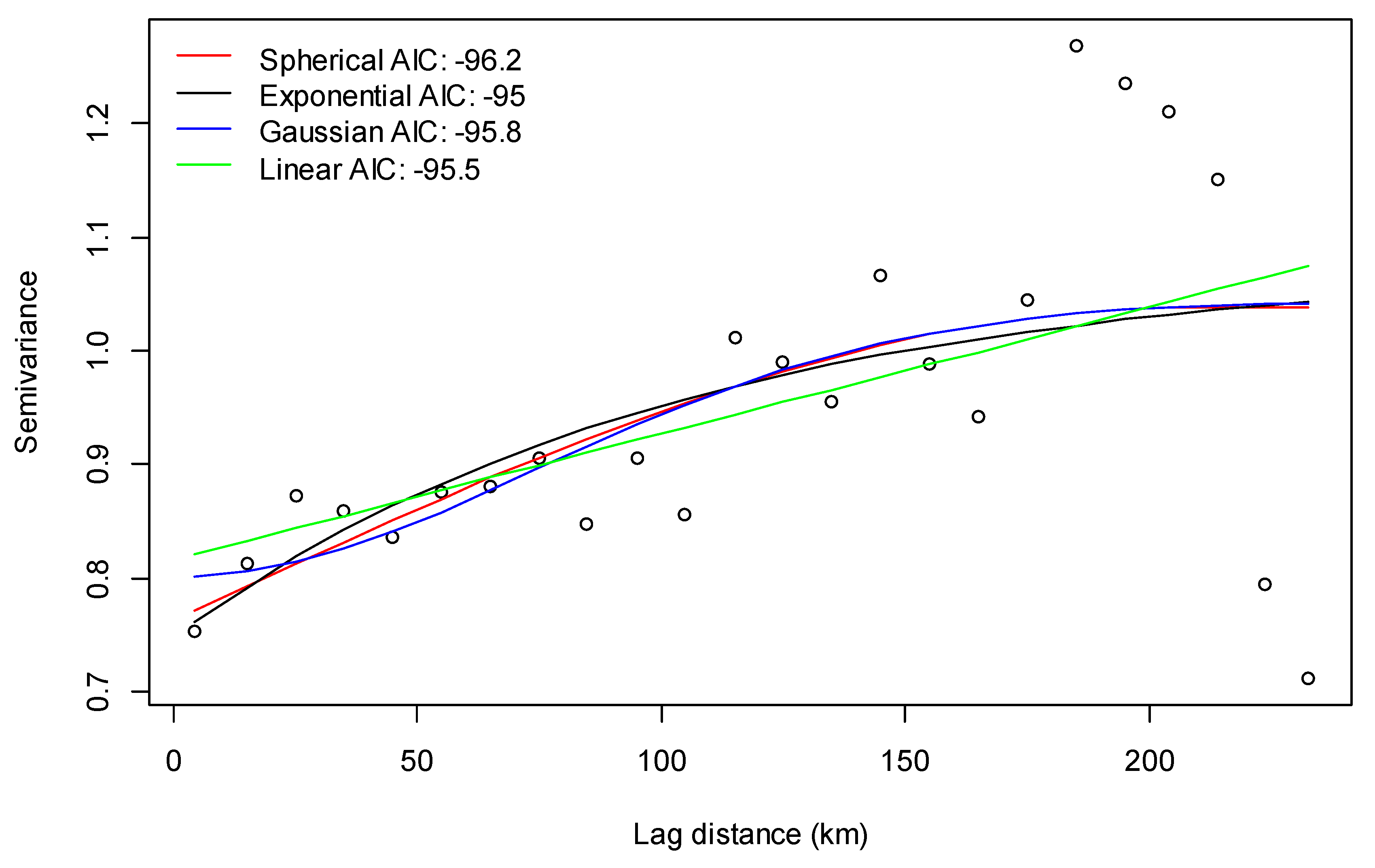
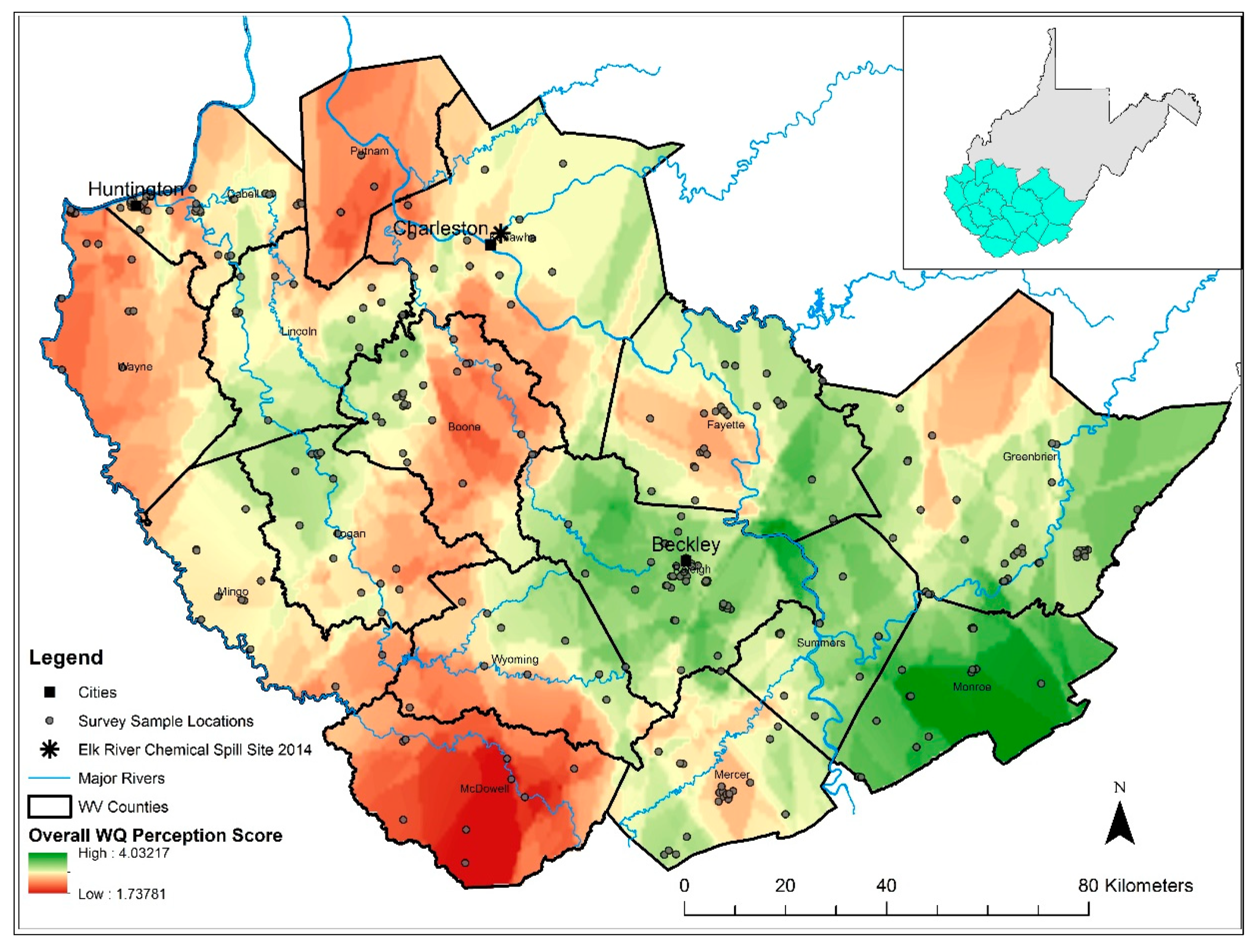
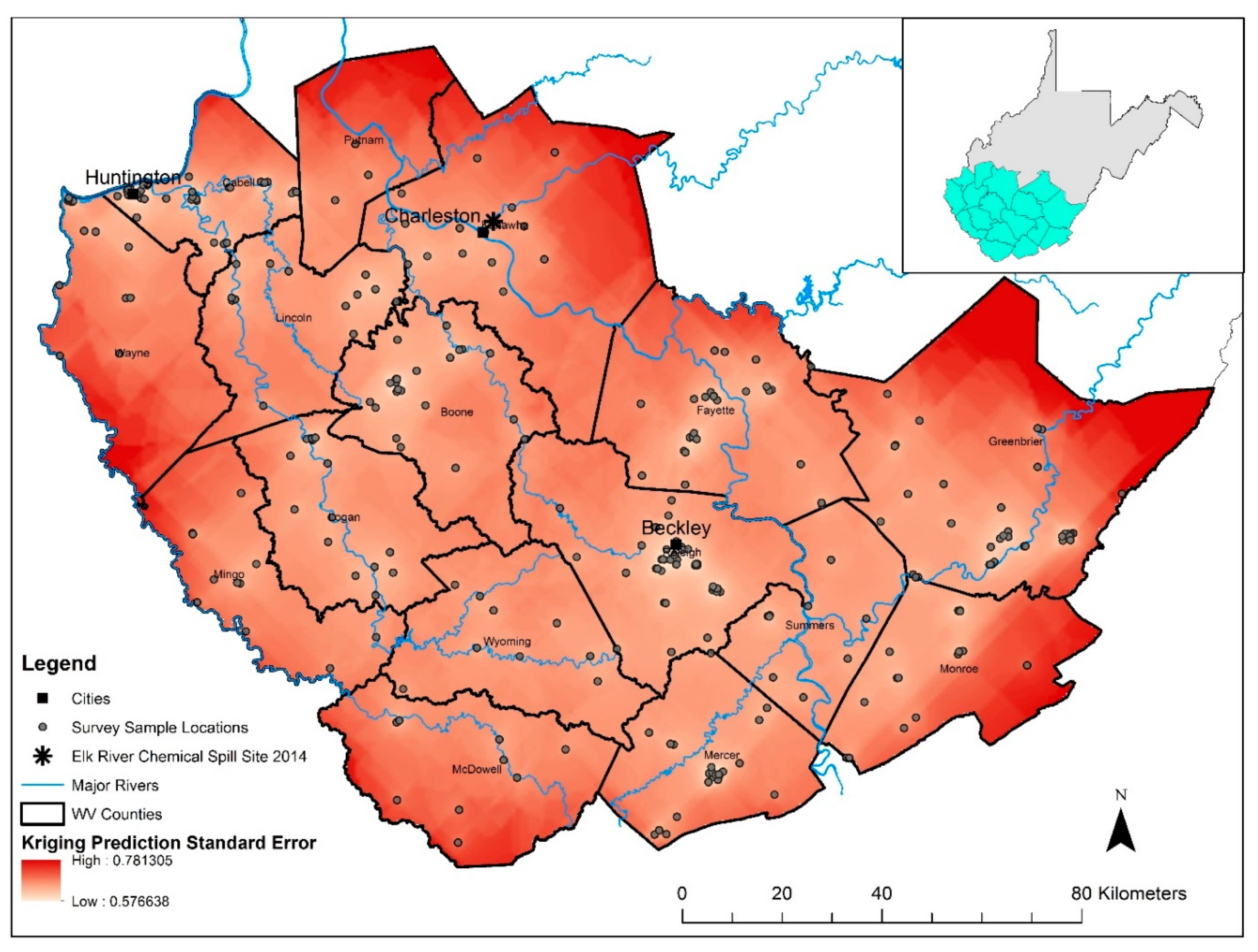
The locational data showed a significantly clustered pattern (Global Moran’s I = 0.04; p < 0.001) with respect to the autocorrelation of water quality perception scores. Furthermore, the high values of these water quality perception scores were more significantly clustered (Getis-Ord General G = 0.52; p = 0.04) than would be expected if the underlying spatial arrangement were random. The empirical semivariogram was fit with four models, each having a somewhat similar AIC and RMSE value. The best-performing model used an exponential semivariance function (RMSE = 0.12; AIC = −95), with maximum likelihood estimates of a range of 104.2 km, nugget = 0.74, and sill = 1.08 (Figure 1). The kriging function produced a prediction surface (Figure 2), with root mean square error = 0.913, mean standardized error = 0.032, root mean square standardized error = 0.986, and average standard error = 0.928. A prediction standard error surface map also indicates relatively low prediction standard error across the majority of the study area (Figure 3).
4. Discussion
Differences in water quality perceptions were identified across socioeconomic status categories for the counties represented in this study. Generally, lower socioeconomic status indicated lower water quality perception scores. This aligns with the socioeconomic status–health gradient, presented originally by Adler et al. to help define how socioeconomic status may interact with and influence disease and mortality in humans [30]. Some meaningful explanatory variables were uncovered in this study with respect to water quality perceptions across space. Specifically, we found income and elevation to have significant relationships with water quality perceptions within our study area. Elevated income may associate positively with environmental concern [31]. Also, income is frequently related to environmental quality experienced, which leads to adverse health conditions and outcomes at the lower levels of income [32]. In central Appalachia, elevated poverty and mortality rates are associated with areas connected to mountaintop coal mining [33], which may also be an underlying factor which influences water quality perceptions and awareness.
Changes in water quality perception across an elevation gradient follows a logical pattern of watershed mechanics along the river continuum. Water quality metrics change as you move downstream, due to both natural and anthropogenic influences [34,35]. From this, water quality perceptions would likely change as you move downstream, as well. Our results indicate this relationship between elevation and water quality perception within West Virginia, which rises in the east to elevations of approximately 1500 m and drops in the west to elevations around 170 m near the Ohio River. Along this elevation gradient, influences from human development, such as mining, agriculture, urbanization, and industrial activities, build cumulatively in a downstream direction. Uncovering the significance of elevation on water quality perceptions is both logical and encouraging, in that residents are somewhat aware of the downstream processes which modify water quality characteristics within the study area.
Both income and elevation were significant in explaining water quality perceptions in this study. The most easily visible spatial gradient within the study area is elevation, moving from east to west in a generally downhill direction. However, in some areas, the influence of socioeconomic factors seems to override or modify the general trend of perception driven by elevation. For example, samples obtained from McDowell County contained an average elevation of 475.1 m. Using the statistical relationship within our model for elevation alone, we would predict an average water quality perception score of around 3.26 within McDowell County. This contrasts greatly with the actual average value of 1.77, indicating a strong influence of the local socioeconomic conditions within the county to lower the water quality perception. McDowell County is a prime example due to its outstandingly low socioeconomic status (<1st percentile nationally for ARC index statistics), but this influence may operate to varying degrees and in both positive and negative directions across the landscape. Inequality of environmental conditions and contamination adjusted by community characteristics of race and poverty level was previously described as a way to define environmental justice, or lack thereof, in some cases [36]. Our findings in McDowell County, in particular, mirror this foundational theory, as lower-income areas tended to have lower water quality perceptions. While the present study does not include data on water quality concerns, lower perception scores could lead to higher levels of environmental concern. For example, residents who have low/poor perceptions of their local water quality would likely view their overall local environmental conditions negatively and thus be more highly concerned about environmental conditions than those living in areas with high/positive perceptions of water quality and the associated environment. This would align with extensions of the environmental justice literature, which indicate higher environmental concern in low-income communities [37] and countries [38] due to the increased risk of exposure to poor conditions.
Surprisingly, education level was not clearly related to water quality perceptions within our study. Higher education level may increase awareness related to water quality and use dynamics [39]. This could be related to our study area, which contains relatively low values of residents with both high school and bachelor’s diplomas. For example, within our study area, 80.2% of residents hold a high school diploma. Within the greater Appalachian region and the entire US, those numbers rise to 85.9% and 87%, respectively. For bachelor’s degree holders, the study area is 14.2%, while the Appalachian region is 23.2%, and the US average is 30.3%. This relatively low level of education across our study area may not allow a wide enough range of educational levels within the surveyed residents to elucidate a relationship between this variable and water quality perceptions.
A notable finding of this study is the lack of a relationship between proximity to the 2014 chemical spill on the Elk River and residents’ overall water quality perceptions. While the spill and the survey samples were separated by four years of time, we suspected lingering effects of public perception within a given distance to the location of the spill site. Time lags between environmental science developments and public perception and understanding have been noted before with more theoretical applications [40]. The chemical spill in January 2014 along the Elk River was declared a State of Emergency by the WV Governor within hours of its discovery, so it is very likely none of our survey respondents were unaware of the event, assuming they were residents of WV in 2014. The lack of a relationship between proximity to the spill site and overall water quality perceptions may indicate a lack of lag time beyond four years for the public perception of water quality in this type of point-source pollution event. Perceptions of environmental concern and water quality have been shown to be influenced by proximity to natural resource extraction activities (i.e., oil and gas wells, and mines) in West Virginia [41]. However, this study showed slight effect sizes across small distances (5 km or less), which contrasts with the spatial extent of the 2014 Elk River chemical spill used in this study.
Spatial analysis of environmental perception data is a useful way to explore and illustrate the potential for coupled relationships of human and environmental systems. Pairing perceptions of environmental quality metrics along with perceptions of human uses of the environment via activities like recreation holds great value for the management of complex settings [42]. Spatial clustering of high and low environmental quality perception values offers insight to locations which may contain tradeoffs for management of environmental conservation and human needs [42]. In the present study, we demonstrate significant spatial clustering of water quality perception values within a region that contains vast potential for tradeoffs between human and environmental coupled systems. For example, high elevation areas hold higher scores for water quality perception but also contain mountains, which produce coal and timber. Therefore, understanding the spatial patterns of these perceptions illustrated in this work can lead to a more holistic view of these settings. Furthermore, spatial analysis of perception score semivariance to elucidate the range of correlation in values using social data holds great promise to examine the range of social autocorrelation across space. While typically used in spatial analysis of environmental variables [29], the application of this technique to social perception data helps define the range of distance at which social perceptions operate. This information is valuable in defining the scale at which coupling of environmental and social systems occurs.
5. Conclusions
In this study, spatial patterns of public perceptions of water quality were illustrated within the context of autocorrelation, as clustering and hot spots of water quality perception scores. Clustering of environmental perceptions is logical, following theoretical constructs of a “sense of place” that emerge to help define people’s relations to their region and environment via social and natural features of their daily lives [43]. Clustering of water quality perceptions may be related to community features that help drive issue-based activism or concern for the health and safety of a localized area [16]. We demonstrate this potential across large spatial areas in Appalachia, with an upper limit of spatial autocorrelation (statistically shown as semivariance range in the variogram) of 104 km. While this distance would not represent a local community as in [16], it may elucidate spatial dependence of environmental perceptions tied to larger regional processes, such as coal mining or agriculture. This finding represents an avenue for further investigation of resident environmental perceptions across space, using more layered and complex suites of covariates. These types of analyses may solidify connections and more closely approximate the reality of socially driven environmental concern and stewardship.
Supplementary Materials
Data used are available at https://github.com/randrew4/spatial-water-quality-perceptions. Please contact the authors for specific information about the survey design and questions used.
Author Contributions
Conceptualization, R.G.A.; methodology, R.G.A. and R.C.B.; formal analysis, R.G.A.; data curation, R.G.A. and R.C.B.; writing—original draft preparation, R.G.A. and M.E.A.; writing—review and editing, R.G.A., R.C.B., and M.E.A.; supervision, R.C.B.; project administration, R.C.B.; funding acquisition, R.C.B.
Funding
This research was funded by US National Science Foundation-Experimental Program to Stimulate Competitive Research (through WV-HEPC-Division of Science and Research) RII Grant: OIA1458952. The APC was funded by the West Virginia University Institute of Water Security and Science.
Acknowledgments
Free and informed consent was asked from participants or their legal representatives and was obtained. The study protocol was approved by the Committee for the Protection of Human Subjects (West Virginia University Institutional Review Board IRB), by West Virginia University, West Virginia, United States, protocol No.1510895135, November 2015. The authors thank two anonymous reviewers and the editorial staff for constructive feedback that resulted in an improved manuscript.
Conflicts of Interest
The authors declare no conflicts of interest. The funders had no role in the design of the study; in the collection, analyses, or interpretation of data; in the writing of the manuscript; or in the decision to publish the results.
References
- Chapman, D. Water Quality Assessments-A Guide to Use of Biota, Sediments and Water in Environmental Monitoring, 2nd ed.; Taylor & Francis: New York, NY, USA, 1996. [Google Scholar]
- Shelton, B.L.R. Field Guide for Collecting and Processing Stream-Water Samples for the National Water-Quality Assessment Program; U.S. Geological Survey Open-File Report 94–455; U.S. Department of the Interior: Sacramento, CA, USA, 1994.
- Bolstad, P.V.; Swank, W.T. Cumulative impacts of landuse on water quality in a southern appalachian watershed. J. Am. Water Resour. Assoc. 1997, 33, 519–533. [Google Scholar] [CrossRef]
- Stradling, D.; Stradling, R. Perceptions of the burning river: Deindustrialization and Cleveland’s Cuyahoga River. Environ. Hist. 2008, 13, 515–535. [Google Scholar] [CrossRef]
- Palinkas, L.A.; Downs, M.A.; Petterson, J.S.; Russell, J. Social, Cultural, and Psychological Impacts of the “Exxon Valdez” Oil Spill. Hum. Organ. 1993, 52, 1–13. [Google Scholar] [CrossRef]
- Keeler, B.L.; Polasky, S.; Brauman, K.A.; Johnson, K.A.; Finlay, J.C.; Neill, A.O. Linking Water Quality and Well-Being for Improved Assessment and Valuation of Ecosystem Services. Proc. Nat. Acad. Sci. 2012, 109, 18619–18624. [Google Scholar] [CrossRef] [PubMed]
- Van Liere, K.D.; Dunlap, R.E. Moral norms and environmental behavior: An application of Schwartz’s norm-activation model to yard burning. J. Appl. Psychol. 1978, 8, 174–188. [Google Scholar]
- Ramkissoon, H.; David, L.; Smith, G.; Weiler, B. Testing the Dimensionality of Place Attachment and Its Relationships with Place Satisfaction and pro-Environmental Behaviours: A Structural Equation Modelling Approach. JTMA 2013, 36, 552–566. [Google Scholar] [CrossRef]
- Williams, D.R.; Patterson, M.E. Environmental psychology: Mapping landscape meanings for ecosystem management. In Integrating Social Sciences and Ecosystem Management: Human Dimensions in Assessment, Policy and Management; Cordell, H.K., Bergstrom, J.C., Eds.; Sagamore: Champaign, IL, USA, 1999; pp. 141–160. [Google Scholar]
- Vaske, J.J.; Kobrin, K.C. Place attachment and environmentally responsible behavior. J. Environ. Ed. 2001, 32, 16–21. [Google Scholar] [CrossRef]
- Boudet, H.; Clarke, C.; Bugden, D.; Maibach, E.; Roser-Renouf, C.; Leiserowitz, A. “Fracking” controversy and communication: Using national survey data to understand public perceptions of hydraulic fracturing. Energy Policy 2014, 65, 57–67. [Google Scholar] [CrossRef]
- Marlon, J.R.; van der Linden, S.; Howe, P.D.; Leiserowitz, A.; Woo, S.L.; Broad, K. Detecting local environmental change: The role of experience in shaping risk judgments about global warming. J. Risk Res. 2018, 22, 936–950. [Google Scholar] [CrossRef]
- Jalan, J.; Somanathan, E.; Chaudhuri, S. Environment and Development Development Economics: Awareness and the Demand for Environmental Quality: Survey Evidence on Drinking Water in Urban India. Environ. Dev. Econ. 2009, 14, 665–692. [Google Scholar] [CrossRef]
- Stern, P.C.; Dietz, T.; Black, J.S. Support for Environmental Protection: The Role of Moral Norms. Popul. Envrion. 1986, 8, 204–222. [Google Scholar] [CrossRef]
- Ekmekçi, M.; Günay, G. Role of Public Awareness in Groundwater Protection. Environ. Geol. 1997, 30, 81–87. [Google Scholar] [CrossRef]
- Brody, S.D.; Highfield, W.; Peck, B.M. Exploring the Mosaic of Perceptions for Water Quality across Watersheds in San Antonio, Texas. Landsc. Urban Plan. 2005, 73, 200–214. [Google Scholar] [CrossRef]
- Hu, Z.; Morton, L.W.; Mahler, R.L. Bottled water: United States consumers and their perceptions of water quality. Int. J. Environ. Res. Public Health 2011, 8, 565–578. [Google Scholar] [CrossRef]
- Wakefield, S.; Elliot, S.J.; Cole, D.C.; Eyles, J.D. Environmental risk and (re)action: Air quality, health, and civic involvement in an urban industrial neighborhood. Health Place 2001, 7, 163–177. [Google Scholar] [CrossRef]
- Syme, G.J.; Williams, K.D. The psychology of drinking water quality: An exploratory study. Water Resour. Res. 1993, 29, 4003–4010. [Google Scholar] [CrossRef]
- Lewis, R.L. Appalachian Restructuring in Historical Perspective: Coal, Culture and Social Change in West Virginia. Urban Stud. 1993, 30, 299–308. [Google Scholar] [CrossRef]
- Partridge, M.D.; Betz, M.R.; Lobao, L. Natural Resource Curse and Poverty in Appalachian America. Am. J. Agric. Econ. 2013, 95, 449–456. [Google Scholar] [CrossRef] [Green Version]
- Bernhardt, E.S.; Lutz, B.D.; King, R.S.; Fay, J.P.; Carter, C.E.; Helton, A.M.; Campagna, D.; Amos, J. How Many Mountains Can We Mine? Assessing the Regional Degradation of Central Appalachian Rivers by Surface Coal Mining. Environ. Sci. Technol. 2012, 46, 8115–8122. [Google Scholar] [CrossRef]
- National Toxicology Program. NTP Research Program on Chemicals Spilled into the Elk River in West Virginia, Final Update. 2016; pp. 1–7. Available online: https://ntp.niehs.nih.gov/ntp/research/areas/wvspill/wv_finalupdate_july2016_508.pdf (accessed on 22 August 2019).
- Levêque, J.G.; Burns, R.C. Predicting water filter and bottled water use in Appalachia: A community-scale case study. J. Water Health 2017, 15, 451–461. [Google Scholar] [CrossRef]
- Dillman, D.A.; Smyth, J.D.; Christian, L.M. Internet, Phone, Mail, and Mixed-Mode Surveys: The Tailored Design Method; John Wiley & Sons: Hoboken, NJ, USA, 2014. [Google Scholar]
- Loomis, D.K.; Paterson, S. A comparison of data collection methods: Mail versus online surveys. J. Leis. Res. 2018, 49, 133–149. [Google Scholar] [CrossRef]
- Bates, D.; Maechler, M.; Bolker, B.; Walker, S. Fitting linear mixed-effects models using lme4. J. Stat. Softw. 2015, 67, 1–48. [Google Scholar] [CrossRef]
- R Core Team. R: A Language and Environment for Statistical Computing; R Foundation for Statistical Computing: Vienna, Austria, 2018; Available online: https://www.R-project.org/ (accessed on 19 March 2019).
- Gouhier, T.C.; Guichard, F. Synchrony: Quantifying variability in space and time. Methods Ecol. Evol. 2014, 5, 524–533. [Google Scholar] [CrossRef]
- Adler, N.E.; Boyce, W.T.; Chesney, M.A.; Folkman, S.; Syme, S.L. Socioeconomic Inequalities in Health: No Easy Solution. JAMA 1993, 269, 3140–3145. [Google Scholar] [CrossRef]
- Scott, D.; Willits, F.K. Environmental Attitudes and Behavior: A Pennsylvania Survey. Environ. Behav. 1994, 26, 239–260. [Google Scholar] [CrossRef]
- Evans, G.W.; Kantrowitz, E. Socioeconomic status and health: The Potential Role of Environmental Risk Exposure. Annu. Rev. Public Health 2002, 23, 303–331. [Google Scholar] [CrossRef]
- Hendryx, M. Poverty and Mortality Disparities in Central Appalachia: Mountaintop Mining and Environmental Justice. J. Health Disparit. Res. Pract. 2011, 4, 44–53. [Google Scholar]
- Chang, H. Spatial Analysis of Water Quality Trends in the Han River Basin, South Korea. Water Res. 2008, 42, 3285–3304. [Google Scholar] [CrossRef]
- Neal, C.; Jarvie, H.P.; Love, A.; Neal, M.; Wickham, H.; Harman, S. Water Quality along a River Continuum Subject to Point and Diffuse Sources. J. Hydrol. 2008, 350, 154–165. [Google Scholar] [CrossRef]
- Bullard, R.D. Dumping in Dixie: Race, Class, and Environmental Quality; Boulder, Color. Westview; Routledge: Abingdon, UK, 1990. [Google Scholar]
- Kurtz, H.E. Scale Frames and Counter-Scale Frames: Constructing the Problem of Environmental Injustice. Political Geogr. 2003, 22, 887–916. [Google Scholar] [CrossRef]
- Fairbrother, M. Rich People, Poor People, and Environmental Concern: Evidence across Nations and Time. Eur. Sociol. Rev. 2013, 29, 910–922. [Google Scholar] [CrossRef]
- Robinson, K.G.; Robinson, C.H.; Hawkins, S.A. Assessment of Public Perception Regarding Wastewater Reuse. Water Sci. Technol. Water Supply 2005, 5, 59–66. [Google Scholar] [CrossRef]
- Ladle, R.J.; Gillson, L. The (Im) balance of Nature: A Public Perception Time-Lag? Public Underst. Sci. 2009, 18, 229–242. [Google Scholar] [CrossRef] [PubMed]
- Levêque, J.G.; Burns, R.C. Water Quality Perceptions and Natural Resources Extraction: A Matter of Geography? J. Environ. Manag. 2019, 234, 379–386. [Google Scholar] [CrossRef] [PubMed]
- Alessa, L.; Kliskey, A.; Brown, G. Social–ecological hotspots mapping: A spatial approach for identifying coupled social–ecological space. Landsc. Urban Plan. 2008, 85, 27–39. [Google Scholar] [CrossRef]
- Cantrill, J.G. The Environmental Self and a Sense of Place: Communication Foundations for Regional Ecosystem Management. J. Appl. Commun. Res. 1998, 26, 301–318. [Google Scholar] [CrossRef]
Figure 1.
Empirical semivariogram plotted as points, with four fitted semivariance models shown as different colored lines. The best-fitting model (RMSE = 0.12) is represented by the exponential curve, with a range of 104.2 km, nugget = 0.74, and sill = 1.08.
Figure 1.
Empirical semivariogram plotted as points, with four fitted semivariance models shown as different colored lines. The best-fitting model (RMSE = 0.12) is represented by the exponential curve, with a range of 104.2 km, nugget = 0.74, and sill = 1.08.

Figure 2.
Kriging interpolated prediction surface using exponential semivariance model to predict overall water quality perception scores across study area in Southern West Virginia. Values range from 1 (lowest water quality perception; red) to 5 (highest water quality perception; green).
Figure 2.
Kriging interpolated prediction surface using exponential semivariance model to predict overall water quality perception scores across study area in Southern West Virginia. Values range from 1 (lowest water quality perception; red) to 5 (highest water quality perception; green).

Figure 3.
Kriging interpolated prediction surface standard error for overall water quality perception scores across study area in Southern West Virginia. Values range from 0.57 (lighter colors) to 0.78 (dark red) across the study area.
Figure 3.
Kriging interpolated prediction surface standard error for overall water quality perception scores across study area in Southern West Virginia. Values range from 0.57 (lighter colors) to 0.78 (dark red) across the study area.


Table 1.
Study area elevation and socioeconomic statistics summarized by county. The random intercept for each county-level water quality perception score is also provided for reference to the mixed-model framework.
Table 1.
Study area elevation and socioeconomic statistics summarized by county. The random intercept for each county-level water quality perception score is also provided for reference to the mixed-model framework.
| County | Overall Mean WQ Perception Score | WQ Perception Score Random Effect Intercept | Mean Elevation (m) | ARC Economic Status | Unemployment Rate 2014–2016 (%) | Per Capita Income 2016 ($ USD) | Poverty Rate 2012–2016 (%) | High School Diploma 2012–2016 (%) | Bachelor’s Degree 2012–2016 (%) |
|---|---|---|---|---|---|---|---|---|---|
| Boone | 2.64 | 2.68 | 268.3 | Distressed | 9.3 | 19,098 | 26.0 | 79.2 | 8.7 |
| Cabell | 2.73 | 2.78 | 218.7 | Transitional | 5.2 | 27,563 | 21.8 | 87.0 | 26.1 |
| Fayette | 3.05 | 2.82 | 563.1 | Distressed | 8.3 | 18,149 | 19.1 | 81.7 | 13.2 |
| Greenbrier | 3.54 | 3.22 | 660.4 | Transitional | 6.3 | 22,761 | 18.4 | 83.8 | 19.6 |
| Kanawha | 2.80 | 2.79 | 260.5 | Transitional | 5.8 | 31,941 | 16.0 | 88.0 | 25.2 |
| Lincoln | 3.19 | 3.04 | 239.4 | Distressed | 9.3 | 17,379 | 25.2 | 79.1 | 9.0 |
| Logan | 2.84 | 2.88 | 247.9 | Distressed | 10.7 | 18,737 | 20.2 | 77.7 | 8.9 |
| McDowell | 1.77 | 2.16 | 475.1 | Distressed | 12.7 | 13,282 | 37.6 | 64.9 | 5.2 |
| Mercer | 3.02 | 2.78 | 772.3 | At-Risk | 7.1 | 20,397 | 21.1 | 83.0 | 19.5 |
| Mingo | 2.69 | 2.79 | 302.4 | Distressed | 12.6 | 14,743 | 26.0 | 73.9 | 9.9 |
| Monroe | 3.44 | 3.17 | 610.2 | At-Risk | 5.3 | 18,284 | 17.1 | 81.4 | 13.4 |
| Raleigh | 3.34 | 3.00 | 686.1 | At-Risk | 7.2 | 23,114 | 17.7 | 84.3 | 18.1 |
| Summers | 3.07 | 2.86 | 627.0 | Distressed | 6.8 | 15,025 | 18.4 | 82.8 | 14.8 |
| Wayne | 2.50 | 2.66 | 220.2 | At-Risk | 6.8 | 21,313 | 20.9 | 79.4 | 12.9 |
| Wyoming | 2.88 | 2.81 | 475.1 | Distressed | 9.8 | 15,743 | 20.1 | 77.4 | 8.2 |
| Average | 3.00 | 2.83 | 479.7 | - | 8.21 | 19,835 | 21.71 | 80.24 | 14.18 |
Table 2.
Linear mixed model results for overall water quality perception score as the dependent variable of interest. Note: * p < 0.05; ** p < 0.01.
Table 2.
Linear mixed model results for overall water quality perception score as the dependent variable of interest. Note: * p < 0.05; ** p < 0.01.
| Parameter | Estimate | Lower 95% CI | Upper 95% CI | Random Effect—County (SD) |
|---|---|---|---|---|
| Intercept | 2.828 | 2.685 | 2.972 | 0.30 |
| Elevation * | 0.199 | 0.117 | 0.282 | 0.30 |
| Education | −0.015 | −0.038 | 0.007 | 0.30 |
| Income ** | 0.068 | 0.044 | 0.092 | 0.30 |
| Distance from Elk River Spill Site | −0.065 | −0.136 | 0.007 | 0.30 |
© 2019 by the authors. Licensee MDPI, Basel, Switzerland. This article is an open access article distributed under the terms and conditions of the Creative Commons Attribution (CC BY) license (http://creativecommons.org/licenses/by/4.0/).
Share and Cite
MDPI and ACS Style
Andrew, R.G.; Burns, R.C.; Allen, M.E. The Influence of Location on Water Quality Perceptions across a Geographic and Socioeconomic Gradient in Appalachia. Water 2019, 11, 2225. https://doi.org/10.3390/w11112225
AMA Style
Andrew RG, Burns RC, Allen ME. The Influence of Location on Water Quality Perceptions across a Geographic and Socioeconomic Gradient in Appalachia. Water. 2019; 11(11):2225. https://doi.org/10.3390/w11112225
Chicago/Turabian StyleAndrew, Ross G., Robert C. Burns, and Mary E. Allen. 2019. "The Influence of Location on Water Quality Perceptions across a Geographic and Socioeconomic Gradient in Appalachia" Water 11, no. 11: 2225. https://doi.org/10.3390/w11112225
Note that from the first issue of 2016, this journal uses article numbers instead of page numbers. See further details here.