Dissolved Inorganic Geogenic Phosphorus Load to a Groundwater-Fed Lake: Implications of Terrestrial Phosphorus Cycling by Groundwater

Abstract

The general perception has long been that lake eutrophication is driven by anthropogenic sources of phosphorus (P) and that P is immobile in the subsurface and in aquifers. Combined investigation of the current water and P budgets of a 70 ha lake (Nørresø, Fyn, Denmark) in a clayey till-dominated landscape and of the lake’s Holocene trophic history demonstrates a potential significance of geogenic (natural) groundwater-borne P. Nørresø receives water from nine streams, a groundwater-fed spring located on a small island, and precipitation. The lake loses water by evaporation and via a single outlet. Monthly measurements of stream, spring, and outlet discharge, and of tracers in the form of temperature, δ¹⁸O and δ²H of water, and water chemistry were conducted. The tracers indicated that the lake receives groundwater from an underlying regional confined glaciofluvial sand aquifer via the spring and one of the streams. In addition, the lake receives a direct groundwater input (estimated as the water balance residual) via the lake bed, as supported by the artesian conditions of underlying strata observed in piezometers installed along the lake shore and in wells tapping the regional confined aquifer. The groundwater in the regional confined aquifer was anoxic, ferrous, and contained 4–5 µmol/L dissolved inorganic orthophosphate (DIP). Altogether, the data indicated that groundwater contributes from 64% of the water-borne external DIP loading to the lake, and up to 90% if the DIP concentration of the spring, as representative for the average DIP of the regional confined aquifer, is assigned to the estimated groundwater input. In support, paleolimnological data retrieved from sediment cores indicated that Nørresø was never P-poor, even before the introduction of agriculture at 6000 years before present. Accordingly, groundwater-borne geogenic phosphorus can have an important influence on the trophic state of recipient surface water ecosystems, and groundwater-borne P can be a potentially important component of the terrestrial P cycle.

1. Introduction

Eutrophication poses a major threat to freshwater lake ecosystems worldwide [1,2,3] and is assumed to be particularly controlled by input of phosphorus (P) [4,5]. Identifying the different pathways of P transport within catchments and determining their relative importance is crucial for optimal freshwater ecosystems management [6,7,8,9]. The general perception is that surface and near-surface hydrological pathways are the main transport routes for external P. This is due to the common assumption that P is retained readily in the aquifer sediments by adsorption and metal complex precipitation, predominantly in the oxic zone [10,11,12].

Over the last few decades, however, evidence of groundwater-transported P has increased [7,8,9,13,14,15,16], indicating that P is not necessarily immobilized in aquifers. Furthermore, there has been increasing awareness that P-rich groundwater can play an important role regarding the trophic state of lakes [14,17,18,19] especially for groundwater-fed aquatic systems [8,9,17,18]. Even in cases where groundwater only makes up a minor part of the lake’s annual water budget, it can still control the trophic state of the lake, if the discharging groundwater contains a high concentration of P [6,20,21].

The geochemical environment in the aquifer may play an important role regarding the mobilization of P within the aquifer. Walter [13] found that P was mobile in groundwater in two distinct geochemical environments: (1) In anoxic environments with a high concentration of dissolved ferrous iron, and (2) in suboxic environments where a continued phosphorus loading has filled all available sorption sites. Phosphorus may also be mobile in oxic environments with low iron concentrations or if the iron is immobilized as FeS. This is consistent with the recorded correlation between sediment redox conditions and mobilization of inorganic P, where the main mechanisms responsible for sediment P release is reductive dissolution of Fe-oxides [11,12,22].

In many studies [7,8,9,13,14,15,17,18,19] the source of P in the groundwater, discharging to a lake, is either shown or expected to be anthropogenic, or it remains undetermined whether the P source is natural or anthropogenic. However, total phosphorus (TP) concentrations above the 0.3 µM (10 µg P/L) threshold for oligotrophic freshwater environments [23] have been recorded in deeper, reduced aquifers [8], where P is highly unlikely to be derived from anthropogenic activities. If groundwater from these aquifers discharges into a lake, naturally released (i.e., geogenic) groundwater-borne P may contribute significantly to the trophic state of the lake [24].

The objective of the current study was to investigate whether geogenic groundwater-borne P can be the dominant external contributor of P. This was done by (1) determining the water budget of a Danish lake, Nørresø, (2) investigating the different water-borne external sources of P, and calculating their relative contributions. In order to put the year-long study into a long-term context the results were (3) combined with results of a parallel paleolimnological study.

The internal release of P, which may play an important factor controlling the concentrations of soluble P in the water column [23,25,26], and thus biotic populations during summer blooms, was not included in the present study. Rather, this paper focuses on the identification of the original, external source of the phosphorus now accumulated in the lake and its sediment.

2. Materials and Methods

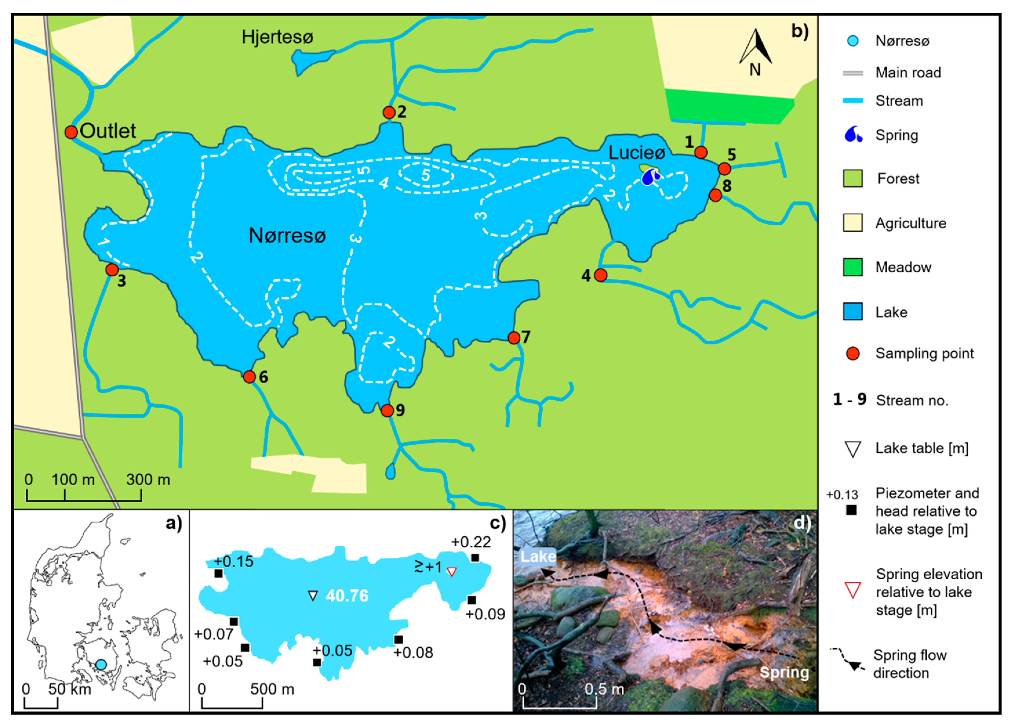
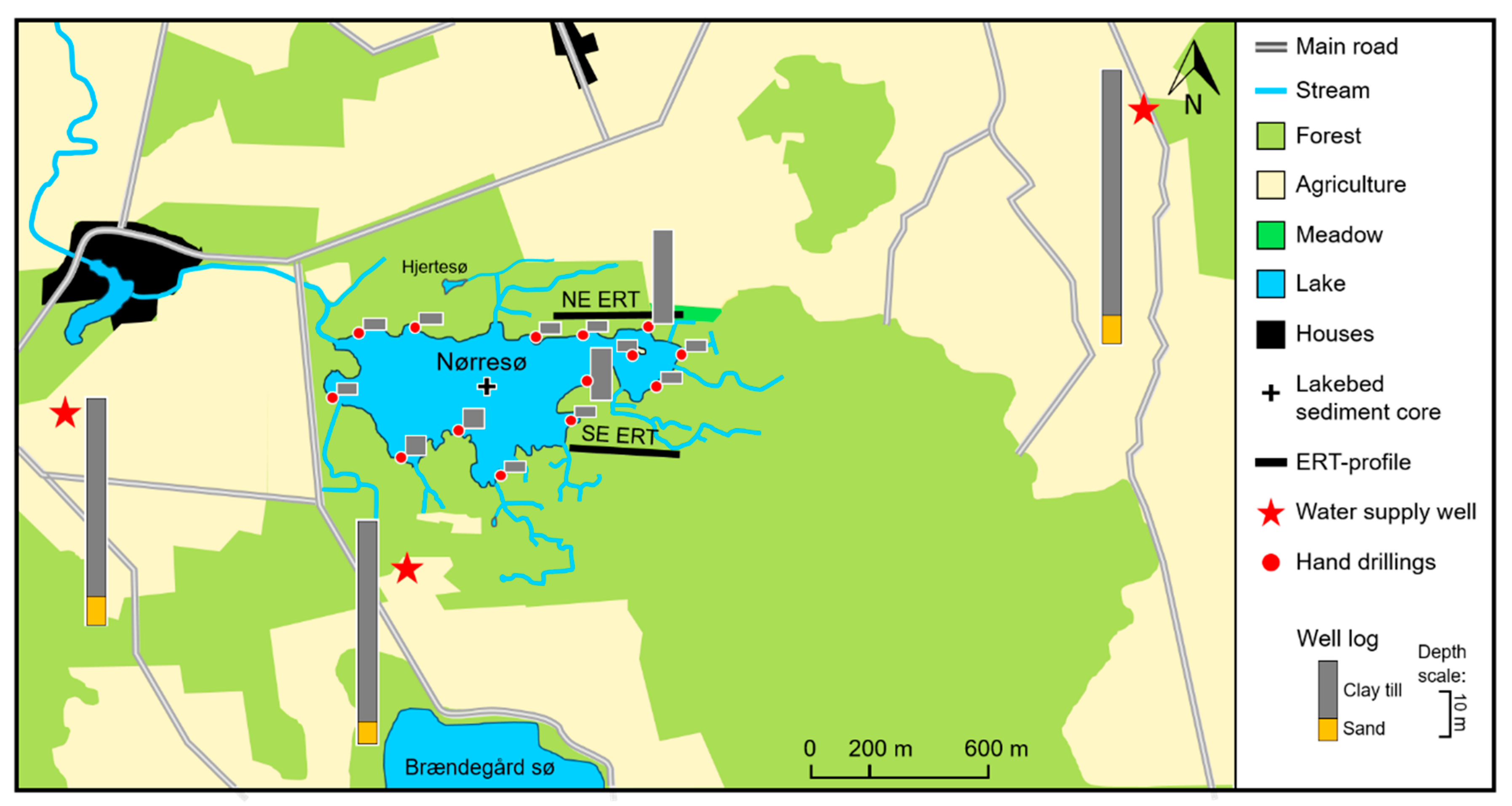
2.1. Study Site

Brahetrolleborg Nørresø (55°08′50″ N, 10°22′40″ E, hereafter for simplicity termed Nørresø) is a lake located in a clay till moraine landscape. The lake formed during the final stage of the Weichselian glaciation [27], in the southwestern part of Fyn, Denmark (Figure 1). Historical maps show that the topographical catchment of Nørresø was dominated by forest through at least the past two centuries [28].

Nørresø is Fyn’s third largest lake, with a geographical surface area of 69.3 ha, including a small island, Lucieø (0.14 ha), located in the eastern end of the lake. The lake has a mean and maximum water depth of 2.3 m and 5.7 m [29], respectively, and the current annual mean elevation of the lake water table is 40.76 ± 0.1 m (seasonal variation) above sea level (ASL).

Visual inflow of water to the lake can be observed from a natural spring elevated 1 m above the lake’s water level, located on the island, Lucieø (Figure 1d). The Lucieø spring is simply referred to as “the spring” in this paper. In addition, nine small streams discharge into the lake. They are, for the purpose of this paper, numbered according to their importance in relation to the determined dissolved inorganic orthophosphate (DIP) loading (kg P/yr), with stream 1 and stream 9 representing, respectively, the highest and the lowest external DIP load. Seven of the streams are ephemeral (Nos. 2 and 4–9), whereas the last two streams (Nos. 1 and 3) and the spring feed water to the lake all year round. The perennial stream 1 receives drainage from a meadow, while the ephemeral stream 2 drains a small lake, Hjertesø, north of Nørresø. Hence the P-loading from stream 2 probably reflects the P-cycling processes within Hjertesø. Just one stream (No. 3) receives water from drainage pipes connected to a large agricultural field located west of Nørresø (Figure 1b). Water is only discharging from the lake via one surface water outlet located at the western end of the lake.

Lake stratification has not been observed in Nørresø [27,29], most likely due to the shallow depth relative to the surface area combined with exposure to westerly winds; the lake is therefore assumed to be a well-mixed lake.

2.2. Data Collection

During a year-long study starting in June 2016 and ending in June 2017, a variety of different methods were applied to investigate the lake, according to the objective of this study. In order to understand the hydrogeology and determine the water budget, four different techniques were used: (1) Observations of lithology (including hand drillings and hydrogeophysics), (2) hydraulic head, (3) discharge measurement (from the outlet, spring, and streams), and (4) a water budget equation (using data obtained through the current study and precipitation and evaporation data extracted from a database). Distinction between streams fed with groundwater from a deep regional confined aquifer as opposed to surface runoff water or groundwater from shallower circulation systems was based on values of δ¹⁸O and δ²H of water combined with the chemical speciation and temperature of the water matrix.

The only bioavailable form of P is orthophosphate (PO₄³⁻), which is the dominant P species in DIP [30]. The focus was, therefore, on the external water-borne DIP loadings. This is further justified as the majority of P entering Nørresø is dissolved inorganic P (cf. [31]). It is, therefore, assumed that TP mainly consisted of DIP and thus the measured DIP concentrations were representative of P entering Nørresø (i.e., particulate P and organic P is of secondary importance; further discussion in Section 4). Quantification of the external DIP loads from the different external water-borne sources were calculated by multiplication of each source’s monthly discharge and associated measured DIP concentration summed over a year. The methods of investigation are further described below.

2.2.1. Lithology

The surficial geology close to the lake shore and on Lucieø was mapped from 13 hand drillings using an Eijkelkamp hand auger and one Geoprobe^® (Salina, Kansas) drilling (see Figure 2 for locations and lithological logs). Eleven of the drillings penetrated to 2 m depth, two went down to 5 m depth, and the Geoprobe^® drilling was 20 m deep. A broader understanding of the geological setting was obtained from lithological logs from three nearby water supply wells (Figure 2) for which data were extracted from the Danish borehole JUPITER-database [32]. The three water supply wells all are less than 3 km from the spring and penetrate down to a confined glaciofluvial sand aquifer (screen depths within 42–58 m below terrain).

In addition, two electrical resistivity tomography (ERT) profiles northeast (NE ERT) and southeast (SE ERT) of the lake, i.e., close to Lucieø (Figure 2) were conducted (Supplementary Materials Section S1 and Figure S1). Interpretation of the inverted data was based on literature resistivity values [33].

2.2.2. Hydraulic Heads

Local interaction between surface water and groundwater can be detected by observations of vertical piezometeric head gradients [34]. Thus, seven piezometers were installed at the lakeshore (Figure 1c) using a pneumatic hammer. They were all placed in clay till and their 10-cm-long screen was installed typically 3 m but up to 12 m below surface. The hydraulic head was measured using a Solinst 101 water level meter or a Solinst 102 coaxial cable fitted with a P4 probe. Elevation of reference points was recorded using a Trimble differential GPS.

The lake water table was measured every 4 hours using two Onset^® pressure transducers with an auto logger function (HOBO Water Level 30′ U20L-01). The pressure transducers were installed at the eastern and western lakeshore. A third similar pressure transducer, installed on land, was used to correct for the atmospheric pressure.

The direction of the underground flow in the confined sand aquifer was estimated based on hydraulic head measurements recorded in the JUPITER-database [32].

2.2.3. Water Budget Equation

A general lake water budget equation can be written in the form [35]:

0 = N + S_in + GW_in − E − S_out − GW_out + ΔSt

(1)

where N is precipitation, S_in is surface water input (stream discharge in streams 1–9), GW_in is groundwater input, E is evaporation, S_out is surface water output, GW_out is groundwater output, and ΔSt denotes storage change.

Groundwater discharge to the lake (GW_in) was divided into two components: Measured groundwater flow (GW_meas) and an estimated groundwater input (GW_est) calculated as the residual of the water balance. GW_meas includes the spring and stream 1. Discussion of this, and other assumptions regarding the water budget components, is presented in Section 4. Precipitation (N) and evaporation (E) values for the catchment were extracted from a database compiled by the Danish National Monitoring Program for Aquatic Environment and Nature [36], where the potential evaporation are quantified based on a modified Makkink equation. The used data are from a 20 × 20 km gridded dataset interpolated from the Danish Metrological Institute’s automated climate stations. The interpolations of potential evaporation for the grid-cell of Nørresø are based on the stations Assens (55°15′ N, 9°53′ E) 32 km WNW of Nørresø, Årslev (55°19′ N, 10°26′ E) 18 km NNE of Nørresø, and Sydfyns Flyveplads (55°01′ N, 10°34′ E) 18 km SE of Nørresø. The climate stations measure hydrological variables every 10 min. The gridded values used for the study were daily averages for the investigated period. Storage change (ΔSt) in the lake was calculated from the average monthly lake water table variation.

2.2.4. Frequency of Collection of Hydrological and Hydrochemical Data

Stream discharge (Q) measurements and water sampling were conducted concurrently on a monthly basis throughout one hydrological year (6 June 2016–21 June 2017) from all streams with a discharge above quantification limit (1 L/min), as well as from the spring and the outlet. Attempts to increase stream discharge measurement frequency via high-frequency monitoring of stream water level (h) using data logger-equipped pressure transducers were unsuccessful. For a successful Q/h-relation to be established, h needs to be controlled by Q. However, water levels in the streams were less affected by stream discharge than by accumulation of leaves and other organic debris in the streams, and by its high-precipitation-event-based removal by flushing or by humans as part of routine stream management.

2.2.5. Outlet, Spring, and Stream Discharge

A cutthroat flume from Baski, Inc. (Englewood, CO, USA) [37,38] equipped with 6.5″ entrance wing walls was used to measure stream discharge of the outlet (S_out; 8″ throat width), and the spring and streams 1–9 (S_in; 1″ throat width).

Triplicate measurements for determination of uncertainty of individual 1″ throat width Baski flume measurements were conducted twice in stream 3, once in stream 5 and once in the spring, at conditions representing nearly the full range of stream flow measurements (not including the outlet), from ~6 L/min (stream 3, June 2017) to 64 L/min (stream 9, December 2016). For each uncertainty determination, measurements were carried out within 30 min at three locations a few meters apart each other along each stream.

The uncertainty expressed as one standard deviation (σ) as a function of the discharge rate (Q) determined by the cutthroat flume was found by linear regression which resulted in the equation σ = 0.157 × Q (r² = 0.99). This equation was then used to determine σ for each specific discharge rate measurement (Figure 6).

2.2.6. Water Sampling and Analysis

All water samples were filtered in the field with 0.22 µm Minisart Sartorius cellulose acetate membrane filters directly into polyethylene vials. Samples for DIP and Fe²⁺ analysis were preserved with 0.1 mL 2 M H₂SO₄ per 5 mL water and ferrozine per 3 mL water, respectively.

Determination of Fe²⁺ and DIP were done spectrophotometrically in the laboratory according to the methods of Stookey [39] and Murphy and Riley [40], respectively. Initially, we also measured the S⁻² concentration. However, none of the samples contained any S⁻², hence sampling for S⁻² was discontinued.

Major cations (Ca²⁺, Mg²⁺, Na⁺, K^+, and NH₄⁺) and anions (F⁻, Cl⁻, Br⁻, NO₃^−, and SO₄²⁻) were analyzed using ion chromatography (IC) and alkalinity was measured by Gran-titration. These analyses were conducted at the hydrogeochemical laboratory at the Section of Geology, University of Copenhagen, Denmark.

The stable isotopes δ¹⁸O and δ²H were analyzed on a Picarro Cavity Ring-Down Spectrometer (CRDS) L2120-i at the Geological Survey of Denmark and Greenland, Copenhagen. Standard deviations were equal to or lower than 0.18‰ for δ¹⁸O and 0.45‰ for δ²H.

DIP, Fe²⁺, O₂, and temperature data of the water matrix in the water supply wells were extracted from the JUPITER-database [32] and assumed representative of the confined aquifer (i.e., representing deep groundwater). Water samples collected from the east and west end of the lake were combined with outlet samples under the term ‘lake’ in the remainder of the paper as the lake is assumed to be well mixed.

Aqueous speciation and saturation index calculations were done using the free software PHREEQC 3.0 developed by David L. Parkhurst and C.A.J. Appelo (United States Geological Survey, Denver, Colorado, USA).

2.2.7. Field Measurements

Measurements of dissolved O₂ were conducted in the field using a WTW oxi-3310 IDS Portable Dissolved Oxygen Meter (accuracy: ±0.5% of value). Values were recorded upon complete stabilization. Temperature was read from the probe. Calibration of the probe was performed in the field in the morning before use. pH and electrical conductivity were measured but are not reported in this paper since there were no significant differences internally between the streams and the spring.

2.2.8. Paleolimnological Analyses

The parallel paleolimnological study conducted within the overall project presents results based on diatom, plant pigment, and pollen analyses of a 6-m-long sediment core section sampled in the center of the lake (Figure 2). These 6 m of the core consist of gyttja accumulated since about 7500 cal yr BP.

The core chronology is based on accelerator mass spectrometry (AMS) radiocarbon dating of terrestrial plant remains (to avoid hard-water effects) found in the Nørresø sediment core. The obtained radiocarbon ages were calibrated to calendar ages (cal yr BP) using IntCal13 [41]. The first obtained ages are presented in this study, while more sediment samples, to allow for a more detailed chronology, are currently being dated.

Elements were analyzed via X-ray fluorescence (XRF) using an ITRAX core scanner (COX Analytical Systems, Mölndal, Sweden). The scanning of the core was performed at the Natural History Museum of Denmark. To normalize the XRF data in order to compensate for the effects of water content, organic matter, and compaction of the sediment through depth, all data were divided with the total scatter (Rhodium incoherent + Rayleigh). A moving average of five neighboring points was calculated for all elements.

Diatom samples were prepared from ca. 0.2 g of freeze-dried sediment, which was prepared following standard methodologies [42]. Briefly, the sediment was oxidized at 90 °C for 6 hours using hydrogen peroxide (H₂O₂, 30%) in order to remove organic material. Carbonates were then dissolved by addition of a few drops of HCl (35%). The test tubes in which samples were treated were subsequently filled with distilled water and left to settle for 12 h. Residues were then washed several times using demineralized water. A few drops of the final suspension were dried on a cover slip and subsequently mounted in Naphrax^® for identification, which was conducted using an optical microscope (Leica DMLB), equipped with phase contrast, at a magnification of ×1000.

Pigments were quantitatively extracted in an acetone:methanol:water (80:15:5) mixture. Extracts were left overnight at −10 °C, filtered with a polytetraflourethylen (PTFE) 0.2 μm filter and dried under nitrogen gas. A known quantity was re-dissolved into an injection solution of a 70:25:5 mixture of (1) acetone, (2) ion-pairing reagent (IPR; 0.75 g of tetra butyl ammonium acetate and 7.7 g of ammonium acetate in 100 mL water), and (3) methanol and injected into a high-performance liquid chromatography (HPLC) unit. Pigment extracts were separated using an Agilent 1200 series separation module with quaternary pump. The mobile phase consisted of solvent A (80:20 methanol: 0.5 M ammonium acetate), solvent B (9:1 acetonitrile: water), and solvent C (ethyl acetate) with the stationary phase consisting of a Thermo Scientific ODS Hypersil (Thermo Fisher Scientific, Waltham, MA, USA) column (205 × 4.6 mm; 5 µm particle size). Eluted pigments passed through a photo-diode array detector and UV-visible spectral characteristics were scanned at between 350 and 750 nm. Quantification was based on scanning peak areas at 435 nm and calibrating to a set of commercial standards (DHI LAB Products, Hørsholm, Denmark). Pigment concentrations are reported as molecular weights of pigments in nanomoles per unit dry weight of sediments.

Samples for pollen analysis were prepared from 1 cm³ of sediment following Faegri & Iversen [43]. Briefly, 37% HCl was used to remove calcium carbonate and samples rinsed 3 times before boiling in a water bath in centrifugal tubes in 10 mL 10% KOH for about 10 min. After rinsing twice with water, 10 mL concentrated HF (40%) was added and the samples boiled in a water bath for 20–25 min. The samples were then centrifuged and rinsed once with 10 mL 10% HCl and once with water, before 10 mL of concentrated acetic acid was added and the samples were rinsed. This was followed by acetolysis. Finally, the samples were suspended in tert-butanol and transferred to a preparation glass. Drops of silicon oil (AK 2000) were added, before placing the samples for evaporation in a heating cabinet at 50 °C for 2 days. Pollen was counted using a light microscope at a magnification of ×400, higher magnification (×1000) was used for identifying taxonomically difficult pollen types. At least 300 terrestrial pollen grains were counted per sample. The pollen sum, which the percentages are based on, includes all terrestrial pollen taxa.

3. Results

3.1. Lithology

In general, the 13 hand drillings all showed two types of sediment: A 0.2–0.7 m thick top layer of peat (not shown in Figure 2) followed by grey clay-rich till (seen in Figure 2). The lower boundary of the till was not detected. The grey color of the till indicated reduced conditions. The same clay till was also found in the 20 m deep Geoprobe^® drilling and in the lithological logs of the three water supply wells. The water supply wells all penetrate a ≥35 m thick layer of clay till which confines a deep anoxic glaciofluvial sand aquifer. Furthermore, clay till was indicated by slow (few months) equilibration of hydraulic pressures in the piezometers screened at up to 12 m below ground. The two ERT profiles (located close to the spring) underlined the occurrence of a thick clay layer (>15 m) confining a sand layer. However, the ERT profiles also indicated that the deep-lying sand layer appears to be connected to the terrain through a thin sloping sand layer (Figure S1 in Supplementary Materials). Hence, the spring could possibly be connected to the deep confined regional aquifer via such sand layers.

3.2. Hydraulic Heads

Groundwater flow in the underlying confined aquifer is toward the southwest. Hydraulic heads in the regional aquifer (42–49 m ASL) were 1–8 m higher than the lake level (40.76 m ASL), resulting in upward hydraulic gradients. The upward gradients were confirmed in all seven of the lakeshore piezometers which had water levels ranging from 0.05–0.22 m above the lake level (Figure 1c).

3.3. Water Samples

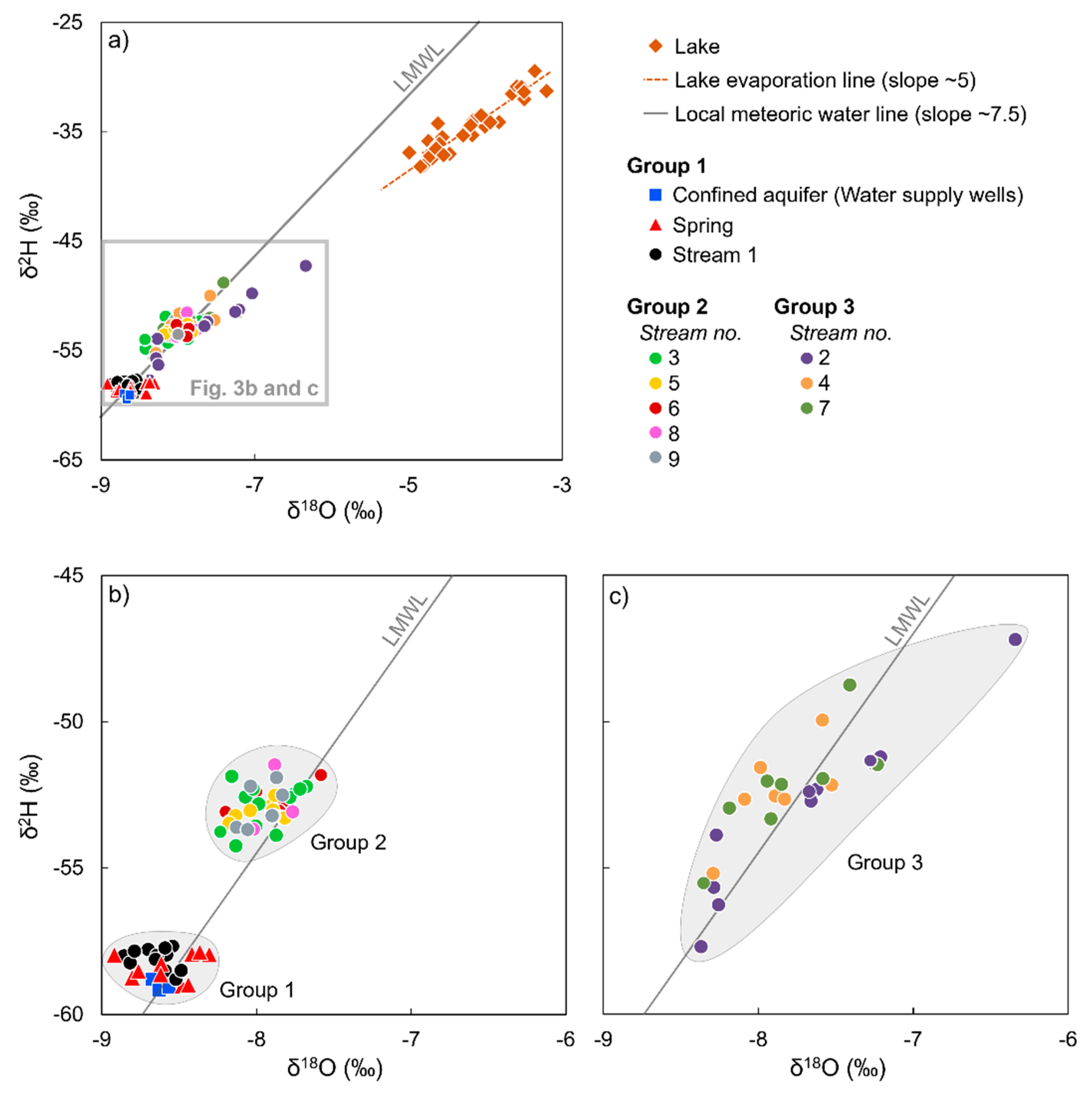
3.3.1. Stable Isotopes of Water

The isotopic composition of the lake differed significantly from that of the streams, the spring, and the confined aquifer. Lake water samples had the most enriched values of δ²H (−38.1‰ to −0.9‰) and δ¹⁸O (−5.0‰ to −3.2‰) as well as the largest seasonal variation (Figure 3a). However, during no season did the lake water isotopic signature overlap with that of the other groups. The isotope data plotted along a line with a distinctly lower slope (~5) than that of the local meteoric water line (LMWL, δ²H = 7.48 × δ¹⁸O + 5.36; [44]). This can be explained by the lake’s relatively long hydraulic retention time of 1.6 years, which enabled evaporation to significantly enrich the isotopic composition.

The nine streams, the spring, and the confined aquifer were subdivided into three groups according to their isotopic composition; the subdivision is shown in Figure 3b,c, which are subsets of Figure 3a. Isotopic group 1 represents the samples where the isotope compositions were almost stable throughout the year. Group 1 consists of stream 1, the spring, and the confined aquifer where the δ²H and δ¹⁸O (mean δ²H = −58.2‰, −58.3‰, and −57.9‰, respectively, mean δ¹⁸O = −8.6‰ for all three) are significantly depleted relative to rest of the streams and clusters within a relatively narrow range (1 std. dev. (σ) for δ²H is 0.3–0.4‰, and 0.2‰ for δ¹⁸O), thus indicating a shared source of water between these three sources. Isotopic group 2 consists of streams 3, 5, 6, 8, and 9. Their isotopic composition lies likewise within a relatively narrow range (σ for δ²H is 0.8–0.9‰, and 0.1–0.3‰ for δ¹⁸O), though isotopically enriched (mean δ²H are −52.7‰, −53.0‰, −52.4‰, −52.9‰, and −52.6‰, respectively, and mean δ¹⁸O is −7.9‰ for all five sources) relative to group 1 (Figure 3b). Isotopic group 3 consists of streams 2, 4, and 7 and represents the three streams with the largest seasonal variation (σ for δ²H is 1.5–2.8‰, and 0.3–0.6‰ for δ¹⁸O).

Stream 2 stands out in particular with signatures ranging from −57.7‰ to −47.2‰ for δ²H and −8.4‰ to −6.3‰ for δ¹⁸O, thus containing the isotopically heaviest water of the streams and spring (Figure 3b,c). The stream 2 data, moreover, plot along a line with a lower slope than the LMWL, indicating an evaporation trend similar to that of the lake water in Nørresø (Figure 3a). This is consistent with stream 2 seasonally getting water from the small lake, Hjertesø (cf. Figure 1b).

The δ-values of isotopic group 1 were significantly different from the δ-values of both groups 2 and 3 with a level of significance of 5%. In contrast, there was no significant difference between the δ-values of isotopic groups 2 and 3.

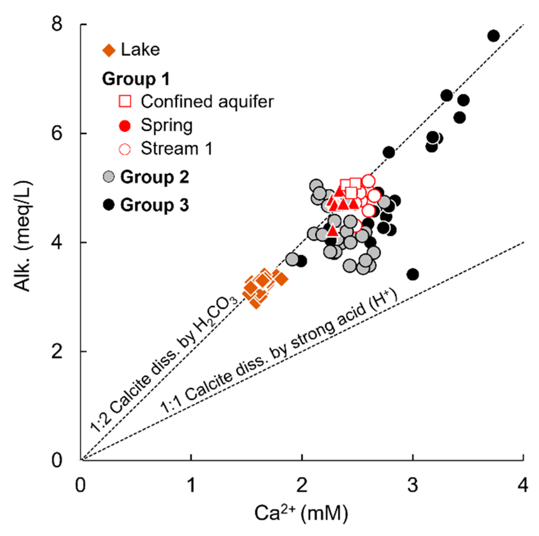
3.3.2. Ca²⁺ and Alkalinity

Ca²⁺ and alkalinity (dominantly bicarbonate, HCO₃⁻) made up >80% of the total charge equivalents in the water compositions in all the streams, the spring, the confined aquifer, and the lake with a molar Ca:HCO₃ stoichiometry for all data close to 1:2 (Figure 4). Accordingly, the process of (calcium) carbonate dissolution by carbonic acid [45] can generally be assumed to control the water chemistry in this freshwater ecosystem.

When measured Ca²⁺ and alkalinity data for the different streams and the spring were grouped with respect to their isotopic grouping (cf. Figure 3), one can see the same trends as for the isotopic composition (Figure 4). Group 1 clustered within a relatively small range, group 2 clustered likewise, however within a larger interval. Group 3 showed a fairly large scatter but the data generally still fall close to the 1:2 line.

3.3.3. Dissolved Inorganic Phosphorus

As compared to the other streams, DIP concentrations measured in the spring and stream 1 were very stable and relatively high (Figure 5a), from 4 to 5 µM (σ of 0.2) in the spring and from 2 to 4 µM (σ of 0.4) in stream 1. The same high DIP concentrations were found in the confined aquifer (mean of 5 µM, n = 4) tapped by the water supply wells. This corresponded to the grouping by similar trends in isotope data where group 1 deviated from the other two groups.

In contrast, there was no correlation between the isotopically determined groups 2 and 3, and the respective streams’ DIP concentrations. Among groups 2 and 3, stream 2 showed the highest and most fluctuating DIP concentrations (σ of 3.4), with values from 2 µM up to as high as 16 µM in December 2016. DIP concentrations in stream 3 were somewhat lower, from 1.3 to 3.6 µM (σ of 0.6). The rest of the streams (Nos. 4–9) all had mean DIP concentrations less the 1.5 µM. The lowest DIP concentrations were measured in streams 5, 7, and 9, with DIP mean concentrations of 0.3 µM.

DIP concentrations in the lake varied throughout the year, from 2 to 12 µM (σ of 2.9). Thus in most months the concentration in the lake was significantly higher than in any of the streams.

3.3.4. Fe²⁺, O₂ and NO₃⁻ Concentrations

The highest concentrations of Fe²⁺ were found in the spring and stream 1 with a mean of 36.5 µM and 23.8 µM, respectively (Figure 5b). Concurrently, low concentrations of O₂ were measured with means of 0.01 mM and 0.09 mM for the spring and stream 1, respectively (Figure 5c). Similar Fe²⁺ (31 µM) and O₂ (<0.008 mM) concentrations were found in the regional confined aquifer. The high concentration of Fe²⁺ and DIP in the aquifer could potentially favor the formation of vivianite [46]. However, according to a PHREEQC speciation (Section 2.2.6), all samples collected in this study were subsaturated with respect to vivianite.

The Fe²⁺ and O₂ concentrations in the spring, stream 1, and the confined aquifer (i.e., group 1) differed significantly from all the other streams (i.e., groups 2 and 3), which showed concentrations of Fe²⁺ generally below 3 µM and concentrations of O₂ much closer to saturation, which was 0.2–0.4 mM, depending on temperature (Figure 5b,c); with the exception of stream 9, in which low concentrations of O₂ were measured (mean of 0.04 mM). Low Fe²⁺ and high O₂ concentrations were likewise measured in the lake water column with means of 0.5 µM Fe²⁺ and 0.3 mM O₂.

The relatively high nitrate concentration in stream 3 (mean: 0.63 mM) differed from all the other streams and the spring (Figure 5d). The lowest nitrate concentrations were recorded in the spring, stream 1, and the confined aquifer (i.e., group 1) with a mean of 0.02 mM. The other streams and the lake all had a mean nitrate concentration in the interval 0.03 to 0.06 mM with the exception of stream 4 (mean: 0.20 mM) and 5 (mean: 0.15 mM).

3.3.5. Temperature

The temperature in the spring and stream 1 was relatively constant at ~9 °C throughout the sampling period, corresponding well to the mean temperature measured in the regional confined aquifer (~9.5 °C). In contrast, temporal variability in temperature from 0 to 20 °C was recorded in all other streams (i.e., groups 2 and 3) and in the lake (Figure 5e).

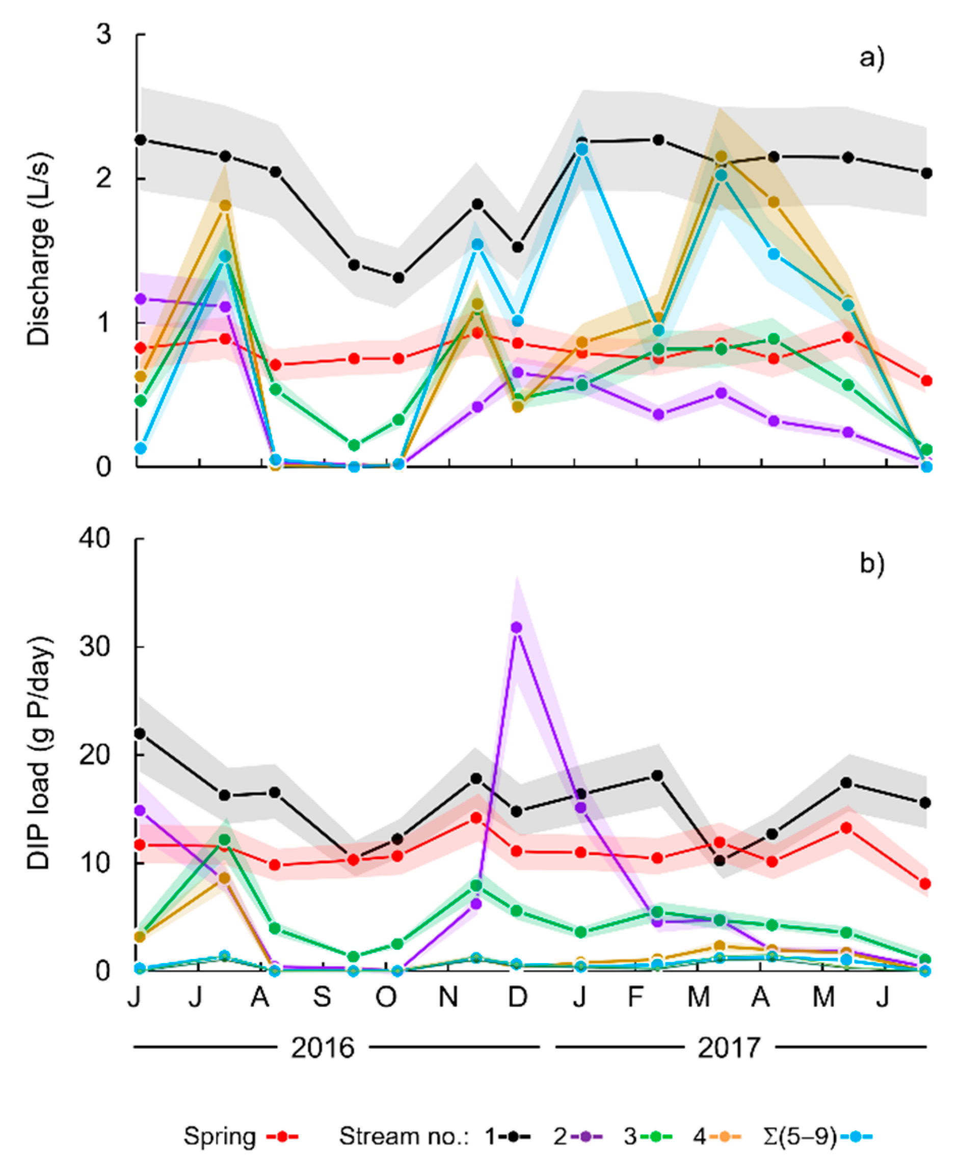
3.4. Stream and Spring Discharge and DIP Load to the Lake

Figure 6 shows the rates of stream and spring discharge (L/s) and the corresponding DIP load (g P/day) to the lake (note that streams 5–9 are summed). The depicted uncertainty bands (shaded areas) for the discharge in Figure 6a are based on the conducted discharge measurement uncertainty determination and represent ±1 standard deviation. The uncertainty bands for the DIP load in Figure 6b only reflect the discharge uncertainty as the analysis uncertainty for the DIP concentration is assumed relative small.

Throughout the year stream 1 accounted for the largest water inflow, with an annual mean discharge of 2 L/s (Figure 6a). The discharge in stream 1 started to decrease at the end of August and then increased again in October, likely caused by a gradual blockage and later cleaning of an under-road connecting tube upstream of the measurement point, which is typically carried out in the late autumn. In contrast, the spring showed a very stable discharge throughout the sampling period, though with an annual mean discharge of 0.8 L/s, which was less than half of the value for stream 1. Nevertheless, stream 1 and the spring were both important contributors of external DIP due to their high DIP concentrations (cf. Figure 5a), which corresponded to average DIP loads of 15.4 g P/day and 11.3 g P/day, respectively (Figure 6b).

In mid-June to mid-August 2016 and at the beginning of December 2016 to mid-February 2017, stream 2 also contributed with a substantial amount of DIP. The average load of DIP in these two periods were 11.6 g P/day and 23.5 g P/day, respectively. However, during the rest of the year, stream 2 had a low to non-existing DIP load, which can be attributed to low to non-existing discharge in stream 2 during these months (Figure 6a). Accordingly, stream 2 only had an annual mean DIP load of 7.5 mg P/L and thus stream 1 and the spring were the two main DIP contributors.

Streams 3 and 4 both had approximately the same annual mean discharge rate as the spring (stream 3: 0.7 L/s; stream 4: 0.9 L/s). However, as their DIP concentrations were low (cf. Figure 5a), their DIP loads were likewise significantly less than that of the spring (stream 3: 4.9 g P/day; stream 4: 1.8 g P/day).

Streams 5 to 9 contributed with the lowest DIP loads ranging from 0.0 to 0.3 g P/day as a result of low DIP concentrations and low discharge rates, all less than 0.5 L/s.

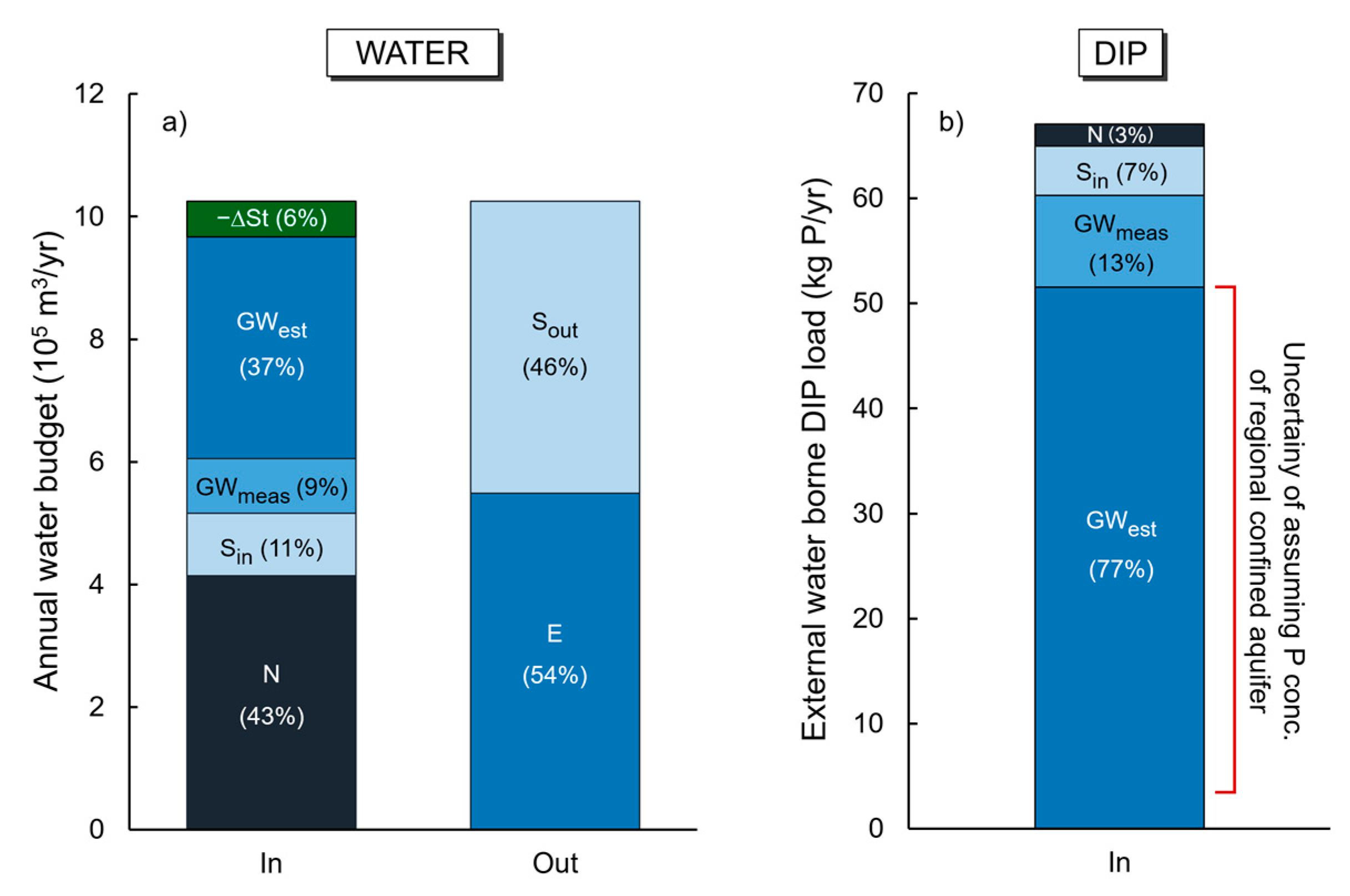
3.5. Annual Water Budget and DIP Load to Nørresø

The total water outflow from Nørresø was 10.2 × 10⁵ m³/year (Figure 7a), as calculated for the hydrological year 6 June 2016 to 21 June 2017. Taking into account a lake water volume of approximately 16 × 10⁸ m³, this corresponded to a lake hydraulic retention time of 1.6 years.

Precipitation and evaporation represented the major water input and output, respectively, to Nørresø, accounting for 43% and 54%.

The isotopic and hydrochemical composition of the groundwater, the spring, and water in the nine streams were used as tracers to differentiate streams discharging ‘deep’ groundwater derived from the regional confined aquifer from streams discharging ‘shallow’ groundwater, as derived from shallower circulation systems, or surface runoff. Based on this, the spring and only one of the streams (No. 1; located near the spring) was assumed to discharge deep groundwater from the regional confined aquifer to the lake (the derivation of this is presented in Section 4). Conditional on this differentiation, the deep groundwater discharge was partly measured (GW_meas) and accounted for 9% of the total water input. Shallow groundwater or surface runoff discharging from the remaining eight streams (Nos. 2–9) only accounted for 11% of the water input. Surface water output via the outlet accounted for 46% of the water loss.

By combining the water outputs from the lake and taking into account the decline in the water level during the investigated hydrological year (ΔSt), it is evident that the water output exceeded the detected total water input (cf. Equation 1). The missing water in the water budget is believed to have stemmed from undiscovered groundwater seepage areas at the bottom of the lake. This estimated groundwater (GW_est) input accounts of 37% the water input to the lake, so that the total groundwater input adds up to 46% (GW_meas + GW_est). Bearing in mind the continuous upwards hydraulic gradients to the lake (cf. Section 3.2), a negligible downwards groundwater recharge from the lake was assumed.

For the DIP budget an assumption has to be made regarding the DIP load carried by the estimated groundwater input. Assuming the estimated groundwater input came from the regional confined aquifer and carried an average DIP concentration as represented by the spring (4.6 µM), the estimated and measured groundwater input represented by far the largest share of the external water-borne DIP to the lake, contributing 77% and 13% of the DIP load, respectively (Figure 7b). Also, with this assumption, the annual water-borne external DIP load to Nørresø amounted to 67 kg P/year (Figure 7b). Stream discharge composed of surface runoff or shallow groundwater (i.e., streams 2–9) accounted for just 7% of the DIP load of which almost half of the DIP load is from stream 2 alone. Precipitation contributed with only ~3% of the annual water-borne DIP load to the lake, assuming that the precipitation DIP load equaled the atmospheric deposition of 1.3 mol TP/ha/year [47]. The uncertainty related to the assumption of the DIP concentration of the GW_est component will be discussed in Section 4.

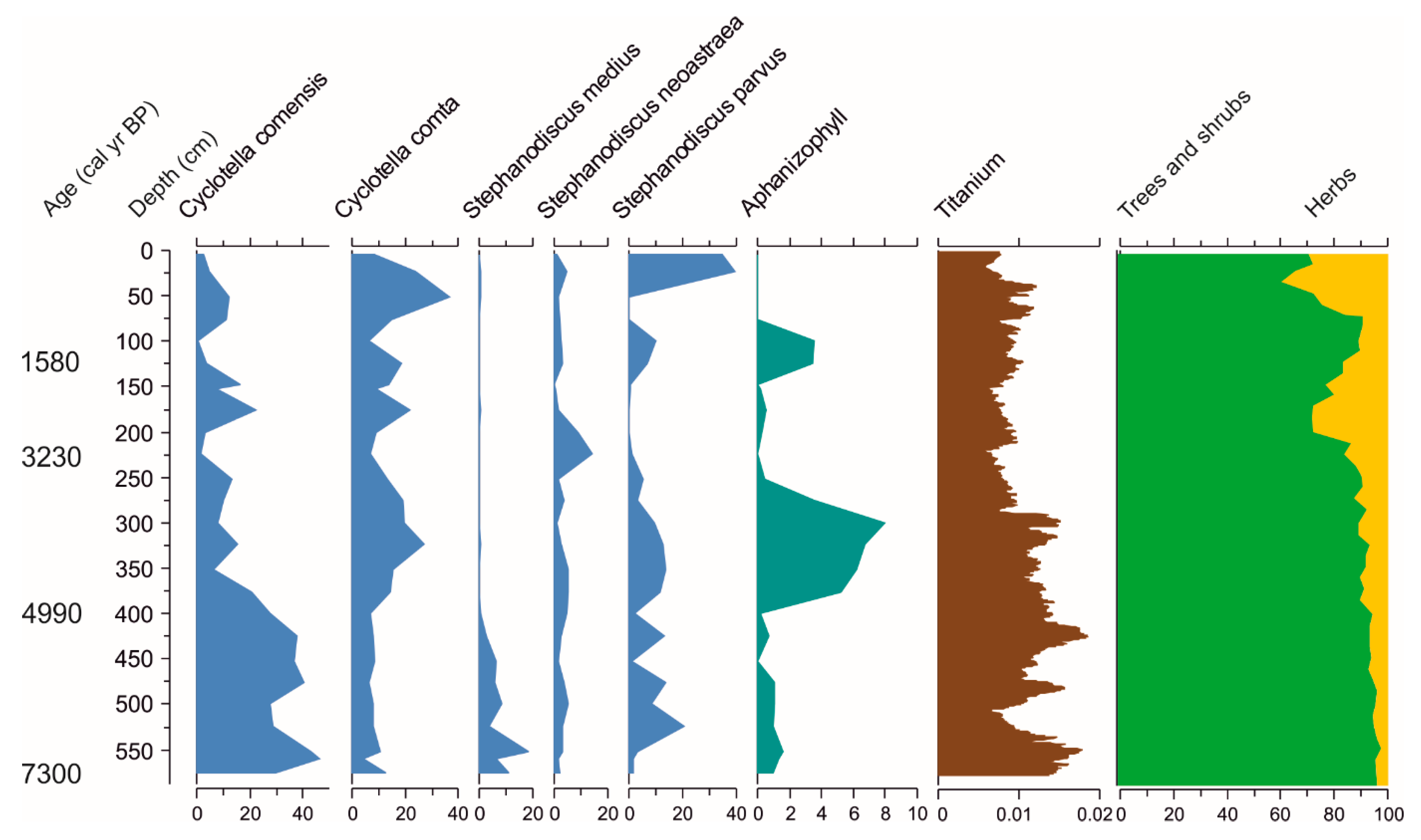
3.6. Paleolimnological Analyses

Figure 8 presents percentage abundances of dominant diatom species in the sediment stratigraphy, aphanizophyll, which is a pigment specific to filamentous cyanobacteria, normalized titanium data, and the percentage of tree/shrub and herb pollen indicative of land use changes in the catchment area of Nørresø. Dominant diatom species throughout the core include Cyclotella comensis, Cyclotella comta, Stephanodiscus medius, Stephanodiscus neoastraea, and Stephanodiscus parvus. The lower part of the core, from ca. 7500–5000 cal yr BP, is characterized by the highest abundances of Cyclotella comensis and Stephanodiscus medius, after which especially Cyclotella comta becomes more abundant. Stephanodiscus parvus, which is a common constituent of hypertrophic lakes, was relatively abundant throughout the core (ca. 10–20%), reaching ca. 40% in the most recent parts of the sediment stratigraphy. Aphanizophyll concentrations were ca. 0.5–1.5 nmol/g dry weight (DW) throughout most of the core, apart from two periods of elevated concentrations between ca. 5000 and 3300 cal yr BP and around 1500 cal yr BP. Tree and shrub pollen dominated throughout the sediment stratigraphy. Their percentage abundance was ≥90% until ca. 3000 cal yr BP, after which forest clearance (for pastures and fields) was evident as a decrease in tree/shrub pollen abundance and an increase in herb pollen during two distinctive periods. However, even here the total tree/shrub percentage did not decrease below ca. 60%, suggesting a mainly forested lake catchment throughout Holocene. This was supported by titanium (Ti), an unambiguous indicator of allochthonous inputs from the catchment, which showed low amounts and little variability unrelated to the forest clearance suggested by pollen data, and to the algal indicators of lake trophy.

4. Discussion

Present day DIP concentrations (2–20 µM) in the lake exceeded by far the threshold for the trophic class eutrophic (TP > 1 µM; [23]) and in some months even the threshold for the hypereutrophic class (TP > 3 µM; [23]). Hence, under the current condition the lake did not achieve “good ecological status”. In order to restore and improve eutrophic freshwater ecosystems it is necessary to identify and determine the relative P load of the different external sources of DIP to the lake [6,7,8,9].

Using geochemical attributes as a tracer [45,48], we discuss in the following subchapters which streams were mostly fed by water from the regional confined aquifer and which were mostly fed from other sources, such as groundwater with a shallower circulation system or surface runoff. Subsequently the main external sources of water-borne DIP was identified.

4.1. Identifying Deep Groundwater Discharge

The 14 drillings conducted near the lakeshore and the lithological logs from the three nearby water supply wells, together with the slow hydraulic response of the seven piezometers, indicated clayey till from within the upper 1–2 m below terrain to more than 35 m depth, which showed that the catchment area of Nørresø and the lake itself is located in a low permeable lithology.

The presence of the (artesian) spring on Lucieø demonstrated, however, that a confined aquifer must exist below the till bed, which was also evident from the lithological logs of the water supply wells.

In humid climate zones such as Denmark, it is generally considered that the δ²H and δ¹⁸O isotope composition in groundwater is a representative mixture of weighted average annual rainfall [49], and that the groundwater temperature corresponds closely to the average annual air temperature. Accordingly, both parameters were assumed constant in the regional confined aquifer throughout the year. The constant stable isotopic composition of the spring water matrix as well as its constant temperature of ~9 °C (Danish groundwater temperature is 8–9 °C; [44]) therefore substantiated that the spring discharged groundwater from the regional confined aquifer, rather than shallowly circulated groundwater or surface runoff, to the lake. This was further consistent with the identical isotopic composition of the spring and the confined aquifer (i.e., both below the isotopic group 1). Using the same line of reasoning of identical isotopic composition and constant temperature, water in stream 1 most likely also originated directly from the confined aquifer. Accordingly, stream 1 likely drain the meadow from a constant supply of confined aquifer groundwater, rather than from surface runoff or precipitation.

The assumption that the spring and stream 1 are fed by groundwater from the regional confined aquifer is further substantiated by the highly comparable chemical compositions (high concentrations of Fe²⁺ > 20 µM and low concentrations of O₂ < 0.004 mM) of the confined aquifer water matrices, with the spring and stream 1 water matrices. Concurrently, the elevated concentrations of DIP in the spring (mean 4.6 µM) and stream 1 (mean ~3 µM) were consistent with the high TP concentrations measured in the confined aquifer (mean ~5 µM).

Indications that the regional confined aquifer approached the terrain close to the area where the spring and stream 1 are located are found in the ERT data, acquired between the meadow and the east end of Nørresø (NE ERT). The ERT data profile (not shown) reflected a sloping layer of sand, connecting a deep-lying sand layer (i.e., the confined aquifer) and the terrain. This observation supported the suggestion that the spring on Lucieø and stream 1 tap the regional aquifer.

According to the annual water budget, groundwater discharge to the lake accounted for 46% of the total water input. One quarter of this groundwater input was directly measured as the summed discharge of stream 1 and the spring, while three quarters were deducted from the water budget.

From a stratigraphic viewpoint, it seemed highly unlikely that a sand seam through which the groundwater was discharging occurred only at one location. Thus, it is likely that that the confined aquifer also approached the surface at other locations under the lake. Accordingly, this would explain the relatively large estimated groundwater component. The significant elevation of the spring, relative to the lake surface (>+1 m), indicated further that the estimated groundwater input must enter the lake via small-scale discrete discharge zones in the lakebed, rather than through diffuse inflow over one or more laterally extensive connection(s) with the sandy aquifer, which would equalize the hydraulic pressure of the aquifer (spring) and the lake much more.

4.2. Identifying Discharge of Shallow Groundwater or Surface Runoff

The above water budget considerations showed that isotopic group 1 (i.e., the spring, stream 1, and the regional confined aquifer) represented groundwater with more or less constant δ-values. The isotopic composition of group 1 was significantly different from the δ-values in group 2 (i.e., streams 3, 5, 6, 8, and 9) as well as in group 3 (i.e., streams 2, 4, and 7) (Figure 3). This strongly suggested that the discharging water from the streams in these two groups had different origins and different flow paths. The temporal variation in the isotopic δ-values was more pronounced in isotopic group 3 (for stream 2 in particular), as compared to group 2, which again was more variable than group 1 (i.e., groundwater from the regional confined aquifer).

Sub-annual fluctuations in water isotopic composition, when they occur close to the LMWL, most likely reflected seasonal isotopic variations in the precipitation feeding the streams and, consequently, sub-annual residence times for at least a part of the stream discharge. This short-term variability may be associated to surface runoff or groundwater in shallow circulation systems, or a mixture of these.

The ephemeral (streams 2 and 4–9) or variable-discharge (stream 3) characteristics of these streams (i.e., 2–9) further supported a larger fraction of water with sub-annual residence times in contrast to continual base flow dominance. In addition, streams 2–9 all showed large temperature fluctuations and oxidized conditions (Fe²⁺ < 1.4 µM and close-to-saturation O₂) which did not reflect the anoxic groundwater. However, these parameter characteristics may have resulted from exposure to ambient conditions along longer stream stretches rather than from the source of the water. Nevertheless, streams 2–9 are likely to primarily represent discharging shallow groundwater or surface runoff, rather than water from the deep regional confined aquifer.

In contrast to the groundwater from the confined aquifer, the DIP concentrations were relatively low in the majority of the streams discharging shallow groundwater or surface runoff, with the exception of stream 2. Stream 2, as mentioned earlier, seasonally discharged water from a small lake, Hjertesø, which explains its elevated DIP concentrations and its more extreme temporal δ-values variation caused by evaporation from this lake’s water surface.

4.3. Water Budget and External Water-Borne DIP Load to Nørresø

According to the water budget, precipitation accounted for 43% of the total annual water input to the lake, whereas it only contributed ~3% of the annual water-borne DIP load to the lake. This demonstrated that there was no direct relationship between water input and P loading between different sources. Shallow groundwater water or surface runoff (i.e., discharge of streams 2–9) accounted for 11% of the water input and just 7% of annual water-borne DIP load, of which stream 2 (feeding water from Hjertesø) accounted for almost half. The measured groundwater input (sum of the spring and stream 1, GW_meas) accounted for just 9% of the annual water input to the lake, but was still the second largest DIP contributor, accounting for 13% of the total water-borne DIP load to lake.

When GW_meas was combined with the estimated groundwater (GW_est) component and if the latter was assumed to carry an average DIP concentration representative for the regional confined aquifer (the spring’s 4.6 µM), then groundwater discharge contributed to half of the total annual water input to the lake and with 90% of the annual water-borne external DIP load to the lake. However, this assumption (i.e., of the (unmeasured) DIP concentration of GW_est) introduced uncertainty in the DIP budget. If the estimated groundwater input was assumed to carry a much smaller DIP concentration, for example the 0.3 µM DIP concentration of streams 5, 7, and 9 (Section 3.3.3), then the DIP load related to GW_est would have been reduced from 52 kg P/year to just 3.4 kg P/year. This offset is indicated as uncertainty to the right of the DIP budget column in Figure 7b. A low DIP concentration could reflect that the estimated groundwater input was actually shallow (not deep) groundwater or even unmeasured surface runoff. While the uncertainty range allows a reduction in the total DIP load by almost 50 kg P/year, to just 19 kg P/year, still the actually measured groundwater-borne DIP load of ~9 kg P/year would account for nearly half of the total DIP load, i.e., 9 out of 19 kg P/year. Furthermore, neglecting any unmeasured surface runoff so that GW_est is assumed to be some source of groundwater with at least a 0.3 µM DIP concentration, then groundwater-borne DIP will amount to at least 64% of the annual DIP load to the lake.

This serves as a clear example that groundwater-borne DIP can be a significant source of P entering freshwater ecosystems. The estimated groundwater P contribution was at a significantly higher level than previously assumed for this lake. Fyn’s County [27] estimated that groundwater only accounted for 16% of the annual water-borne TP load to Nørresø. Although that study dealt with TP and not DIP, the different results underline the importance of a thorough study of water and P budget components for understanding P budgets.

One of the main challenges in identifying hydrological budgets for a lake lies in quantifying the groundwater fluxes [16]. As in the present study, this flux has often been determined as the residual of the water budget [34]. In cases where both groundwater discharge and groundwater recharge are unknown only the net groundwater component (i.e., the difference of discharge and recharge) is identified. Considering different P concentrations of groundwater and lake water, this results in erroneous P budgets based on the “residual” approach [16]. The present approach is, thus, only applicable for estimations of P loadings if groundwater-lake gradients consistently show groundwater discharge to the lake (like in the present study).

Bearing in mind that the estimated groundwater component in the present study is quantified as the residual in the water budget, all measurement uncertainties are consequently accumulated in the estimated groundwater component. The studied hydrological year was unusual in the sense that evaporation exceeded precipitation; usually for Danish catchments the opposite is the case. Nevertheless, the evaporation component was not measured directly and if its estimation in the present year led to an overestimation, then this would result also in an overestimation of the groundwater DIP loading.

In contrast, the measured water output via the outlet represented a minimum water discharge. Installation of the flume introduced resistance to the stream flow, which required equilibration to a new higher stationary water level in the stream reach upstream the flume. The conditions in all streams (1–9) allowed such equilibration within a few minutes. In the outlet, however, equilibration would require the level of the whole lake to increase to the new stationary water level which, of course, was practically infeasible. Therefore, the flume readings (which reflected the upstream water level) must have been too low, resulting in too low discharge determinations. The underestimation of the outlet discharge implies that the water balance residual, and thereby the estimated groundwater input (GW_est) and associated DIP load, were also underestimated.

Accordingly, the interpretation of the water budget and associated DIP loadings is somewhat uncertain. Nevertheless, a large certainty persists regarding the amounts and relative importance of the actual measured groundwater-borne DIP load vs. the DIP load fed by streams 2–9. Therefore, the groundwater-borne DIP load to the lake constituted minimum ca. half, and likely at least 64% of the total water-borne DIP load. Uncertainties are mainly related to the total DIP load (amount) and to which percentage in between 64% and 90% of the total DIP load is correct for the groundwater-borne DIP contribution.

The findings in the present study underline the benefit of conducting a combined investigation of both water chemistry, isotopic tracers, temperature, and water volume fluxes, with a dense temporal resolution. Nørresø has many small inlets and the frequent measurements of fluxes and geochemistry of these streams has revealed that the lake is dominated by groundwater-borne DIP input to the lake, although groundwater input is of only secondary importance in the lake’s water budget.

4.4. Origin of the Dissolved Inorganic Phosphorus

The sources of DIP in the water discharging in streams 2–9 should be found at or near the surface, rather than in the regional confined aquifer. The DIP concentration of stream 2 is obviously controlled by internal P cycling in the small lake (Hjertesø) drained by this stream as concluded above. Stream 3 received water from drainage pipes connected to a large agricultural field located west of Nørresø (Figure 2) and contained elevated concentrations of NO₃⁻ (average 0.63 mM; Figure 5d). Thus, the DIP in stream 3, which is the third most important stream in terms of annual DIP loading to the lake, properly originated from fertilizers.

NO₃⁻ was also detected in streams 4 and 5 with average concentrations of 0.2 and 0.15 mM, respectively. Stream 4 is located close to a conifer plantation and stream 5 is close to an agricultural field (Figure 2). The (small; Figure 6) DIP loading associated with streams 4 and 5 may accordingly also be influenced by agriculture.

The observed elevated DIP concentrations in the spring and stream 1 is attributed to the discharge of P-rich groundwater from the regional confined aquifer. The probability that anthropogenic-induced P-enriched water has percolated down through the thick confining clay layer and subsequently reached the underling sand-aquifer resulting in the elevated groundwater TP concentrations is highly unlikely [35,50]. The mobile P in the confined aquifer, hence, more likely resulted from mobilization of geogenic phosphorus within the aquifer.

Numerous studies show a correlation between the mobilization of DIP and sediment redox conditions [11,12,22]. Particularly, the reduction of Fe-oxides [11,15], and in some cases also manganese oxides [13], will lead to a mobilization of DIP. The high concentrations of Fe²⁺ and the reducing conditions in the regional confined aquifer are thus consistent with the theory of natural release of DIP from reductive dissolution of Fe-oxides.

A shift in the redox condition might explain why the DIP concentration in stream 1 was lower than the one detected in the spring, even though the water is evaluated to have the same origin. The discharging water in stream 1 had a longer flow path through oxidizing conditions from the groundwater seepage area (the meadow, Figure 1) to the lake, giving time for Fe-oxide precipitation and thus depletion of DIP via co-precipitation and adsorption.

Spontaneous precipitation of Fe-oxides will most likely also occur when anoxic, ferrous P-rich groundwater enters the oxic lake water column. This process would affect lake DIP concentrations through adsorption or co-precipitation. However, the Fe-oxides with adsorbed P will be accumulated on the lakebed and become a part of the internal mobile P pool, which potentially is released to the water column during summer anoxia at the lakebed. The impact of internally released P and the role of accumulated Fe-oxides with adsorbed P in Nørresø were investigated and discussed by Nisbeth et al. [31]. Their results strongly suggests that groundwater-transported geogenic P was the original source of the now internally cycled P and that this mechanism was mainly driven by the reductive dissolution of Fe-oxides.

The elevated P concentration in the groundwater could also be attributed to degradation of buried organic matter. However, the observed mol:mol ratios of dissolved NH₄⁺-to-DIP in groundwater of the confined aquifer (~4; [32]) were somewhat lower than the N:P ratio of organic matter (~16), indicating that organic matter-bound P is not the main component of the P in the groundwater of the confined aquifer.

4.5. Paleolimnological Indicators for P Sources to the Lake

To further substantiate the hypothesis that groundwater-transported geogenic P has been the dominant external source of P entering the lake, we applied diatom, pigment, XRF, and pollen analyses on a ca. 6-m-long sediment core section collected from the central part of the lake (Figure 2).

Diatom analyses of core samples, dating from before the introduction of agriculture (i.e., older than 6000 cal yr BP), showed dominance of Cyclotella comensis, C. comta, and Stephanodiscus medius, with smaller contributions (up to ca. 10% of the assemblage) by S. neoastraea and S. parvus, indicating that even in the pristine state the lake was already meso-eutrophic [51]. This strongly suggested that natural nutrient enrichment of Nørresø has occurred. The diatom assemblages of the whole sediment record suggested, in addition, that the lake water was never P-poor, which is consistent with current conditions (Figure 8).

Carotenoid pigments from filamentous bloom-forming cyanobacteria (aphanizophyll and/or myxoxanthophyll) are almost consistently present in the sediment record of Nørresø for the last 7500 years (Figure 2). Such cyanobacteria are commonly associated with low N:P ratios because of their ability to fix atmospheric nitrogen. Their persistence in Nørresø is probably connected with the high P supply. Naturally high abundances of cyanobacteria are observed in other lakes on glacial moraine landscapes where groundwater supply dominates [52]. Debate still exists, however, about the relative roles of groundwater supply and internal recycling of P in such lakes with very low flushing rates [53]. Nevertheless, the strong indication of filamentous cyanobacteria persistence throughout the last 7500 years of Nørresø’s history supports the assumption of groundwater being an important source of DIP to the lake.

For some lakes particulate P accounts for a substantial proportion of the total external P loading [54], especially during high rainfall were soil erosion is accelerated. The monthly measurements of discharge and water chemical parameters may not have captured high flow events. Hence, particulate P could constitute an impotent external P source entering Nørresø. Pollen analysis indicates, however, that the lake catchment was predominantly forested throughout its Holocene history (Figure 8). This is consistent with historical and present day conditions, where 88% of the topographical catchment is covered by forest and 12% by agriculture [27,28]. A dominantly forested catchment makes particulate P transport to the lake by soil erosion less likely. Furthermore, low and relatively invariable concentrations of the soil erosion indicator Ti [55] (Figure 8) indicates that little erosion from the catchment occurred throughout the history of Nørresø. Also, the variability of Ti is unrelated to changes in the algal trophic indicators. This strongly suggest that other main transporters of P, such as DIP with groundwater, are more important for the trophic state of Nørresø.

A possible additional source of P could be leaves and other organic detritus from the catchment causing gradual and progressing eutrophication through the lake’s ontogeny. There has, however, never been documented long-term natural eutrophication due to catchment organic detritus. In contrast, ample documentation of the opposite process (i.e., natural long-term oligotrophication) occurring in ecosystems without additional anthropogenic or geogenic influence such as during interglacials (terrestrial [56], lacustrine [57]) as well as during the Holocene in lakes in subtropical [58], temperate [59], and boreal [60] zones is published. Accordingly, it is highly unlikely that the natural eutrophication of Nørresø through the Holocene was driven by P input from catchment organic detritus. Combining the paleolimnological results with the modern measurements strongly suggests groundwater to be a highly important external source of DIP in the case of Nørresø and potentially in the case of other surface water bodies. The first important implication of this conclusion is that very significant releases of geogenic DIP to groundwater may occur naturally within aquifers or near the surface in the recharge area.

In the present study area, the elevated DIP concentrations in the deep confined aquifer signify that the P release occurred long before the groundwater reached the near-lake area (water supply wells with elevated groundwater TP concentrations are more the 3 km away from the spring). The second implication therefore is that phosphorus can be transported with groundwater over at least distances of a couple of km.

In the case of Nørresø, some deforestations during the periods 3000–2000 ca yr BP and again 800–0 cal yr BP seems to have occurred, caused by domestic grazing and arable farming. These anthropogenic disturbances could have caused some cultural eutrophication, as, for example, seen in the last ca. 800 years as peak abundances of Cyclotella comta and Stephanodiscus parvus. However, the dominance of meso-eutrophic diatom assemblages together with the occurrence of filamentous cyanobacteria long before increased anthropogenic pressure on the catchment area of Nørresø are consistent with the current situation where just a fraction (~10%) of the external DIP load is believed to originate from fertilizers and nutrient enrichment from non-cultural sources is of major importance for the trophic status of the lake.

5. Conclusions

This cross-disciplinary study found the presence of a regional artesian aquifer with high concentrations of geogenic P, which ultimately end up in the lake via groundwater discharge. This was deduced from combining the water budget-derived groundwater contribution with observations of lithology, hydraulic heads, and temperature, isotopic, and hydrochemical tracers. In addition, results from paleolimnological studies indicated that the lake was never P-poor due to dissolved P inputs, even before agricultural disturbances. In combination, these results are of relevance for understanding global terrestrial P cycling in that they provide evidence for:

• Phosphorus transport with groundwater over long (km) distances;
• Natural significant releases of geogenic phosphorus to groundwater;
• Groundwater-borne dissolved inorganic phosphorus can potentially be the main contributor of P to surface freshwater ecosystems. In the studied lake, Nørresø, groundwater inputs accounted for 90% of the total annual external DIP load, even though groundwater constituted only one third of water input to the lake.

Finally, the study demonstrates the clear benefits in the field of water resources research of combining lithological observations with dense temporal observations of multiple tracers, hydraulic heads and water volume fluxes, and paleolimnological observations.

References

1. Søndergaard, M.; Jeppesen, E. Anthropogenic impacts on lake and stream ecosystems, and approaches to restoration. J. Appl. Ecol. 2007, 44, 1089–1094. [Google Scholar] [CrossRef]
2. UNEP. Environment for the Future We Want; Progress Press Ltd: Valletta, Malta, 2012; ISBN 9789280731774. [Google Scholar]
3. EEA. Assessment of Global Megatrends—An Update. Global Megatrend 1: Diverging Global Population Trends; European Environment Agency: Copenhagen, Denmark, 2014.
4. Hecky, R.E.; Kilham, P. Nutrient limitation of phytoplankton in freshwater and marine environments: A review of recent evidence on the effects of enrichment1. Limnol. Oceanogr. 1988, 33, 796–822. [Google Scholar] [CrossRef] [Green Version]
5. Blake, R.E.; O’Neil, J.R.; Surkov, A.V. Biogeochemical cycling of phosphorus: Insights from oxygen isotope effects of phosphoenzymes. Am. J. Sci. 2005, 305, 596–620. [Google Scholar] [CrossRef]
6. Vanek, V. The interactions between lake and groundwater and their ecological significance. Stygologia 1987, 3, 1–23. [Google Scholar]
7. Kilroy, G.; Coxon, C. Temporal variability of phosphorus fractions in Irish karst springs. Environ. Geol. 2005, 47, 421–430. [Google Scholar] [CrossRef]
8. Holman, I.P.; Whelan, M.J.; Howden, N.J.K.; Bellamy, P.H.; Willby, N.J.; Rivas-Casado, M.; McConvey, P. Phosphorus in groundwater—An overlooked contributor to eutrophication? Hydrol. Process. 2008, 22, 5121–5127. [Google Scholar] [CrossRef]
9. Holman, I.P.; Howden, N.J.K.; Bellamy, P.; Willby, N.; Whelan, M.J.; Rivas-Casado, M. An assessment of the risk to surface water ecosystems of groundwater P in the UK and Ireland. Sci. Total Environ. 2009, 408, 1847–1857. [Google Scholar] [CrossRef] [PubMed]
10. Heiberg, L.; Pedersen, T.V.; Jensen, H.S.; Kjaergaard, C.; Hansen, H.C.B. A comparative study of phosphate sorption in lowland soils under oxic and anoxic conditions. J. Environ. Qual. 2010, 39, 734–743. [Google Scholar] [CrossRef] [PubMed]
11. Kjaergaard, C.; Heiberg, L.; Jensen, H.S.; Hansen, H.C.B. Phosphorus mobilization in rewetted peat and sand at variable flow rate and redox regimes. Geoderma 2012, 173–174, 311–321. [Google Scholar] [CrossRef]
12. Prem, M.; Hansen, H.C.B.; Wenzel, W.; Heiberg, L.; Sørensen, H.; Borggaard, O.K. High Spatial and Fast Changes of Iron Redox State and Phosphorus Solubility in a Seasonally Flooded Temperate Wetland Soil. Wetlands 2015, 35, 237–246. [Google Scholar] [CrossRef]
13. Walter, D.A.; Rea, B.A.; Sollenwerk, K.G.; Savoie, J. Geochemical and Hydrologic Controls on Phosphorus Transport in a Sewage Contaminated Sand and Gravel Aquifer Near Ashumet Pond, Cape Cod, Massachusetts; Technical Report; United States Geological Survey: Reston, VA, USA, 1996.
14. Burkart, M.R.; Simpkins, W.W.; Morrow, A.J.; Gannon, J.M. Occurrence of total dissolved phosphorus in unconsolidated aquifers and aquitards in Iowa. J. Am. Water Resour. Assoc. 2004, 40, 827–834. [Google Scholar] [CrossRef]
15. Griffioen, J. Extent of immobilisation of phosphate during aeration of nutrient-rich, anoxic groundwater. J. Hydrol. 2006, 320, 359–369. [Google Scholar] [CrossRef]
16. Lewandowski, J.; Meinikmann, K.; Nützmann, G.; Rosenberry, D.O. Groundwater—The disregarded component in lake water and nutrient budgets. Part 2: Effects of groundwater on nutrients. Hydrol. Process. 2015, 29, 2922–2955. [Google Scholar] [CrossRef]
17. Meinikmann, K.; Lewandowski, J.; Hupfer, M. Phosphorus in groundwater discharge—A potential source for lake eutrophication. J. Hydrol. 2015, 524, 214–226. [Google Scholar] [CrossRef]
18. Kidmose, J.; Nilsson, B.; Engesgaard, P.; Frandsen, M.; Karan, S.; Landkildehus, F.; Søndergaard, M.; Jeppesen, E. Focused groundwater discharge of phosphorus to a eutrophic seepage lake (Lake Væng, Denmark): Implications for lake ecological state and restoration. Hydrogeol. J. 2013, 21, 1787–1802. [Google Scholar] [CrossRef]
19. Kazmierczak, J.; Müller, S.; Nilsson, B.; Postma, D.; Czekaj, J.; Sebok1, E.; Jessen, S.; Karan, S.; Stenvig Jensen, C.; Edelvang, K.; et al. Groundwater flow and heterogeneous discharge into a seepage lake: Combined use of physical methods and hydrochemical tracers. Water Resour. Res. 2016, 52, 9109–9130. [Google Scholar]
20. Shaw, R.D.; Shaw, J.F.H.; Fricker, H.; Prepas, E.E. An integrated approach to quantify groundwater transport of phosphorus to Narrow Lake, Alberta. Limnol. Oceanogr. 1990, 35, 870–886. [Google Scholar] [CrossRef]
21. Kenoyer, G.; Anderson, M.P. Groundwater’s dynamic role in regulating acidity and chemistry in a precipitatuon-dominated lake. J. Hydrol. 1989, 109, 287–306. [Google Scholar] [CrossRef]
22. Szilas, C.P.; Borggaard, O.K.; Hansen, H.C.B. Potential iron and phosphate mobilization during flooding of soil material. Water. Air. Soil Pollut. 1998, 106, 97–109. [Google Scholar] [CrossRef]
23. Wetzel, R.G. The Phosphorus Cycle. In Limnology: Lake and River Ecosystems; Academic Press: San Diego, CA, USA, 2001; pp. 242–250. ISBN 9780127447605. [Google Scholar]
24. Anderson, N.J. Naturally eutrophic lakes: Reality, myth or myopia? Trends Ecol. Evol. 1995, 10, 137–138. [Google Scholar]
25. Søndergaard, M.; Jensen, J.P.; Jeppesen, E. Internal phosphorus loading in shallow Danish lakes. Hydrobiologia 1999, 408–409, 145–152. [Google Scholar] [CrossRef]
26. House, W.A. Geochemical cycling of phosphorous in rivers. Appl. Geochem. 2003, 18, 739–748. [Google Scholar] [CrossRef]
27. Fyn’s County. Nørresø 1989–1993, Lake Monitoring in Fyn’s County; Technical Report No. 1; Fyn’s County: Odense, Denmark, May 1994; 70p. [Google Scholar]
28. Odgaard, B.; Møller, P.F.; Wolin, J.A.; Rasmussen, P.; Anderson, N.J. Brahetrolleborg Nørresø. Palæolimnologisk Undersøgelse og Oplandsanalyse; Company Report (48); Denmark’s Geological Surveys: Copenhagen, Denmark, 1995; pp. 1–56. [Google Scholar]
29. Høy, T. Danmarks Søer—Søerne i Fyns Amt; Strandbergs Forlag: Charlottenlund, Denmark, 2000. [Google Scholar]
30. Moorleghem, V.C.; De Schutter, N.; Smolders, E.; Merckx, R. The bioavailability of colloidal and dissolved organic phosphorus to the alga Pseudokirchneriella subcapitata in relation to analytical phosphorus measurements. Hydrobiologia 2013, 709, 41–53. [Google Scholar] [CrossRef]
31. Nisbeth, C.S.; Jessen, S.; Bennike, O.; Kidmose, J.; Reitzel, K. Role of Groundwater-Borne Geogenic Phosphorus for the Internal P Release in Shallow Lakes. Water 2019, 11, 1783. [Google Scholar] [CrossRef]
32. Geological Survey of Denmark and Greenland (GEUS). Danish National Borehole Achieve (Jupiter). 2018. Available online: www.geus.dk (accessed on 21 September 2018).
33. Jørgensen, F.; Sandersen, P.B.E.; Auken, E. Imaging buried Quaternary valleys using the transient electromagnetic method. J. Appl. Geophys. 2003, 53, 199–213. [Google Scholar] [CrossRef]
34. Rosenberry, D.O.; LaBaugh, J.W. Field Techniques for Estimating Water Fluxes Between Surface Water and Ground Water Techniques and Methods; United States Geological Survey: Reston, VA, USA, 2008.
35. Fitts, C.R. Groundwater Science, 2nd ed.; Academic Press: Waltham, MA, USA, 2002; ISBN 9780123847058. [Google Scholar]
36. Det Nationale Overvågningsprogram for Vandmiljø og Natur (NOVANA). Available online: http://novana.dmi.dk/ (accessed on 3 April 2018).
37. Skogerboe, G.V.; Bennett, R.S.; Walker, W.R. Selection and Installation of Cutthroat Flumes for Measuring Irrigation and Drainage Water; Technical Bulletin 120; Colorado State University: Denver, CO, USA, December 1973. [Google Scholar]
38. Skogerboe, G.V.; Bennett, R.S.; Walker, W.R. Generalized Discharge Relations for Cutthroat Flumes. J. Irrig. Drain. Divis. 1972, 98, 569–583. [Google Scholar]
39. Stookey, L.L. Ferrozine—A New Spectrophotometric Reagent for Iron. Anal. Chem. 1970, 42, 779–781. [Google Scholar] [CrossRef]
40. Murphy, J.; Riley, J.P. A modified single solution method for the determination of phosphate in natural waters. Anal. Chim. Acta 1986, 27, 31–36. [Google Scholar] [CrossRef]
41. Reimer, P.J.; Bard, E.; Bayliss, A.; Beck, J.W.; Blackwell, P.G.; Ramsey, C.B.; Buck, C.E.; Cheng, H.; Edwards, R.L.; Friedrich, M.; et al. IntCal13 and Marine13 Radiocarbon Age Calibration Curves 0–50,000 Years cal BP. Radiocarbon 2013, 55, 1869–1887. [Google Scholar] [CrossRef]
42. Battarbee, R.W.; Jones, V.J.; Flower, R.J.; Cameron, N.G.; Bennion, H.; Carvalho, L.; Juggins, S. Diatoms. In Tracking Environmental Change Using Lake Sediments. Terrestrial, Algal, and Siliceous Indicators; Smol, J.P., Birks, H.J.P., Last, W.M., Eds.; Kluwer Academic Publishers: Dordrecht, The Netherlands, 2001; Volume 3, pp. 155–202. ISBN 9780306476686. [Google Scholar]
43. Faegri, K.; Iversen, J. Textbook of Pollen Analysis, 3rd ed.; Munksgaard: Copenhagen, Denmark, 1975. [Google Scholar]
44. Müller, S.; Stumpp, C.; Sørensen, J.H.; Jessen, S. Spatiotemporal variation of stable isotopic composition in precipitation: Post-condensational effects in a humid area. Hydrol. Process. 2017, 31, 3146–3159. [Google Scholar] [CrossRef]
45. Cirkel, D.G.; Van Beek, C.G.E.M.; Witte, J.P.M.; Van der Zee, S.E.A.T.M. Sulphate reduction and calcite precipitation in relation to internal eutrophication of groundwater fed alkaline fens. Biogeochemistry 2014, 117, 375–393. [Google Scholar] [CrossRef]
46. O’Connell, D.W.; Mark Jensen, M.; Jakobsen, R.; Thamdrup, B.; Joest Andersen, T.; Kovacs, A.; Bruun Hansen, H.C. Vivianite formation and its role in phosphorus retention in Lake Ørn, Denmark. Chem. Geol. 2015, 409, 42–53. [Google Scholar] [CrossRef]
47. Ellermann, T.; Bossi, R.; Christensen, J.; Løfstrøm, P.; Monies, C.; Grundahl, L.; Geels, C. Atmosfærisk Deposition 2014; Technical Report 163; Department of Environmental Sciences (DCE): Aarhus, Denmark, 2015. [Google Scholar]
48. Appelo, C.A.J.; Postma, D. Geochemistry, Groundwater and Pollution, 2nd ed.; Balkema: Rotterdam, The Netherlands, 2005; ISBN 9781439833544. [Google Scholar]
49. Clark, I.D.; Fritz, P. Environmental Isotopes in Hydrogeology; Lewis: Boca Raton, FL, USA; New York, NY, USA, 1997; ISBN 1566702496. [Google Scholar]
50. Cucarella, V.; Renman, G. Phosphorus sorption capacity of filter materials used for on-site wastewater treatment determined in batch experiments—A comparative study. J. Environ. Qual. 2009, 38, 381–392. [Google Scholar] [CrossRef] [PubMed]
51. Battarbee, R.W.; Juggins, S.; Gasse, F.; Anderson, N.J.; Bennion, H.; Cameron, N.G.; Ryves, D.B.; Pailles, C.; Chalie, F.; Telford, R. European Diatom Database (EDDI): An Information System for Palaeoenvironmental Reconstruction; Environmental Change Research Centre (ECRC) Report 81; University College London: London, UK, 2001. [Google Scholar]
52. McGowan, S.; Britton, G.; Haworth, E.; Moss, B. Ancient blue-green blooms. Limnol. Oceanogr. 1999, 44, 436–439. [Google Scholar] [CrossRef] [Green Version]
53. Kilinc, S.; Moss, B. Whitemere, a lake that defies some conventions about nutrients. Freshw. Biol. 2002, 47, 207–218. [Google Scholar] [CrossRef]
54. Carpenter, S.R.; Booth, E.G.; Kucharik, C.J.; Lathrop, R.C. Extreme daily loads: Role in annual phosphorus input to a north temperate lake. Aquat. Sci. 2014, 77, 71–79. [Google Scholar] [CrossRef]
55. Cohen, A.S. Paleolimnology: The History and Evolution of Lake Systems; Oxford University Press: New york, NY, USA, 2003. [Google Scholar]
56. Kuneš, P.; Odgaard, B.V.; Gaillard, M.J. Soil phosphorus as a control of productivity and openness in temperate interglacial forest ecosystems. J. Biogeogr. 2011, 38, 2150–2164. [Google Scholar] [CrossRef]
57. Kupryjanowicz, M.; Fiłoc, M.; Czerniawska, D. Occurrence of slender naiad (Najas flexilis (Willd.) Rostk. & W. L. E. Schmidt) during the Eemian Interglacial—An example of a palaeolake from the Hieronimowo site, NE Poland. Quat. Int. 2018, 467, 117–130. [Google Scholar]
58. Kenney, W.F.; Brenner, M.; Curtis, J.H.; Arnold, T.E.; Schelske, C.L. A holocene sediment record of phosphorus accumulation in shallow Lake Harris, Florida (USA) offers new perspectives on recent cultural eutrophication. PLoS ONE 2016, 11, e0147331. [Google Scholar] [CrossRef]
59. Odgaard, B.V. The Holocene vegetation history in northern West Jutland, Denmark. Opera Bot. 1994, 123, 1–171. [Google Scholar]
60. Norton, S.A.; Perry, R.H.; Saros, J.E.; Jacobson, G.L.; Fernandez, I.J.; Kopáček, J.; Wilson, T.A.; SanClements, M.D. The controls on phosphorus availability in a Boreal lake ecosystem since deglaciation. J. Paleolimnol. 2011, 46, 107–122. [Google Scholar] [CrossRef]
Figure 1. (a) Location of the Lake Nørresø in the southern part of Fyn, Denmark. (b) Overview of the numbering of streams, and the locations of stream sampling points and the outlet. The locations of the small island, Lucieø, hosting a spring and the small lake, Hjertesø, are also indicated. The dashed white lines indicate lake bathymetry (in meters; [29]). (c) The relative hydraulic head in seven piezometric wells placed at ~3 m depth. (d) Photo of the spring on the island Lucieø (black arrows indicate flow direction). Iron-oxides stain the bed of the 4-m-long stream which connects the spring to the lake.
Water 11 02213 g001
Figure 2. Overview of Nørresø and the surrounding area, and locations of piezometers, electrical resistivity tomography (ERT) profiles and the lakebed sediment core site. Lithological logs from the drillings (simplified to combine the shallow peat and the underlying clay till) and water supply wells are also included.
Water 11 02213 g002
Figure 3. δ18O and δ2H values for (a) all streams, the spring, the water supply wells and the lake. Panels (b,c) are subsets of panel (a); note the different range of the y- and x-axes. Group 1 and 2 in (b) represent clustered isotope data, while group 3 in (c) represents fluctuating isotope data. Local meteoric water line (LMWL) is from [44].
Water 11 02213 g003
Figure 4. Concentrations of Ca2+ and alkalinity of the streams, the spring, and the lake (Nørresø). The group number refers to the same stream grouping as presented for the isotope data (Figure 3). Lines indicate molar calcium:alkalinity ratios corresponding to calcite dissolution by carbonic acid (1:2) and strong acids (1:1).
Water 11 02213 g004
Figure 5. Boxplot showing concentrations of dissolved inorganic orthophosphate (DIP) (a), Fe2+ (b), O2 (c), and NO3 (d) and temperature (e) in the streams, the spring, Lake Nørresø, and in the regional confined aquifer. Note that along the x-axis the data for the different streams, the spring, and confined aquifer are grouped with respect to their isotopic grouping (cf. Figure 3). Lower and upper whisker indicates the minimum and maximum values, respectively, excluding statistical outliers. Median and mean value is depicted in each box by a straight horizontal line and a cross, respectively.
Water 11 02213 g005
Figure 6. (a) Discharge rates and (b) DIP load to Lake Nørresø from the spring (red) and streams 1 (black), 2 (purple), 3 (green), and 4 (brown), and the sum of streams 5 to 9 (blue). Shaded area behind the lines represents ±1 standard deviation of the cutthroat flume stream discharge measurement.
Water 11 02213 g006
Figure 7. The annual water budget (a) and the annual external water-borne DIP loading (b) to Lake Nørresø from June 2016 to June 2017. In (b), the column is for the assumption that the groundwater input, GWest, derived from the water balance carried a DIP concentration representing the regional confined aquifer, i.e., the spring’s 4.6 µM. Percentages in brackets indicate the relative water (a) or phosphorus (P) (b) contribution of precipitation (N), surface water input (Sin, sum of streams 2–9), measured groundwater input (GWmeas, sum of the spring and stream 1), estimated groundwater input (GWest, water budget residual), evaporation (E), surface water output (Sout, via the outlet), and storage change (ΔSt, the lake water level decreased during the investigated hydrological year).
Water 11 02213 g007
Figure 8. Percentage abundance of dominant diatom species, concentrations (nmol/g DW) of the filamentous cyanobacteria pigment aphanizophyll, normalized titanium data, and the percentage abundance of tree/shrub and herb pollen in Lake Nørresø sediment core. Sediment depth and calibrated ages are given on the left.
Water 11 02213 g008