Efficient Water Quality Prediction Using Supervised Machine Learning
by
 ,
,
Umair Ahmed
1, 
Rafia Mumtaz
1,* ,
,
Hirra Anwar
1,
Asad A. Shah
1,
Rabia Irfan
1 and
José García-Nieto
2
1
School of Electrical Engineering and Computer Science (SEECS), National University of Sciences and Technology (NUST), Islamabad 44000, Pakistan
2
Department of Languages and Computer Sciences, Ada Byron Research Building, University of Málaga, 29016 Málaga, Spain
*
Author to whom correspondence should be addressed.
Water 2019, 11(11), 2210; https://doi.org/10.3390/w11112210
Submission received: 1 September 2019
/
Revised: 9 October 2019
/
Accepted: 17 October 2019
/
Published: 24 October 2019
(This article belongs to the Special Issue Environmental Chemistry of Water Quality Monitoring)
Abstract
:Water makes up about 70% of the earth’s surface and is one of the most important sources vital to sustaining life. Rapid urbanization and industrialization have led to a deterioration of water quality at an alarming rate, resulting in harrowing diseases. Water quality has been conventionally estimated through expensive and time-consuming lab and statistical analyses, which render the contemporary notion of real-time monitoring moot. The alarming consequences of poor water quality necessitate an alternative method, which is quicker and inexpensive. With this motivation, this research explores a series of supervised machine learning algorithms to estimate the water quality index (WQI), which is a singular index to describe the general quality of water, and the water quality class (WQC), which is a distinctive class defined on the basis of the WQI. The proposed methodology employs four input parameters, namely, temperature, turbidity, pH and total dissolved solids. Of all the employed algorithms, gradient boosting, with a learning rate of 0.1 and polynomial regression, with a degree of 2, predict the WQI most efficiently, having a mean absolute error (MAE) of 1.9642 and 2.7273, respectively. Whereas multi-layer perceptron (MLP), with a configuration of (3, 7), classifies the WQC most efficiently, with an accuracy of 0.8507. The proposed methodology achieves reasonable accuracy using a minimal number of parameters to validate the possibility of its use in real time water quality detection systems.
1. Introduction
Water is the most important of sources, vital for sustaining all kinds of life; however, it is in constant threat of pollution by life itself. Water is one of the most communicable mediums with a far reach. Rapid industrialization has consequently led to deterioration of water quality at an alarming rate. Poor water quality results have been known to be one of the major factors of escalation of harrowing diseases. As reported, in developing countries, 80% of the diseases are water borne diseases, which have led to 5 million deaths and 2.5 billion illnesses [1]. The most common of these diseases in Pakistan are diarrhea, typhoid, gastroenteritis, cryptosporidium infections, some forms of hepatitis and giardiasis intestinal worms [2]. In Pakistan, water borne diseases, cause a GDP loss of 0.6–1.44% every year [3]. This makes it a pressing problem, particularly in a developing country like Pakistan.
Water quality is currently estimated through expensive and time-consuming lab and statistical analyses, which require sample collection, transport to labs, and a considerable amount of time and calculation, which is quite ineffective given water is quite a communicable medium and time is of the essence if water is polluted with disease-inducing waste [4]. The horrific consequences of water pollution necessitate a quicker and cheaper alternative.
In this regard, the main motivation in this study is to propose and evaluate an alternative method based on supervised machine learning for the efficient prediction of water quality in real-time.
This research is conducted on the dataset of Rawal water shed, situated in Pakistan, acquired by The Pakistan Council of Research in Water Resources (PCRWR) (Available online at URL http://www.pcrwr.gov.pk/). A representative set of supervised machine learning algorithms were employed on the said dataset for predicting the water quality index (WQI) and water quality class (WQC).
The main contributions of this study are summarized as follows:
- A first analysis was conducted on the available data to clean, normalize and perform feature selection on the water quality measures, and therefore, to obtain the minimum relevant subset that allows high precision with low cost. In this way, expensive and cumbersome lab analysis with specific sensors can be avoided in further similar analyses.
- A series of representative supervised prediction (classification and regression) algorithms were tested on the dataset worked here. The complete methodology is proposed in the context of water quality numerical analysis.
- After much experimentation, the results reflect that gradient boosting and polynomial regression predict the WQI best with a mean absolute error (MAE) of 1.9642 and 2.7273, respectively, whereas multi-layer perceptron (MLP) classifies the WQC best, with an accuracy of 0.8507.
The remainder of this paper is organized as follows: Section 2 provides a literature review in this domain. In Section 3, we explore the dataset and perform preprocessing. In Section 4, we employ various machine learning methodologies to predict water quality using minimal parameters and discuss the results of regression and classification algorithms, in terms of error rates and classification precision. In Section 5, we discuss the implications and novelty of our study and finally in Section 6, we conclude the paper and provide future lines of work.
2. Literature Review
This research explores the methodologies that have been employed to help solve problems related to water quality. Typically, conventional lab analysis and statistical analysis are used in research to aid in determining water quality, while some analyses employ machine learning methodologies to assist in finding an optimized solution for the water quality problem.
Local research employing lab analysis helped us gain a greater insight into the water quality problem in Pakistan. In one such research study, Daud et al. [5] gathered water samples from different areas of Pakistan and tested them against different parameters using a manual lab analysis and found a high presence of E. coli and fecal coliform due to industrial and sewerage waste. Alamgir et al. [6] tested 46 different samples from Orangi town, Karachi, using manual lab analysis and found them to be high in sulphates and total fecal coliform count.
After getting familiar with the water quality research concerning Pakistan, we explored research employing machine learning methodologies in the realm of water quality. When it comes to estimating water quality using machine learning, Shafi et al. [7] estimated water quality using classical machine learning algorithms namely, Support Vector Machines (SVM), Neural Networks (NN), Deep Neural Networks (Deep NN) and k Nearest Neighbors (kNN), with the highest accuracy of 93% with Deep NN. The estimated water quality in their work is based on only three parameters: turbidity, temperature and pH, which are tested according to World Health Organization (WHO) standards (Available online at URL https://www.who.int/airpollution/guidelines/en/). Using only three parameters and comparing them to standardized values is quite a limitation when predicting water quality. Ahmad et al. [8] employed single feed forward neural networks and a combination of multiple neural networks to estimate the WQI. They used 25 water quality parameters as the input. Using a combination of backward elimination and forward selection selective combination methods, they achieved an R2 and MSE of 0.9270, 0.9390 and 0.1200, 0.1158, respectively. The use of 25 parameters makes their solution a little immoderate in terms of an inexpensive real time system, given the price of the parameter sensors. Sakizadeh [9] predicted the WQI using 16 water quality parameters and ANN with Bayesian regularization. His study yielded correlation coefficients between the observed and predicted values of 0.94 and 0.77, respectively. Abyaneh [10] predicted the chemical oxygen demand (COD) and the biochemical oxygen demand (BOD) using two conventional machine learning methodologies namely, ANN and multivariate linear regression. They used four parameters, namely pH, temperature, total suspended solids (TSS) and total suspended (TS) to predict the COD and BOD. Ali and Qamar [11] used the unsupervised technique of the average linkage (within groups) method of hierarchical clustering to classify samples into water quality classes. However, they ignored the major parameters associated with WQI during the learning process and they did not use any standardized water quality index to evaluate their predictions. Gazzaz et al. [4] used ANN to predict the WQI with a model explaining almost 99.5% of variation in the data. They used 23 parameters to predict the WQI, which turns out to be quite expensive if one is to use it for an IoT system, given the prices of the sensors. Rankovic et al. [12] predicted the dissolved oxygen (DO) using a feedforward neural network (FNN). They used 10 parameters to predict the DO, which again defeats the purpose if it has to be used for a real-time WQI estimation with an IoT system.
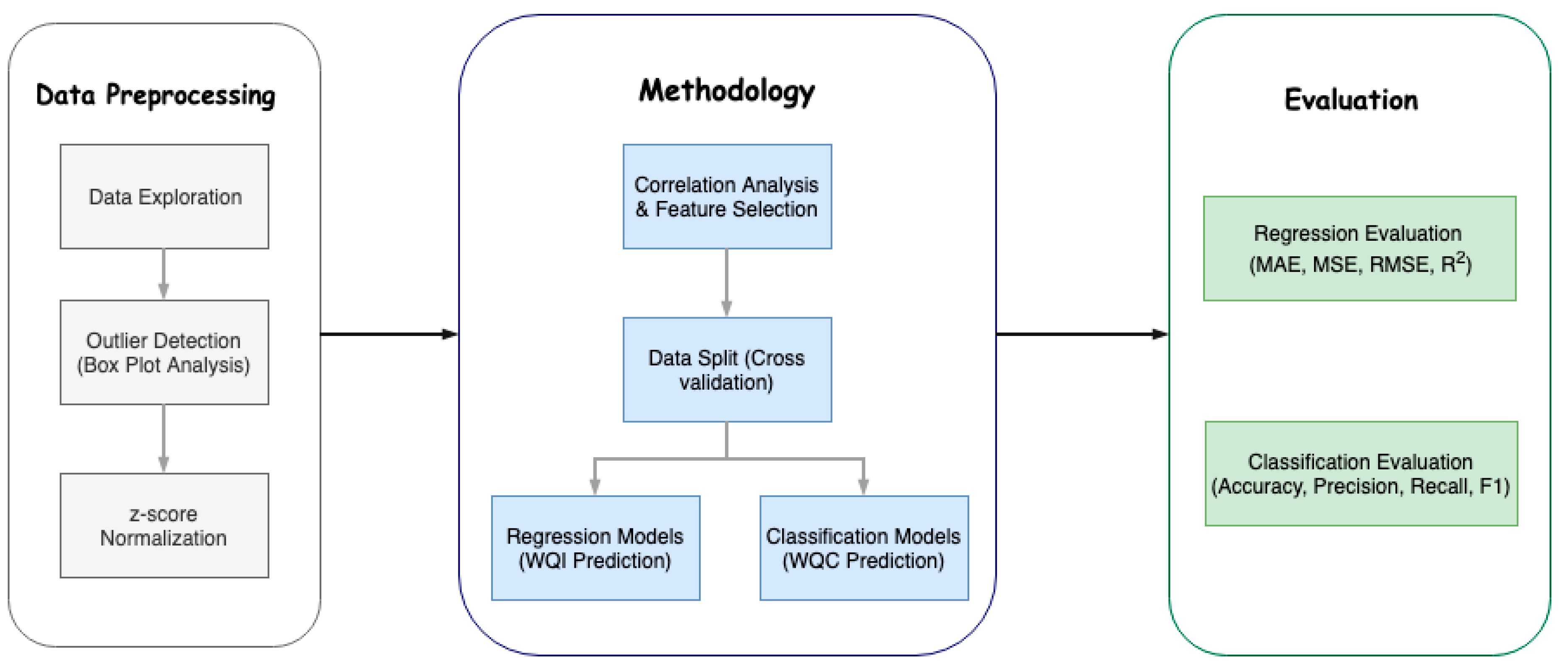
Most of the research either employed manual lab analysis, not estimating the water quality index standard, or used too many parameters to be efficient enough. The proposed methodology improves on these notions and the methodology being followed is depicted in Figure 1.
3. Data Preprocessing
The data used for this research was obtained from PCRWR and it was cleaned by performing a box plot analysis, discussed in this section. After the data were cleaned, they were normalized using q-value normalization to convert them to the range of 0–100 to calculate the WQI using six available parameters. Once the WQI was calculated, all original values were normalized using z-score, so they were on the same scale. The complete procedure is detailed next.
3.1. Data Collection
The dataset collected from PCRWR contained 663 samples from 13 different sources of Rawal Water Lake collected throughout 2009 to 2012. It contained 51 samples from each source and the 12 parameters listed in Table 1.
3.2. Boxplot Analysis and Outlier Detection
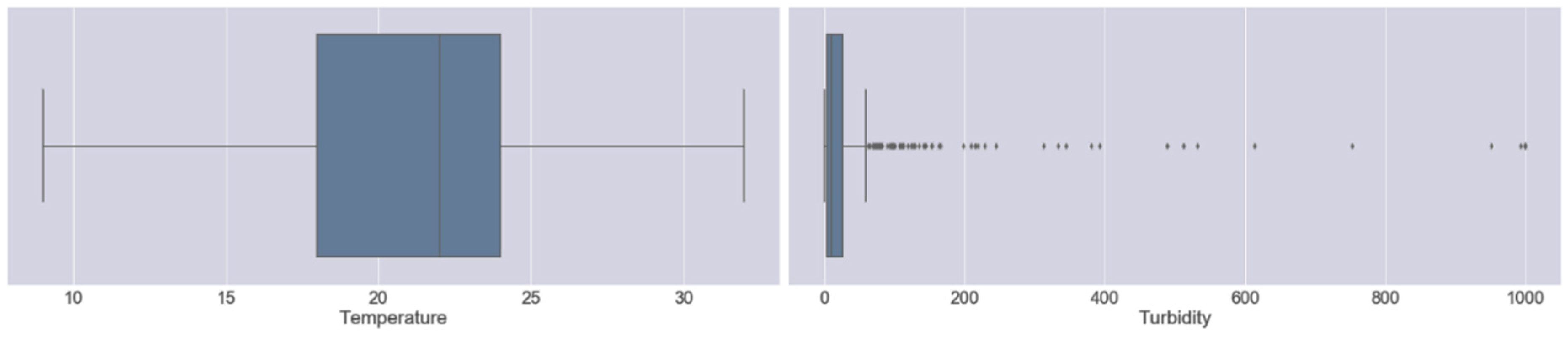
We chose boxplot analysis for outlier detection because most of the parameters varied enough and were on the higher end of the values, and a boxplot provides insightful visualization to decide outlier detection threshold values depending upon the problem domain. Boxplot analysis showed that most parameters lied outside the box, deeming outliers normal, so we adapted an upper cap strategy to filter out outliers. We recognized the parameter values that were very different from other values and replaced them with the max threshold value. We set the max threshold value as the parameter value that was just below the outlier values. For example, for turbidity, as reflected in Figure 2, we set the threshold value as the sample value, which was 753, and applied it to all values above 753, so that all the values that lied above 753 were assigned the value of 753. We repeated the same process with all the parameters and manually removed the outliers such as to not risk any data loss at all, given our limited dataset [4]. In addition, we were extremely lenient while choosing the upper threshold of parameters so as not to bias the dataset and just to loosely penalize the values that seemed way out of limits and unlikely to occur.
3.3. Water Qualiity Index (WQI)
Water quality index (WQI) is the singular measure that indicates the quality of water and it is calculated using various parameters that are truly reflective of the water’s quality. To conventionally calculate the WQI, nine water quality parameters are used, but if we did not have all of them, we could still estimate the water quality index with at least six defined parameters. We had five parameters, namely fecal coliform, pH, temperature, turbidity and total dissolved solids in our dataset. We also considered nitrites as the sixth parameter as the weight and relative importance of nitrites in the WQI calculation is stated to be equal to that of nitrates in multiple WQI studies [13,14,15]. Using these parameters and their assigned weightages, we calculated the WQI of each sample as reflected in Equation (1), where reflects the value of a parameter in the range of 0–100 and represents the weight of a particular parameter as listed in Table 2. WQI is fundamentally calculated by initially multiplying the q value of each parameter by its corresponding weight, adding them all up and then dividing the result by the sum of weights of the employed parameters [14,15].
3.4. Water Qulaity Class (WQC)
3.5. Q-Value Normalization
Q-value normalization was used to normalize the parameters, particularly the water quality parameters to fit them in the range of 0 to 100 for easier index calculation. Figure 3 shows the q-value charts for six of the water quality parameters. We used them to convert five of these parameters within the range of 0 to 100 [14,15]. For the sixth parameter, namely nitrites, due to unavailability of its q-value ranges, we used the WHO standards to distinctly convert them to the 0–100 range by means of a set of thresholds as follows: assigning 100 if its below 1, 80 if its below 2, 50 if its below 3 and 0 if its greater than 3, reflecting strict penalization. Once the values were q-normalized and were in the range of 0–100, they were used for calculating the WQI of the dataset using (1).
3.6. Z-Score Normalization
The z-score is a conventional standardization and normalization method that represents the number of standard deviations; a raw data point is above or below the population mean. It ideally lies between −3 and +3. It normalizes the dataset to the aforementioned scale to convert all the data with varying scales to the default scale.
To normalize the data using the z-score, we subtracted the mean of the population from a raw data point and divided it by the standard deviation, which gives a score ideally varying between −3 and +3; hence, reflecting how many standard deviations a point is above or below the mean as computed by Equation (2), where represents the value of a particular sample, represents the mean and represents the standard deviation [16].
3.7. Data Analysis
After all the data processing, for data analysis, several machine learning algorithms were employed to predict the WQI and WQC using the minimal number of parameters. Before applying a machine learning algorithm, there are some preliminary steps, like correlation analysis and data splitting, to prepare the data to be given as input to the actual machine learning algorithms.
3.7.1. Correlation Analysis
To find the dependent variables and to predict hard-to-estimate variables through easily attainable parameters, we performed correlation analysis to extract the possible relationships between the parameters. We used the most commonly used and effective correlation method, known as the Pearson correlation. We applied the Pearson correlation on the raw values of the parameters listed in Table 4 and applied it after normalizing the values through q-value normalization as explained in the subsequent section.
As the correlation chart in Table 4 indicates:
- Alkalinity (Alk) is highly correlated with hardness (CaCO3) and calcium (Ca).
- Hardness is highly correlated with alkalinity and calcium, and loosely correlated with pH.
- Conductance is highly correlated with total dissolved solids, chlorides and fecal coliform count, and loosely correlated with calcium and temperature.
- Calcium is highly correlated with alkalinity and hardness, while loosely correlated with TDS, chlorides, conductance and pH.
- TDS is highly correlated with conductance, chlorides and fecal coliform, and loosely correlated with calcium and temperature.
- Chlorides are highly correlated with conductance and TDS, and loosely correlated with temperature, calcium and fecal coliform.
- Fecal coliform is correlated with conductance and TDS, and loosely correlated with chlorides.
Now that we have listed the correlation analysis observations, we find that our predicting parameter WQI is correlated with seven parameters, namely temperature, turbidity, pH, hardness as CaCO3, conductance, total dissolved solids and fecal coliform count. We have to choose the minimal number of parameters to predict the WQI, in order to lower the cost of the system. The three parameters whose sensors are easily available, cost the lowest and contribute distinctly to the WQI are temperature, turbidity and pH, which deems them naturally selected. The other convenient parameter is total dissolved solids, whose sensor is also easily available and is correlated with conductance and fecal coliform count, which means selecting TDS would allow us to discard the other two parameters. We leave the remaining inconvenient parameter, hardness as CaCO3, out because it is not highly correlated comparatively and is not easy to acquire.
To conclude the correlation analysis, we selected four parameters for the prediction of WQI, namely, temperature, turbidity, pH and total dissolved solids. We initially just considered the first three parameters, given their low cost, and if needed, TDS will be included later to analyze its contribution to the accuracy.
3.7.2. Data Splitting–Cross Validation
The last step prior to applying the machine learning model is splitting the provided data in order to train the model, test it with a certain part of the data and compute the accuracy measures to establish the model’s performance. This research explores the cross validation data splitting technique.
Cross validation splits the data into k subsets and iterates over all the subsets, considering k-1 subsets as the training dataset and 1 subset as the testing dataset. This ensures an efficient split and use of proper and definitive data for training and testing. This is generally computationally expensive, given the iterations, but our research uses a small dataset, which is mostly the case with water quality datasets, making cross validation more suited for this problem. We split the data into k = 6 subsets and ran cross validation. Therefore, as the complete training set consists of 663 samples, we ensured at least 100 samples for each fold subset, including the test set.
3.7.3. Machine Learning Algorithms
We used both regression and classification algorithms. We used the regression algorithms to estimate the WQI and the classification algorithms to classify samples into the previously defined WQC. We used eight regression algorithms and 10 classification algorithms. The following algorithms were employed in our study:
(1) Multiple Linear Regression
Multiple linear regression is a form of linear regression used when there is more than one predicting variable at play. When there are multiple input variables, we use multiple linear regression to assess the input of each variable that affects the output, as reflected in Equation (3), where is the output for which machine learning has been applied to predict the value, is the observed value, is the slope on the observed value, and is the error term [17].
(2) Polynomial Regression
Polynomial regression is used when the relation between input and output variables is not linear and a little complex. We used a higher order of variables to capture the relation of input and output variables, which is not as linear. We used the order of two. Using a higher order of variables does carry the risk of overfitting, as reflected in Equation (4), where is the output for which machine learning has been applied to predict the value, is the observed value, is the fitting value, i is the number of parameters considered, k is the order of the polynomial equation, and is the error term or residuals of the ith predictor [18]. We used it with 2-degree polynomials with an order of C.
(3) Random Forest
Random forest is a model that uses multiple base models on subsets of the given data and makes decisions based on all the models. In random forest, the base model is a decision tree, carrying all the pros of a decision tree with the additional efficiency of using multiple models [19].
(4) Gradient Boosting Algorithm
This is the most contemporary algorithm used in most competitions. It uses an additive model that allows for optimization of differentiable loss function. We used it with a loss function of ‘ls’, a min_samples_split of 2 and a learning rate of 0.1 [20].
(5) Support Vector Machines
Support vector machines (SVMs) are mostly used for classification but they can be used for regression as well. Visualizing data points plotted on a plane, SVMs define a hyperplane between the classes and extend the margin in order to maximize the distinction between two classes, which results in fewer close miscalculations [21].
(6) Ridge Regression
Ridge regression works on the same principles as linear regression, it just adds a certain bias to negate the effect of large variances and to void the requirement of unbiased estimators. It penalizes the coefficients that are far from zero and minimizes the sum of squared residuals [22,23].
(7) Lasso Regression
Lasso regression works on the same principles as ridge regression, the only difference is how they penalize their coefficients that are off. Lasso penalizes the sum of absolute errors instead of the sum of squared coefficients [24].
(8) Elastic Net Regression
Elastic net regression combines the best of both ridge and lasso regression. It combines the method of penalties of both methods and minimizes the loss function [25].
(9) Neural Net/Multi-Layer Perceptrons (MLP)
Neural nets are loosely based on the structure of neurons. They contain multiple layers with interconnected nodes. They contain an input layer and output layer, and hidden layers in between these two mandatory layers. The input layer takes in the predicting parameters and the output layer shows the prediction based on the input. They iterate through each training data point and generalize the model by giving and updating the weight on each node of each layer. The trained model then uses those weights to decide what units to activate based on the input. Multi-layer perceptron (MLP) is a conventional model of neural net, which is mostly used for classification, but it can be used for regression as well [26]. We used it for classification with the configuration of (3, 7) running for a maximum of 200 epochs using ‘lbfgs’ solver.
(10) Gaussian Naïve Bayes
Naïve Bayes is a simple and a fast algorithm that works on the principle of Bayes theorem with the assumption that the probability of the presence of one feature is unrelated to the probability of the presence of the other feature [27].
(11) Logistic Regression
Logistic regression is a classification algorithm. It is based on the logistic function or the sigmoid function, hence the name. It is the most common algorithm used in the case of binary classification, but in our case we used multinomial logistic regression because there was more than two classes [28]. We used it with ‘warn’ solver and l2 penalty.
(12) Stochastic gradient descent
This iterative optimization algorithm minimizes the loss function iteratively to find the global optimum. In stochastic gradient descent, the sample selection is random [29].
(13) K Nearest Neighbor
The K nearest neighbor algorithm classifies by finding the given points nearest N neighbors and assigns the class of majority of n neighbors to it. In the case of a draw, one could employ different techniques to resolve it, e.g., increase n or add bias towards one class. K nearest neighbor is not recommended for large datasets because all the processing takes place while testing, and it iterates through the whole training data and computes nearest neighbors each time [30]. We used a n = 5 configuration for our model.
(14) Decision Tree
A decision tree is a simple self-explanatory algorithm, which can be used for both classification and regression. The decision tree, after training, makes decisions based on values of all the relevant input parameters. It uses entropy to select the root variable, and, based on this, it looks towards the other parameters’ values. It has all the parameter decisions arranged in a top-to-down tree and projects the decision based on different values of different parameters [31].
(15) Bagging Classifier
A bagging classifier fits multiple base classifiers on random subsets of data and then averages out their predictions to form the final prediction. It greatly helps out with the variance [32].
We used default values for the algorithms, except MLP, which uses a (3, 7) configuration.
4. Results
In this section, prior to discussing the results, we will describe different measures used to assess the accuracy of the applied machine learning algorithms.
4.1. Accuracy Measures
As mentioned earlier, this research employed two types of supervised machine learning algorithms, i.e., regression and classification. The results yielded by both types of algorithms were evaluated differently.
For regression, we used the following measures:
(1) Mean Absolute Error (MAE)
Mean absolute error (MAE) is a measure of accuracy for regression. It sums up absolute values of errors and divides them by the total number of values. It gives equal weight to each error value. The formula for calculating MAE is shown in Equation (5), where refers to the actual value, refers to the predicted value, and refers to the total number of samples considered [33].
(2) Mean Square Error (MSE)
Mean square error (MSE) is the sum of squares of errors divided by the total number of predicted values. This attributes greater weight to larger errors. This is particularly useful in problems where there needs to be a larger weight for larger errors. It is measured by Equation (6), where is the actual value, is the predicted value, and is the total number of samples considered [33].
(3) Root Mean Squared Error (RMSE)
Root mean squared error (RMSE) is just the square root of MSE and scales the values of MSE near to the ranges of observed values. It is estimated from Equation (7), where points to the actual value, points to the predicted value, and points to the total number of samples considered [33].
(4) R Squared Error (RSE)
R squared error (RSE), also known as the coefficient of determination, and often denoted as , determines the goodness of fit of the model. It particularly explains the amount of variance of the dependent variable that is explainable through the independent variable, as shown in Equation (8). Higher RSE values mean that the independent variables largely explain the variance of the dependent variable [34].
For classification, we used the following measures:
(1) Accuracy
Accuracy is the correct number of predictions made by the model over all the observed values. Accuracy is measured by Equation (9), where refers to true positive, refers to true negative, refers to false positive and refers to false negative [7,35].
(2) Precision
Precision is the proportion of correctly classified instances of a particular positive class out of the total classified instances of that class. Precision is calculated with the formula shown in Equation (10), where refers to true positive and refers to false positive [7,35,36].
(3) Recall
Recall is the proportion of instances of a particular positive class that were actually classified correctly. Recall is calculated with the formula shown in Equation (11), where refers to true positive and refers to false negative [7,35,36].
(4) F1 Score
As precision and recall, individually, do not cover all aspects of the accuracy, we took their harmonic mean to reflect the F1 score, as shown in Equation (12), which covers both aspects and reflects the overall accuracy measure better. It ranges between 0 and 1. The higher the score, the better the accuracy [7,35,36].
4.2. Results for Regression Algorithms
As water quality parameter sensors are expensive, this study aimed to use a minimal number of parameters with cheap sensors to predict water quality. Initially, we used four parameters, namely temperature, turbidity, pH and total dissolved solids. While employing the regression algorithms, we found gradient boosting, having a MAE of 1.9642, MSE of 7.2011, RMSE of 2.6835 and RSE of 0.7485, to be the most efficient algorithm, as shown in Table 5.
Following that, we tried to reduce more parameters, and so we decided to drop total dissolved solids, which is a little harder to acquire than the others. We found that the polynomial regression, with a MAE of 2.7273, MSE of 12.7307, and RMSE of 3.5680, to be the most efficient algorithm, although linear regression and gradient boosting had the best RSE values, with 0.5384 and 0.5051, respectively, as shown in Table 6. There was an increase in the overall error rate, but the increase was not alarming and still performed well within the limits, given the cost.
4.3. Results for Classification Algorithms
Using classification algorithms, we predicted water quality class (WQC), which was assigned to samples based on their pre calculated WQI. The same parameters, as in previous section, were used for classification as well. Initially, the same four parameters were considered. We found that MLP, in such a setting, performed better than the other algorithms, with an accuracy of 0.8507, precision of 0.5659, recall of 0.5640, and F1 score of 0.5649, as shown in Table 7.
In this section, we iterated through our study’s results and established that gradient boosting and polynomial regression performed better in predicting WQI, whereas MLP performed better in predicting WQC.
5. Discussion
Water Quality is conventionally calculated using water quality parameters, which are acquired through time consuming lab analysis. We explored alternative methods of machine learning to estimate it and found several studies employing them. These studies used more than 10 water quality parameters to predict WQI. Ahmad et al. [8] used 25 input parameters, Sakizadeh [9] used 16 parameters, Gazzaz et al. [4] used 23 input parameters in their methodology, and Rankovic et al. [12] used 10 input parameters, which is unsuitable for inexpensive real time systems. Whereas, our methodology employs only four water quality parameters to predict WQI, with a MAE of 1.96, and to predict water quality class with an accuracy of 85%. Our results make a base for an inexpensive real time water quality detection system, while other studies, although they use machine learning, use too many parameters to be incorporated in real time systems.
6. Conclusions and Future Work
Water is one of the most essential resources for survival and its quality is determined through WQI. Conventionally, to test water quality, one has to go through expensive and cumbersome lab analysis. This research explored an alternative method of machine learning to predict water quality using minimal and easily available water quality parameters. The data used to conduct the study were acquired from PCRWR and contained 663 samples from 12 different sources of Rawal Lake, Pakistan. A set of representative supervised machine learning algorithms were employed to estimate WQI. This showed that polynomial regression with a degree of 2, and gradient boosting, with a learning rate of 0.1, outperformed other regression algorithms by predicting WQI most efficiently, while MLP with a configuration of (3, 7) outperformed other classification algorithms by classifying WQC most efficiently.
In future works, we propose integrating the findings of this research in a large-scale IoT-based online monitoring system using only the sensors of the required parameters. The tested algorithms would predict the water quality immediately based on the real-time data fed from the IoT system. The proposed IoT system would employ the parameter sensors of pH, turbidity, temperature and TDS for parameter readings and communicate those readings using an Arduino microcontroller and ZigBee transceiver. It would identify poor quality water before it is released for consumption and alert concerned authorities. It will hopefully result in curtailment of people consuming poor quality water and consequently de-escalate harrowing diseases like typhoid and diarrhea. In this regard, the application of a prescriptive analysis from the expected values would lead to future facilities to support decision and policy makers.
Author Contributions
Conceptualization, R.M.; Data curation, H.A.; Formal analysis, U.A. and R.I.; Investigation, A.A.S.; Methodology, U.A.; Resources, R.M.; Supervision, R.M.; Validation, U.A. and R.M.; Writing—original draft, U.A.; Writing—review & editing, R.M., H.A., R.I. and J.G.-N.
Funding
This research received no external funding.
Conflicts of Interest
The authors declare no conflicts of interest.
References
- PCRWR. National Water Quality Monitoring Programme, Fifth Monitoring Report (2005–2006); Pakistan Council of Research in Water Resources Islamabad: Islamabad, Pakistan, 2007. Available online: http://www.pcrwr.gov.pk/Publications/Water%20Quality%20Reports/Water%20Quality%20Monitoring%20Report%202005-06.pdf (accessed on 23 August 2019).
- Mehmood, S.; Ahmad, A.; Ahmed, A.; Khalid, N.; Javed, T. Drinking Water Quality in Capital City of Pakistan. Open Access Sci. Rep. 2013, 2. [Google Scholar] [CrossRef]
- PCRWR. Water Quality of Filtration Plants, Monitoring Report; PCRWR: Islamabad, Pakistan, 2010. Available online: http://www.pcrwr.gov.pk/Publications/Water%20Quality%20Reports/FILTRTAION%20PLANTS%20REPOT-CDA.pdf (accessed on 23 August 2019).
- Gazzaz, N.M.; Yusoff, M.K.; Aris, A.Z.; Juahir, H.; Ramli, M.F. Artificial neural network modeling of the water quality index for Kinta River (Malaysia) using water quality variables as predictors. Mar. Pollut. Bull. 2012, 64, 2409–2420. [Google Scholar] [CrossRef]
- Daud, M.K.; Nafees, M.; Ali, S.; Rizwan, M.; Bajwa, R.A.; Shakoor, M.B.; Arshad, M.U.; Chatha, S.A.S.; Deeba, F.; Murad, W.; et al. Drinking water quality status and contamination in Pakistan. BioMed Res. Int. 2017, 2017, 7908183. [Google Scholar] [CrossRef]
- Alamgir, A.; Khan, M.N.A.; Hany; Shaukat, S.S.; Mehmood, K.; Ahmed, A.; Ali, S.J.; Ahmed, S. Public health quality of drinking water supply in Orangi town, Karachi, Pakistan. Bull. Environ. Pharmacol. Life Sci. 2015, 4, 88–94. [Google Scholar]
- Shafi, U.; Mumtaz, R.; Anwar, H.; Qamar, A.M.; Khurshid, H. Surface Water Pollution Detection using Internet of Things. In Proceedings of the 2018 15th International Conference on Smart Cities: Improving Quality of Life Using ICT & IoT (HONET-ICT), Islamabad, Pakistan, 8–10 October 2018; pp. 92–96. [Google Scholar]
- Ahmad, Z.; Rahim, N.; Bahadori, A.; Zhang, J. Improving water quality index prediction in Perak River basin Malaysia through a combination of multiple neural networks. Int. J. River Basin Manag. 2017, 15, 79–87. [Google Scholar] [CrossRef]
- Sakizadeh, M. Artificial intelligence for the prediction of water quality index in groundwater systems. Model. Earth Syst. Environ. 2016, 2, 8. [Google Scholar] [CrossRef]
- Abyaneh, H.Z. Evaluation of multivariate linear regression and artificial neural networks in prediction of water quality parameters. J. Environ. Health Sci. Eng. 2014, 12, 40. [Google Scholar] [CrossRef]
- Ali, M.; Qamar, A.M. Data analysis, quality indexing and prediction of water quality for the management of rawal watershed in Pakistan. In Proceedings of the Eighth International Conference on Digital Information Management (ICDIM 2013), Islamabad, Pakistan, 10–12 September 2013; pp. 108–113. [Google Scholar]
- Ranković, V.; Radulović, J.; Radojević, I.; Ostojić, A.; Čomić, L. Neural network modeling of dissolved oxygen in the Gruža reservoir, Serbia. Ecol. Model. 2010, 221, 1239–1244. [Google Scholar] [CrossRef]
- Kangabam, R.D.; Bhoominathan, S.D.; Kanagaraj, S.; Govindaraju, M. Development of a water quality index (WQI) for the Loktak Lake in India. Appl. Water Sci. 2017, 7, 2907–2918. [Google Scholar] [CrossRef] [Green Version]
- Thukral, A.; Bhardwaj, R.; Kaur, R. Water quality indices. Sat 2005, 1, 99. [Google Scholar]
- Srivastava, G.; Kumar, P. Water quality index with missing parameters. Int. J. Res. Eng. Technol. 2013, 2, 609–614. [Google Scholar]
- Jayalakshmi, T.; Santhakumaran, A. Statistical normalization and back propagation for classification. Int. J. Comput. Theory Eng. 2011, 3, 1793–8201. [Google Scholar]
- Amral, N.; Ozveren, C.; King, D. Short term load forecasting using multiple linear regression. In Proceedings of the 2007 42 nd International Universities Power Engineering Conference, Brighton, UK, 4–6 September 2007; pp. 1192–1198. [Google Scholar]
- Ostertagová, E. Modelling using polynomial regression. Procedia Eng. 2012, 48, 500–506. [Google Scholar] [CrossRef]
- Liaw, A.; Wiener, M. Classification and regression by randomForest. R News 2002, 2, 18–22. [Google Scholar]
- Friedman, J.H. Stochastic gradient boosting. Comput. Stat. Data Anal. 2002, 38, 367–378. [Google Scholar] [CrossRef]
- Tong, S.; Koller, D. Support vector machine active learning with applications to text classification. J. Mach. Learn. Res. 2001, 2, 45–66. [Google Scholar]
- Hoerl, A.E.; Kennard, R.W. Ridge regression: Biased estimation for nonorthogonal problems. Technometrics 1970, 12, 55–67. [Google Scholar] [CrossRef]
- Zhang, Y.; Duchi, J.; Wainwright, M. Divide and conquer kernel ridge regression: A distributed algorithm with minimax optimal rates. J. Mach. Learn. Res. 2015, 16, 3299–3340. [Google Scholar]
- Tibshirani, R. Regression shrinkage and selection via the lasso. J. R. Stat. Soc. Ser. B 1996, 58, 267–288. [Google Scholar] [CrossRef]
- Zou, H.; Hastie, T. Regression shrinkage and selection via the elastic net, with applications to microarrays. J. R. Stat. Soc. Ser. B 2003, 67, 301–320. [Google Scholar] [CrossRef]
- Günther, F.; Fritsch, S. Neuralnet: Training of neural networks. R J. 2010, 2, 30–38. [Google Scholar] [CrossRef]
- Zhang, H. The optimality of naive Bayes. AA 2004, 1, 3. [Google Scholar]
- Hosmer, D.W., Jr.; Lemeshow, S.; Sturdivant, R.X. Applied Logistic Regression; John Wiley Sons: Hoboken, NJ, USA, 2013. [Google Scholar]
- Bottou, L. Large-scale machine learning with stochastic gradient descent. In Proceedings of the COMPSTAT’2010, Paris, France, 22–27August 2010; pp. 177–186. [Google Scholar]
- Beyer, K.; Goldstein, J.; Ramakrishnan, R.; Shaft, U. When is “nearest neighbor” meaningful? In Proceedings of the International Conference on Database Theory, Jerusalem, Israel, 10–12 January 1999; pp. 217–235. [Google Scholar]
- Quinlan, J.R. Decision trees and decision-making. IEEE Trans. Syst. Man Cybern. 1990, 20, 339–346. [Google Scholar] [CrossRef]
- Breiman, L. Bagging predictors. Mach. Learn. 1996, 24, 123–140. [Google Scholar] [CrossRef] [Green Version]
- Willmott, C.J.; Matsuura, K. Advantages of the mean absolute error (MAE) over the root mean square error (RMSE) in assessing average model performance. Clim. Res. 2005, 30, 79–82. [Google Scholar] [CrossRef]
- Menard, S. Coefficients of determination for multiple logistic regression analysis. Am. Stat. 2000, 54, 17–24. [Google Scholar]
- Sokolova, M.; Japkowicz, N.; Szpakowicz, S. Beyond accuracy, F-score and ROC: A family of discriminant measures for performance evaluation. In Proceedings of the Australasian Joint Conference on Artificial Intelligence, Hobart, Australia, 4–8 December 2006; pp. 1015–1021. [Google Scholar]
- Goutte, C.; Gaussier, E. A probabilistic interpretation of precision, recall and F-score, with implication for evaluation. In Proceedings of the European Conference on Information Retrieval, Santiago de Compostela, Spain, 21–23 March 2005; pp. 345–359. [Google Scholar]
Figure 1.
Methodology flow.

Figure 2.
Outlier detection using box plot analysis.

Figure 3.
Q-value normalization range charts.


Table 1.
Parameters along with their “WHO” standard limits [11].
Table 1.
Parameters along with their “WHO” standard limits [11].
| Parameter | WHO Limits |
|---|---|
| Alkalinity | 500 mg/L |
| Appearance | Clear |
| Calcium | 200 mg/L |
| Chlorides | 200 mg/L |
| Conductance | 2000 µS/cm |
| Fecal Coliforms | Nil Colonies/100 mL |
| Hardness as CaCO3 | 500 mg/L |
| Nitrite as NO2− | <1 mg/L |
| pH | 6.5–8.5 |
| Temperature | °C |
| Total Dissolved Solids | 1000 mg/L |
| Turbidity | 5 NTU |
| Weighing Factor | Weight |
|---|---|
| pH | 0.11 |
| Temperature | 0.10 |
| Turbidity | 0.08 |
| Total Dissolved Values | 0.07 |
| Nitrates | 0.10 |
| Fecal Coliform | 0.16 |
| Water Quality Index Range | Class |
|---|---|
| 0–25 | Very bad |
| 25–50 | Bad |
| 50–70 | Medium |
| 70–90 | Good |
| 90–100 | Excellent |
Table 4.
Correlation Analysis Chart.
| Temp | Turb | pH | Alk | CaCO3 | Cond | Ca | TDS | Cl | NO2 | FC | WQI | |
|---|---|---|---|---|---|---|---|---|---|---|---|---|
| Temp | 1.000 | 0.103 | 0.005 | −0.193 | −0.288 | 0.266 | −0.150 | 0.274 | 0.293 | −0.154 | 0.194 | −0.467 |
| Turb | 0.103 | 1.000 | −0.0886 | −0.093 | −0.146 | 0.048 | −0.122 | 0.042 | 0.037 | 0.0002 | 0.037 | −0.354 |
| pH | 0.005 | −0.088 | 1.000 | −0.177 | −0.278 | −0.065 | −0.236 | −0.060 | −0.149 | 0.167 | 0.054 | −0.431 |
| Alk | −0.193 | −0.092 | −0.177 | 1.000 | 0.462 | 0.011 | 0.444 | 0.012 | 0.061 | 0.046 | 0.013 | 0.223 |
| CaCO3 | −0.288 | −0.146 | −0.278 | 0.462 | 1.000 | 0.068 | 0.637 | 0.060 | 0.135 | 0.078 | 0.016 | 0.360 |
| Cond | 0.266 | 0.048 | −0.064 | 0.011 | 0.068 | 1.000 | 0.225 | 0.973 | 0.780 | 0.100 | 0.456 | −0.370 |
| Ca | −0.150 | −0.122 | −0.236 | 0.444 | 0.637 | 0.225 | 1.000 | 0.219 | 0.262 | 0.124 | 0.113 | 0.188 |
| TDS | 0.273 | 0.041 | −0.060 | 0.012 | 0.060 | 0.974 | 0.219 | 1.000 | 0.765 | 0.095 | 0.454 | −0.381 |
| Cl | 0.292 | 0.037 | −0.149 | 0.061 | 0.135 | 0.780 | 0.262 | 0.765 | 1.000 | 0.036 | 0.353 | −0.274 |
| NO2 | −0.154 | 0.0002 | 0.167 | 0.046 | 0.078 | 0.100 | 0.124 | 0.095 | 0.036 | 1.000 | 0.193 | −0.209 |
| FC | 0.194 | 0.037 | 0.053 | 0.012 | 0.016 | 0.456 | 0.113 | 0.454 | 0.353 | 0.193 | 1.000 | −0.421 |
| WQI | −0.467 | −0.354 | −0.431 | 0.223 | 0.360 | −0.370 | 0.188 | −0.381 | −0.274 | −0.209 | −0.421 | 1.000 |
Table 5.
Regression results using four parameters.
| Algorithm | MAE | MSE | RMSE | R Squared |
|---|---|---|---|---|
| Linear Regression | 2.6312 | 11.7550 | 3.4286 | 0.6573 |
| Polynomial Regression | 2.0037 | 7.9467 | 2.8190 | 0.7134 |
| Random Forest | 2.3053 | 9.5669 | 3.0930 | 0.6705 |
| Gradient Boosting | 1.9642 | 7.2011 | 2.6835 | 0.7485 |
| SVM | 2.4373 | 10.6333 | 3.2609 | 0.3458 |
| Ridge Regression | 2.6323 | 11.7500 | 3.4278 | 0.4971 |
| Lasso Regression | 3.5850 | 20.1185 | 4.4854 | −2.9327 |
| Elastic Net Regression | 3.6595 | 20.9698 | 4.5793 | −4.0050 |
Table 6.
Regression results using three parameters.
| Algorithm | MAE | MSE | RMSE | R Squared |
|---|---|---|---|---|
| Linear Regression | 3.1375 | 15.8321 | 3.9790 | 0.5384 |
| Polynomial Regression | 2.7273 | 12.7307 | 3.5680 | 0.4851 |
| Random Forest | 3.0404 | 15.2473 | 3.9048 | 0.4107 |
| Gradient Boosting | 2.8060 | 13.2710 | 3.6429 | 0.5051 |
| SVM | 2.8252 | 13.8546 | 3.7222 | 0.1546 |
| Ridge Regression | 3.1386 | 15.8327 | 3.9790 | 0.2031 |
| Lasso Regression | 3.8800 | 22.9966 | 4.7955 | −3.6636 |
| Elastic Net Regression | 3.9697 | 24.0678 | 4.9059 | −5.5210 |
Table 7.
Classification results using four parameters.
| Algorithm | Accuracy | Precision | Recall | F1 Score |
|---|---|---|---|---|
| MLP | 0.8507 | 0.5659 | 0.5640 | 0.5649 |
| Guassian Naïve Bayes | 0.7843 | 0.4964 | 0.5491 | 0.5025 |
| Logistic Regression | 0.8401 | 0.5520 | 0.5594 | 0.5548 |
| Stochastic Gradient Descent | 0.8205 | 0.5473 | 0.5424 | 0.5443 |
| KNN | 0.7270 | 0.4734 | 0.4783 | 0.4750 |
| Decision Tree | 0.7949 | 0.5298 | 0.5250 | 0.5268 |
| Random Forest | 0.7587 | 0.5063 | 0.5011 | 0.5027 |
| SVM | 0.7979 | 0.5187 | 0.5327 | 0.5228 |
| Gradient Boosting Classifier | 0.8130 | 0.5375 | 0.5376 | 0.5376 |
| Bagging Classifier | 0.8100 | 0.5410 | 0.5354 | 0.5374 |
© 2019 by the authors. Licensee MDPI, Basel, Switzerland. This article is an open access article distributed under the terms and conditions of the Creative Commons Attribution (CC BY) license (http://creativecommons.org/licenses/by/4.0/).
Share and Cite
MDPI and ACS Style
Ahmed, U.; Mumtaz, R.; Anwar, H.; Shah, A.A.; Irfan, R.; García-Nieto, J. Efficient Water Quality Prediction Using Supervised Machine Learning. Water 2019, 11, 2210. https://doi.org/10.3390/w11112210
AMA Style
Ahmed U, Mumtaz R, Anwar H, Shah AA, Irfan R, García-Nieto J. Efficient Water Quality Prediction Using Supervised Machine Learning. Water. 2019; 11(11):2210. https://doi.org/10.3390/w11112210
Chicago/Turabian StyleAhmed, Umair, Rafia Mumtaz, Hirra Anwar, Asad A. Shah, Rabia Irfan, and José García-Nieto. 2019. "Efficient Water Quality Prediction Using Supervised Machine Learning" Water 11, no. 11: 2210. https://doi.org/10.3390/w11112210
Note that from the first issue of 2016, this journal uses article numbers instead of page numbers. See further details here.