Terrestrial Laser Scanning for the Detection of Coarse Grain Size Movement in a Mountain Riverbed


1
Institute of Geodesy and Geoinformatics, Wrocław University of Environmental and Life Sciences, Grunwaldzka 53, 50-357 Wrocław, Poland
2
Institute of Geography and Regional Development, University of Wroclaw, pl. Uniwersytecki 1, 50-137 Wrocław, Poland
*
Author to whom correspondence should be addressed.
Water 2019, 11(11), 2199; https://doi.org/10.3390/w11112199
Submission received: 6 August 2019
/
Revised: 17 October 2019
/
Accepted: 17 October 2019
/
Published: 23 October 2019
(This article belongs to the Special Issue Close-Range Remote Sensing and Modern Field Measurements in Fluvial Geomorphology)
Abstract
:Fluvial transport is a natural process that shapes riverbeds and the surrounding terrain surface, particularly in mountainous areas. Since the traditional techniques used for fluvial transport investigation provide only limited information about the bed load transport, recently, laser scanning technology has been increasingly incorporated into research to investigate this issue in depth. In this study, a terrestrial laser scanning technique was used to investigate the transport of individual boulders. The measurements were carried out annually from 2011 to 2016 on the Łomniczka River, which is a medium-sized mountain stream. The main goal of this research was to detect and determine displacements of the biggest particles in the mountain riverbed. The methodology was divided into two steps. First, the change zones were detected using two strategies. The first strategy was based on differential digital elevation model (DEM) creation and the second involved the calculation of differences between point clouds instead of DEMs. The experiments show that the second strategy was more efficient. In the second step, the displacements of the boulders were determined based on the detected areas of change. Using the proposed methodology, displacements for individual stones in each year were determined. Most of the changes took place in 2012–2014, which correlates well with the hydrological observations. During the six-year period, movements of individual particles with diameters less than 0.8 m were observed. Maximal displacements in the observed period reached 3 m. Therefore, it is possible to determine both vertical and horizontal displacement in the riverbed using multitemporal TLS.
1. Introduction
Fluvial transport is a natural surface process that shapes the riverbed and surrounding terrain surface, particularly in mountainous areas. The understanding of sediment transport is important for many applications related to watershed management, such as changes in flow regime or channel restoration [1]. Knowledge about the ability of the river to transport a specified volume of bed load is also an essential task in natural hazard investigations, engineering design, flood control, and ecology [2].
The dynamic changes in a river channel caused by fluvial transport are traditionally measured using sediment traps (e.g., [3,4,5]) or tracers (e.g., [6,7,8,9,10,11]), or are roughly estimated by means of bed load transport equations (e.g., [12,13,14,15]). However, none of these techniques ensure full information about the bed load transport, since they are limited to the calculation of the total volume of transported rock material or short-term movement detection. The spatial distribution of transported sediments along the watercourse remains unknown. This information can be potentially supplemented by introducing remote sensing techniques. In particular, terrestrial laser scanning (TLS) is a new possibility in this context.
TLS is an active remote sensing technique used for the acquisition of high-density 3D geometry information about anthropogenic and natural surfaces. The TLS technique is used in a wide range of applications, such as topographic mapping, geological surveys, engineering practice, cultural heritage restoration, forest inventory, and many other environmental applications [16]. Recently, terrestrial laser scanning has also been applied to determine the structure and topography of river channels and their dynamic changes due to fluvial processes, especially in mountain rivers [17,18,19,20]. TLS data were used to determine the roughness parameters of the dry gravel in riverbeds [21,22]. Similarly, in [23], the gravel structure was described by the statistical parameters obtained from a detailed digital elevation model (DEM) that was interpolated from a TLS point cloud. In this case, DEM was limited to the part of the gravel surface that was visible above the water level. An exposed riverbed surface mapped with a TLS is the subject of the investigation in [24], aiming at finding the links between spatially distributed pathways of gravel transportation, hydraulic patterns, and morphological changes in a shallow river.
Laser scanning is also commonly used in fluvial applications to create DEMs and calculate the difference between two of them (DoD = DEM of difference) to describe the river channel topography at two different moments, e.g., [18,19,20]. The main drawback of this procedure is that it allows for the detection of topographic changes only in the vertical direction. This means that the differential DEM provides only limited information about the fluvial transport since the information about long-term spatial distribution of bed load along the watercourse remains unknown.
To fill this gap, the DoD method may be supplemented with detection and measurement of horizontal direction movement of sediments. Due to the complex nature of the fluvial transport, horizontal movement can only be estimated for a limited number of boulders that can be unambiguously identified in the point cloud data [25]. A similar approach was proposed by the authors of [26] to investigate the correlation of fluvial transport and the thickness of snow cover in a subarctic river for the short period of one year.
Despite the fact that a need for the determination of the displacement vector for each individual stone was indicated in [26], no more investigations have been undertaken. Therefore, the main goal of this research was to detect and measure the 3D displacement of boulders in the riverbed. The additional novelty of this study lies in the detection of change zones by analyzing the differential point cloud instead of the most commonly used method in fluvial studies: the DoD method.
This paper presents the results of fluvial transport monitoring in the mountain river channel, executed with terrestrial laser scanning in 2011–2016. Monitoring was performed for the Łomniczka River, which, in contrast to research areas previously reported on in the literature, is steeply inclined and characterized by the high complexity of the riverbed structure and the close presence of the surrounding vegetation.
This paper is structured as follows: in Section 2, four aspects are presented. First, the study area is characterized in both morphological and hydrological aspects. Next, the measurement campaign is characterized. Then, two strategies for change zone detection are introduced. Finally, the method of 3D movement detection is explained. Section 3 involves the results of the evaluation of the proposed methodology on the simulated dataset, shows the application of the two proposed strategies for detection of change zones, describes the method of 3D movement vectors calculation, and gives a discussion of the results obtained, the limitations of the proposed method, and potential alternatives to TLS. Section 4 presents the conclusions and provides a scope for future work.
2. Materials and Methods
2.1. Study Area
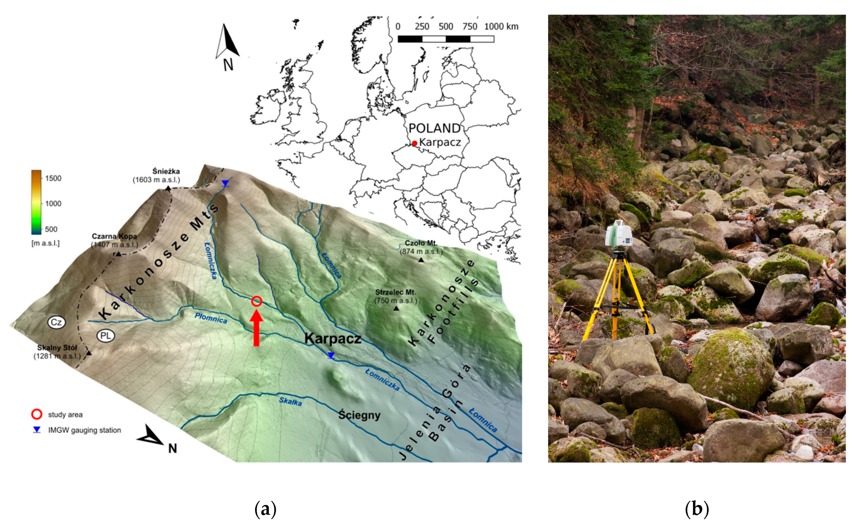
The Łomniczka River is a typical medium-sized mountain stream located on the northern slope of the Karkonosze Mountains—the highest mountain range of the Sudetes (Figure 1). This 8.7-km-long river is in the Baltic Sea catchment, whose spring is located at an altitude of 1402 m above sea level. The Łomniczka River is not hydrologically monitored, but some measurements were carried out periodically by the Polish Institute of Meteorology and Water Management (IMGW) in two water-gauge cross sections: in the upper course of the river and in Karpacz [27]. The hydrological statistics of Łomniczka River are summarized in Table 1.
A distinctive feature of the Łomniczka River is the high variability of flows throughout the year [28]. The highest flows occur in April, May, and July. These are conditioned by
- the spring thaw, often affected by rainfalls in April;
- the precipitation power falling shortly after the thaw in slightly lower parts of the mountains and the snow cover melting in the higher parts during May;
- heavy summer rainfall in July.
The lowest flow and water level occur during autumn (September, October) and winter (February). The summer floods of the river may be short-term and rapid after storms or last longer as a result of prolonged regional scattered rainfall [29]. During these floods, increased bed load transport occurs, including large particles, such as cobbles (64–256 mm) or boulders (diameter over 256 mm).
Continuous hydrological monitoring was carried out on the Łomnica River, into which the investigated river flows. Based on data collected at a water gauge station, it is clear that during the measurement period (2011–2016), no extreme flood events were recorded in the region. The highest water levels were recorded each summer after storms and during the spring thaw from March to May. The largest flow of water of the Łomnica River was recorded on 25 June 2013 and was equal to 56.2 m3 s−1, whereas the average flow rate for this indicator was equal to 0.58 m3 s−1 and the average flow was equal to 20.4 m3 s−1 [27]. This spate is almost double the value of flows recorded in other years of observation.
The study site includes a steeply inclined section of the riverbed (the local slope of the channel longitudinal section is over 133‰), with a length of about 30 m, where large boulders and blocks are the main components of the bed load. The section is located within a Pleistocene alluvial fan at the foot of a fault-generated escarpment. The area selection was based on several reasons. First, large particles are present in the riverbed, thus it was possible to get a sufficiently large test set. Second, there is a low water level and low flow in this river during autumn, which enables the measurement of lower parts of stones. For instance, on 24 October 2017, the flow was equal to 0.02 m3 s−1. Moreover, during the spring, there is a high water flow that is able to move a large mass of bed load. Finally, despite the relatively good recognition of flow conditions due to long-term hydrological measurements conducted on major rivers, knowledge about the fluvial transport in the Sudetes area is relatively poor.
2.2. Terrestrial Laser Scanning
A common issue with mapping a riverbed using the TLS technique is the deteriorated and limited propagation of the laser beam through the water, which is most significant in the case of the near-infrared lasers commonly used in terrestrial scanners. For this reason, most of the investigations were restricted to the part of the river channel that is exposed above the water surface. In some conditions, through-water TLS data acquisition is possible. The use of a green wavelength laser allows for obtaining the reflection from the bottom of the riverbed; however, the quality of the obtained point clouds was decreased due to refraction. To reduce this effect, the authors of [30] proposed corrections for through-water TLS measurements of gravel riverbeds.
To overcome some shortcomings of the use of TLS in fluvial geomorphology studies, a protocol for laser scanning was proposed in [31]. This protocol describes the field and processing techniques required for oblique laser scanning of the riverbed. Although many of the reported suggestions are essential (i.e., to select the locations of a laser scanner that enable the minimization of the shadowing effect), others are less critical due to the development of scanners and processing algorithms, as well as the investigation object and goal (i.e., to repeat scans from the same location in order to densify the point cloud).
The limitations of TLS use in fluvial applications were overcome in this study thanks to:
- The goal of the monitoring: Since the transportation of boulders happens occasionally during high flow, scanning campaigns are not required to be executed at constant cycles and can be performed with a longer break period, depending on the flow size.
- The season of the investigation: During autumn, the bed of the Łomniczka River stays almost dry. This presents the perfect conditions for scanning since all boulders are almost completely exposed during that time.
For these reasons, the measurements were carried out annually during the autumn in 2011–2016. The data were collected using two models of laser scanners: Leica ScanStation C10 C10 (Leica Geosystems AG, Glattbrugg, Switzerland) for data acquired in 2011–2014 and Leica ScanStation P20 C10 (Leica Geosystems AG, Glattbrugg, Switzerland) for data collected in 2014–2016. In 2014, both scanners were used for comparison purposes. The most important parameters of these scanners are compared in Table 2.
Measurements were taken from two positions: the first was located at the beginning of the chosen section, and the second was placed roughly in the middle of the test site (Figure 2). Both were positioned far above the scanned surface. This enabled better reproduction of the shape of individual particles and minimization of the “shadowing effect.” However, due to the complexity of the area around the river, it was not possible to add a third scanner position, which would allow the shadowing effect (Figure 3) to be eliminated.
A set of three evenly distributed targets was established in order to co-register and georeference two point clouds. For a leveled scanner (as executed in this study), only two targets are necessary to register two point clouds; any additional target increases the registration reliability. The position of each warp point was selected outside of the changing area and measured with centimeter-level accuracy using land surveying techniques. During data acquisition, RGB images were collected by the scanner, resulting in the true-color point cloud.
All the measurements were carried out with the greatest possible methodological compatibility in order to assure the comparability of the data collected in different years. These similarities included the same season of scanning, a nearly identical position of the scanner in each campaign, the same scanning parameters, reference to the same warp points, and the same coordinate system.
The registration and transformation of scans were executed using Leica Cyclone C10 (Leica Geosystems AG, Glattbrugg, Switzerland) software. Very high registration and georeferencing accuracies were achieved (Table 3).
2.3. Detection of Change Zones
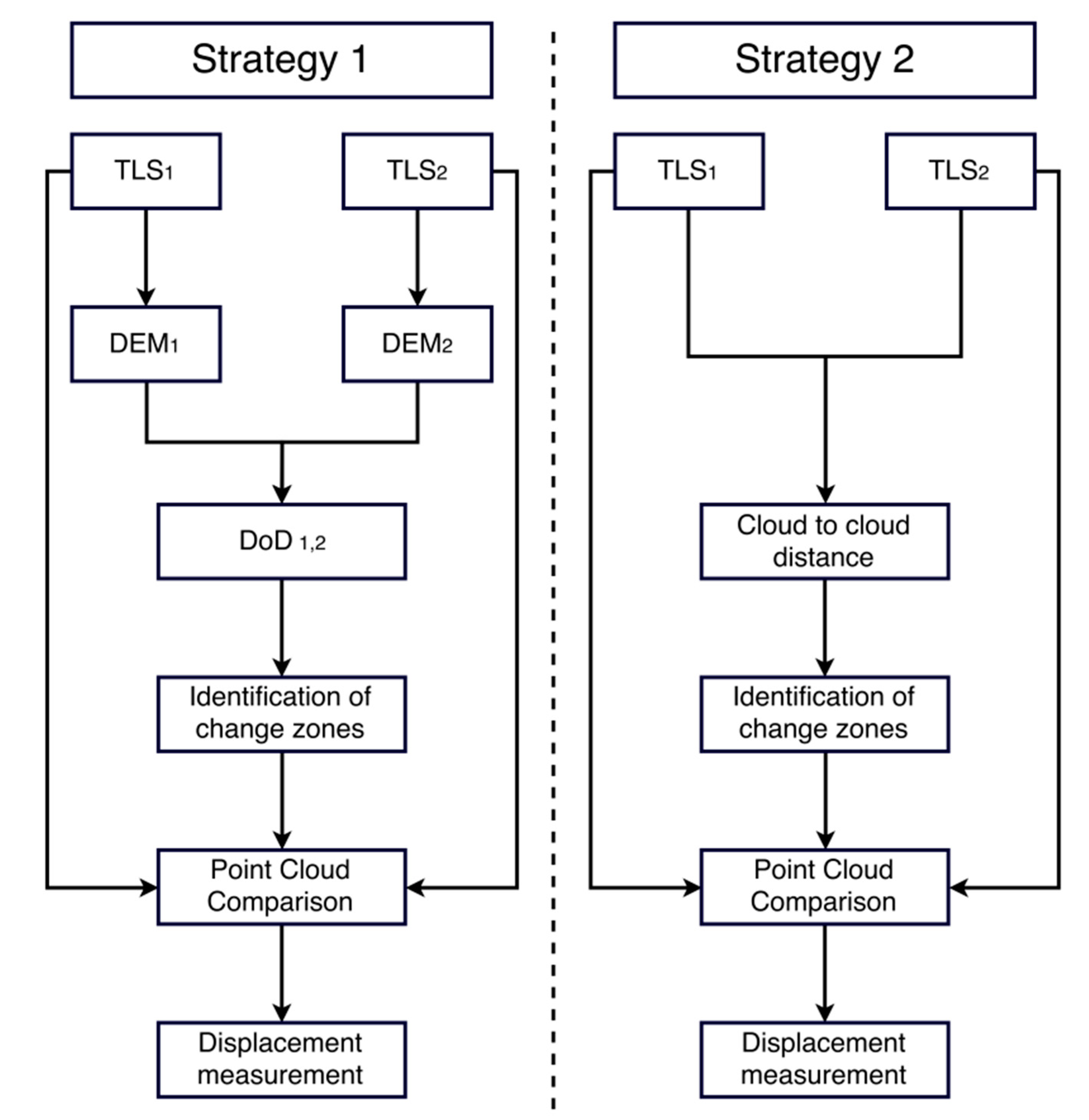
The determination of 3D displacement vectors proceeded in two stages. First, the change detection method was applied to narrow down the search area, then the identification of corresponding objects was performed (Section 3.2.3). In the first step, two strategies were investigated (Figure 4).
The basis of the first strategy was to use DEM of difference (DoD) to detect vertical changes in the riverbed. This method is widely used in geomorphological studies, e.g., [20,32,33]. The DoD product was acquired as a result of a two-step process. First, the point cloud was gridded to calculate a single value for each cell, which results in DEM creation. Then, the values from the corresponding cells of two DEMs were subtracted to obtain a DEM of difference. Although the algorithm is simple, it causes several problems, especially in the riverine areas. First, there are gaps in the point cloud caused by the “shadowing effect” or absorbance of the radiation by the water. This effect is a very common phenomenon and is impossible to remove due to the nature of the investigated object and the specificity of the research technique. Thus, the interpolation of the defining artificial value, such as the minimum or maximum value in the area for empty cells of DEM, is needed. However, this procedure can significantly disturb the results, causing false indications of changed areas. Another solution increases the size of a cell, but the shape of individual stones could be lost. Second, smaller particles, such as gravel grains (2–4 mm), may fill the gaps created by transporting larger stones to a new place. As a result, there may be underestimation or overestimation of the volume of material that was transported. Finally, the laser scanning data obtained for riverine areas are characterized by a high noise level, caused by reflections from vegetation or fine materials floating on the water surface. Taking into account all of the above problems, a more robust method of determining vertical changes in the riverbed should be developed.
Therefore, the second strategy was to calculate distances between point clouds based on the algorithm implemented in CloudCompare (http://www.cloudcompare.org) software [34]. The algorithm represents the distances as three components of the translation vector between corresponding points in the reference and compared point clouds. This procedure relies on the standard method of picking the corresponding points. First, for each point of the compared cloud, the algorithm finds the nearest point in the reference point cloud. Then, the Euclidean distance between these points is calculated. Displacements computed by this algorithm do not represent the real stone shift. This happens because, for each point in the considered point cloud, the distance is calculated to the closest point in the referenced cloud, instead of its equivalent, located at the same place on the stone. Taking this fact into consideration, in Strategy 2, only the vertical distance between point clouds was used to detect the change zones.
2.4. 3D Displacement Determination
Regardless of the chosen strategy, the obtained results only enabled us to depict places where vertical change occurred; there is no possibility of tracking the particle movement. The tracking can be done by a comparison of the point clouds acquired during different measurement campaigns. The comparison was based on previously identified change zones, particles size, and geometry. The identified change zones help to limit the search area in which to look for the displacement of individual particle. The displacement vectors should be calculated between points that represent the same objects.
The automatic methods of measuring displacements of stones in point clouds are extremely difficult to accomplish. Generally, a stone can be not only displaced but also rotated in 3D space, causing different parts of the stone surface to be scanned in different data acquisition campaigns. As a result, the identification of corresponding stones and the determination of the displacement vectors of individual stones between two following years have to be performed manually. For this reason, differential point clouds were visualized together with the merged point clouds obtained during the analyzed years. Insignificant changes were removed from the differential point cloud using a thresholding method. According to this method, the change is labeled as significant when its value exceeds a specified threshold value. The threshold value corresponds with the size of particles, whose movement will be tracked. The statistically computed threshold may create confusion when there is no movement in the test area. As a result, this would lead to ambiguous identification of change zones.
2.5. Synthetic Test
The synthetic dataset was acquired in order to validate the proposed methodology. The data were registered using the same laser scanner as in the case of real-world dataset Leica ScanStation P20 (Leica Geosystems AG, Glattbrugg, Switzerland). The measurements were taken from four positions. The obtained data were coregistered and georeferenced based on three targets whose coordinates were measured with centimeter-level accuracy. Then, 19 particles were randomly selected, marked with numbers, and displaced. After that, the second-epoch dataset was acquired using the laser scanner.
The displacements were found manually, based on the proposed methodology. First, the distances between the point clouds were calculated and projected on the joint point clouds. The change zones were obtained by thresholding the previously calculated distances. Then, the corresponding particles in both point clouds were found. For each particle, the movement distance between the scanning epochs was calculated.
The verification of the detected type of movement and the measured distances was performed based on an independent technique—photogrammetry. A set of 180 images was taken manually along two lines using a Nikon D800 (Nikon Corporation, Shinagawa, Tokyo, Japan) RGB camera equipped with a Nikon Nikkor (Nikon Corporation, Shinagawa, Tokyo, Japan) lens. Images in each line were taken three times in order to collect perpendicular and oblique (at two different angles) images with respect to the ground. This allowed for the reduction of occluded areas and increased image overlap. The average size of one pixel of the image on the ground was equal to about 1 mm. Local coordinates of 10 ground control points (GCPs), distributed on the whole test site and marked with special targets (Figure 5), were determined by total station measurements with an accuracy better than 1 cm. After the marked particles were displaced, second-epoch image data were acquired with the same parameters as in the first epoch. For both epochs, images were georeferenced using control points and a dense point cloud was calculated. The achieved image block adjustment accuracy was equal to 1 cm. Based on the point cloud, an orthomosaic with a resolution of 1 mm and a DEM with a resolution of 1.6 mm were generated using Agisoft Metashape (Agisoft LLC, St. Petersburg, Russia) software.
The reference displacements were found manually based on numbers written on the moved particles (Figure 5). Since the numbers were visible in the orthomosaic, the distance could be calculated between the same characteristic points of individual rocks in two scanning epochs. The characteristic points were chosen as easily recognizable parts of the number written on a particle. The 2D coordinates were acquired from the orthomosaic and the height was obtained from DEM.
3. Results and Discussion
3.1. Synthetic Test
First, the data collected using RGB camera were analyzed. Each particle that was marked with a number was found at the orthomosaic acquired in both epochs and the coordinates of its characteristic point were obtained. Then, the distances between the corresponding particles in different measurement epochs were calculated, taking into consideration both planar coordinates and height.
Secondly, the data collected using terrestrial laser scanning were analyzed. The corresponding particles in different measurement epochs were found manually based on differential point clouds. Then the distances between the particles were manually designated. Similar to the real-world example, a map representing the movement of individual particles was prepared (Figure 6).
When the distances for both techniques were calculated, the comparison of the results was executed. First, a qualitative analysis of the results was performed.
During the experiment, three types of possible movement situations were taken into account:
- 15 particles were moved on different distances and directions (the movement included both translation and rotation);
- three new particles were placed in the test area for the second-epoch measurement;
- one particle was removed from the test area after the first-epoch measurement.
The results obtained using TLS data were manually compared to the results obtained from image data to validate the capability of the method to correctly identify three foregoing situations. The results are presented in Table 4. Most of the particles that were displaced were correctly identified and matched. One of the particles was incorrectly matched; as a result, the movement distance was incorrectly measured. This error also caused one of the particles that was removed from the test area to not be recognized and depicted in Figure 6. All the particlesthat were placed in the test area in the second-epoch measurement were correctly identified.
Secondly, a quantitative analysis was performed to validate the accuracy of the estimated movement vector length calculated for each individual particle. In this analysis, only the particles with properly identified movement vectors were taken into account. The results are shown in Table 5. Most of the displacements were estimated very accurately. However, the error values for the two vectors are about 10 cm. In these cases, the particle was significantly rotated. According to our observations, the length of the measured distance strongly depended on the selection of the pair of scanning points between which the distance was measured. The displacements were measured with a root mean square error (RMSE) equal to 4 cm. It is possible that the displacements smaller than 4 cm resulted from inaccurate identification of the corresponding points belonging to particles in different measurement epochs. Thus, a displacement greater than 4 cm can be considered reliable, both for a simulated and real-world dataset.
3.2. Real-World Dataset
3.2.1. Detection of Change Zones
To compare the efficiency of the chosen strategies, both DoD and differential point cloud were calculated for 2015–2016. In both strategies, a thresholding method with the same threshold value was chosen to detect changes that may have been related to large grain movements. The DoD method (Figure 7a) noticeably overestimated the size of change zones, indicating places where the interpolation was necessary due to lack of points.
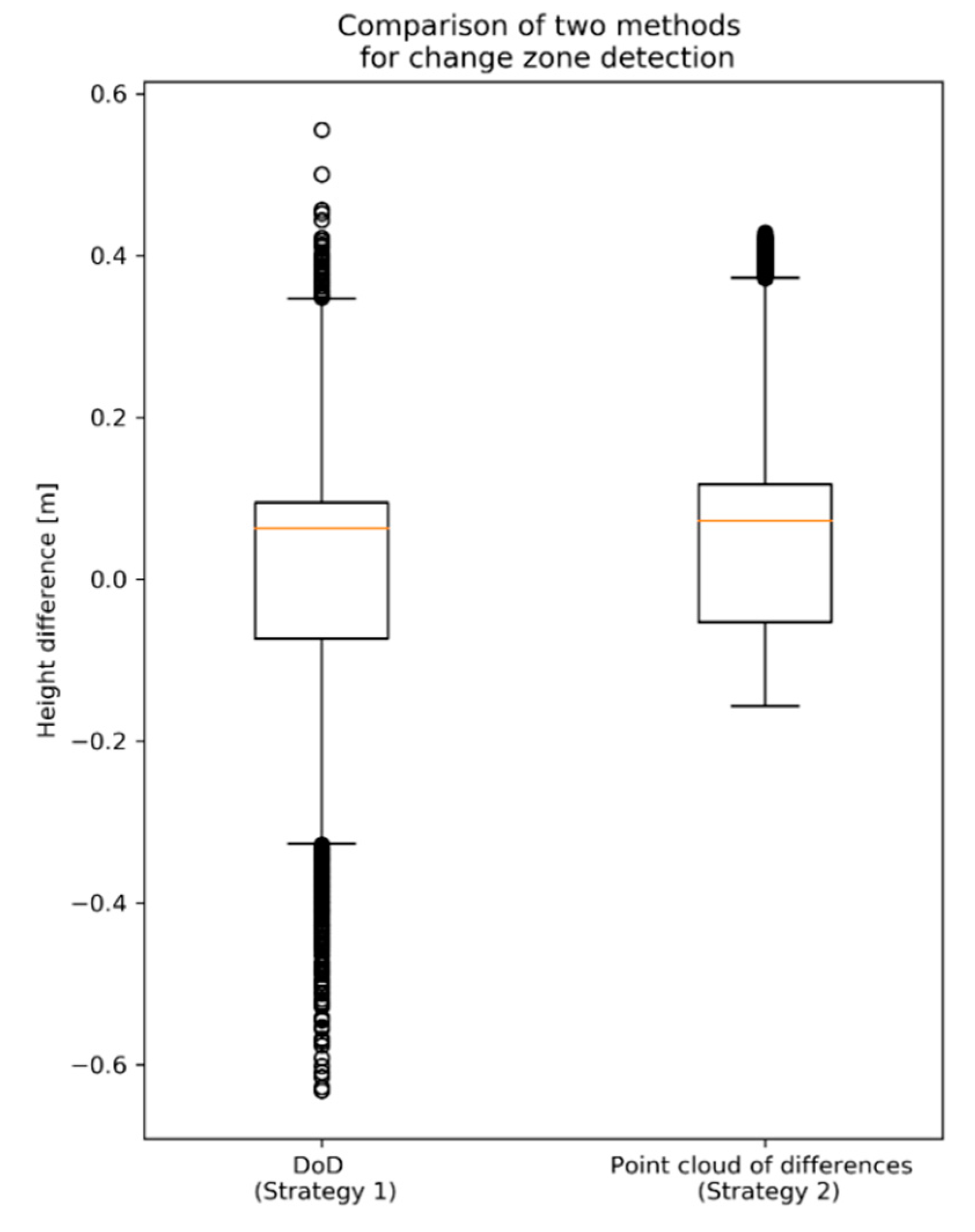
A sample area is shown in Figure 7. The area for which no points were collected is marked in black. The blue and red colors indicate the change zones with positive and negative height differences, respectively. The example of an incorrectly marked area as a change zone is highlighted in yellow, but many other mistakes can also be observed. This effect can also be noticed in the boxplot of height differences for Strategy 1 (Figure 8). Both strategies led to a similar median and upper and lower quartile of height differences. However, in contrast to Strategy 2, the application of Strategy 1 led to many outliers, representing both positive and negative height differences. These outliers resulted from interpolation errors that occurred during DEM calculation.
Due to the fact that the areas of the wrongly detected displacements were noticeably smaller for Strategy 2 (Figure 7b), differential point clouds were used to detect the change zones. Moreover, point clouds are a direct product of laser scanning measurement. Thus, point clouds are a little more accurate. Further processing of point clouds to obtain DEM leads to the generation of additional errors connected with interpolation.
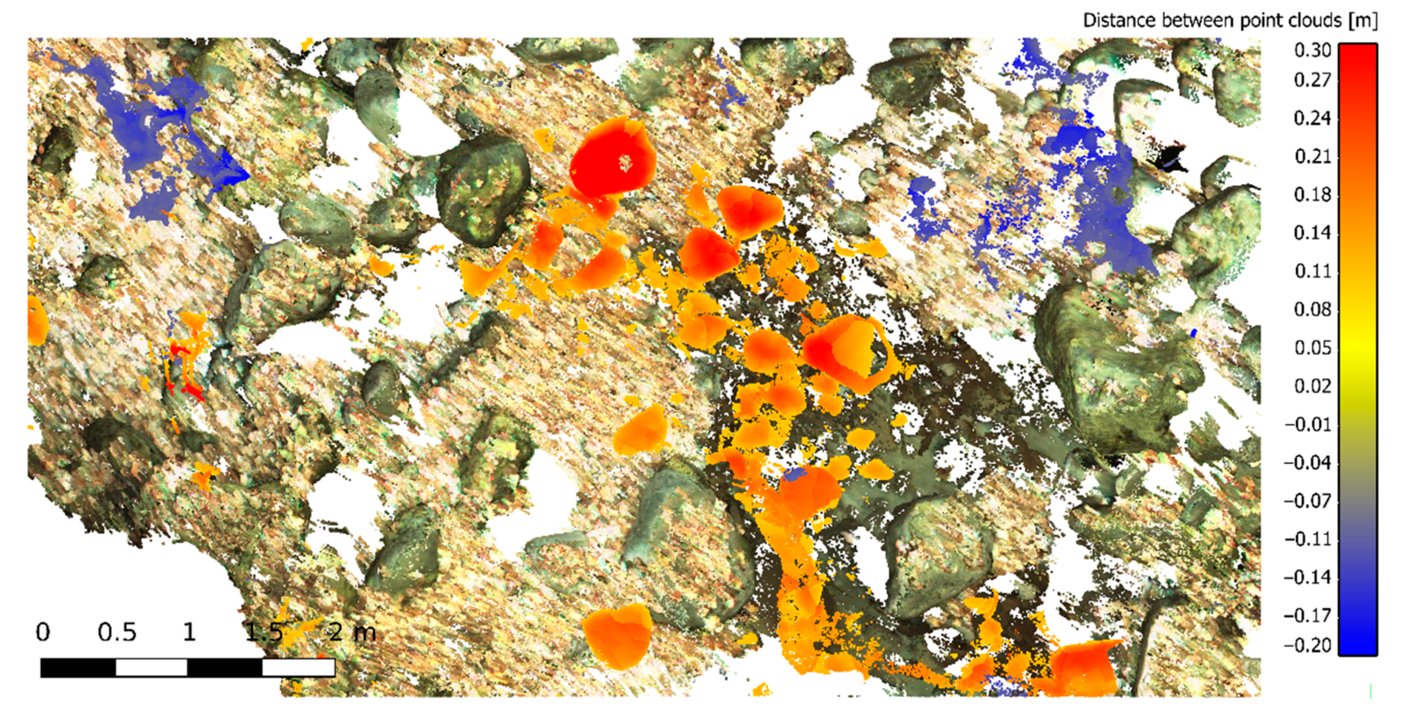
The point clouds of differences were calculated using data registered in 2011–2012, 2012–2013 (Figure 9), 2013–2014, 2014–2015, and 2015–2016 to cover the entire study period. A point cloud of difference was also created between the last and first scanning campaign (2016–2011). The 2016–2011 difference cloud spanned the entire study period. The resulting clouds indicate that bed sediment was in motion. The intensity of this movement varied during the study period.
3.2.2. 3D Displacement Determination
A visual analysis of the differential point clouds showed that it is possible to determine 3D displacement vectors between corresponding stones in different years by means of the terrestrial laser scanning technique. Examples of different types of movement are shown in Figure 10. During the analysis, it was also possible to detect single stones that were present in one year but disappeared in another and vice versa. Here, disappearance indicates that the stone was outside of the monitored area. In example A (Figure 10a), the particle with the longest axis of 600 mm was only rotated but not translated during 2012–2013. It reached a stable position in 2013 and was not moved in any of the following years. In B, another stone that has the longest axis of 750 mm was both rotated and translated, first in 2012–2013 and then in 2013–2014. In example C, the particle was not present in 2011–2013. It appeared in 2014 and remained stable.
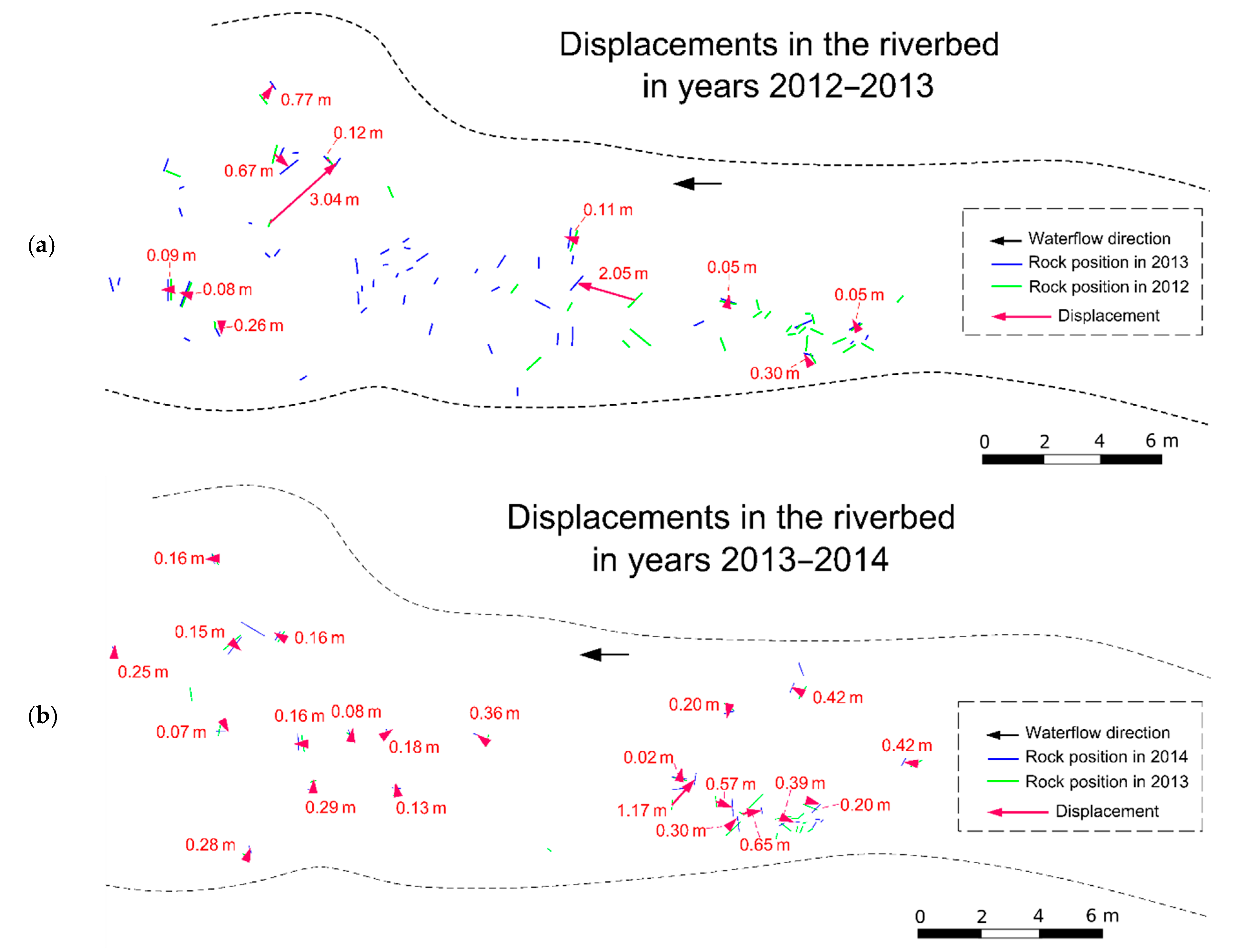
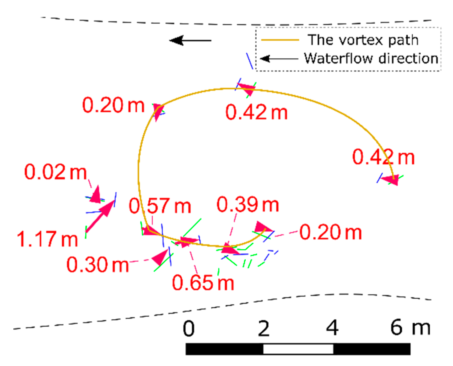
All detected movements are shown in Figure 11. The main direction of most of the displacement vectors is consistent with the water flow direction, but in some cases transverse movement also occurred, perhaps as a water vortex effect in the local riverbed pool. However, this cannot be confirmed without direct hydrological observations. This effect can also be observed for 2013–2014, where the circular movement is obvious (Figure 12). The most intense movement appeared in 2012–2013 (Figure 11a). Many particles, including boulders, were transported a long distance. The largest distance was recorded for a 320-mm diameter particle and the movement vector was oriented transversely to the water flow direction. The largest rock elements identified to have changed their position during this period had the longest axis of 800 mm and were moved for a distance of about 2 m. Many stones were brought by the water from outside of the investigation area. Taking into account the water flow direction and the position of these particles, their translation vector had to be longer than 15 m. Similar cases occurred when stones were moved outside of the area. Position changes of numerous particles also occurred during the period 2013–2014, but the movement distance was generally smaller than in the previous year. During other years, only a few stones were moved by the water. Using this method, accumulation and erosion zones may also be detected, but in most cases, individual stones remained in the same accumulation region, even when they were shifted. Similarly, it is possible to indicate compact areas both where the stones from outside of the area settled and when they were moved out.
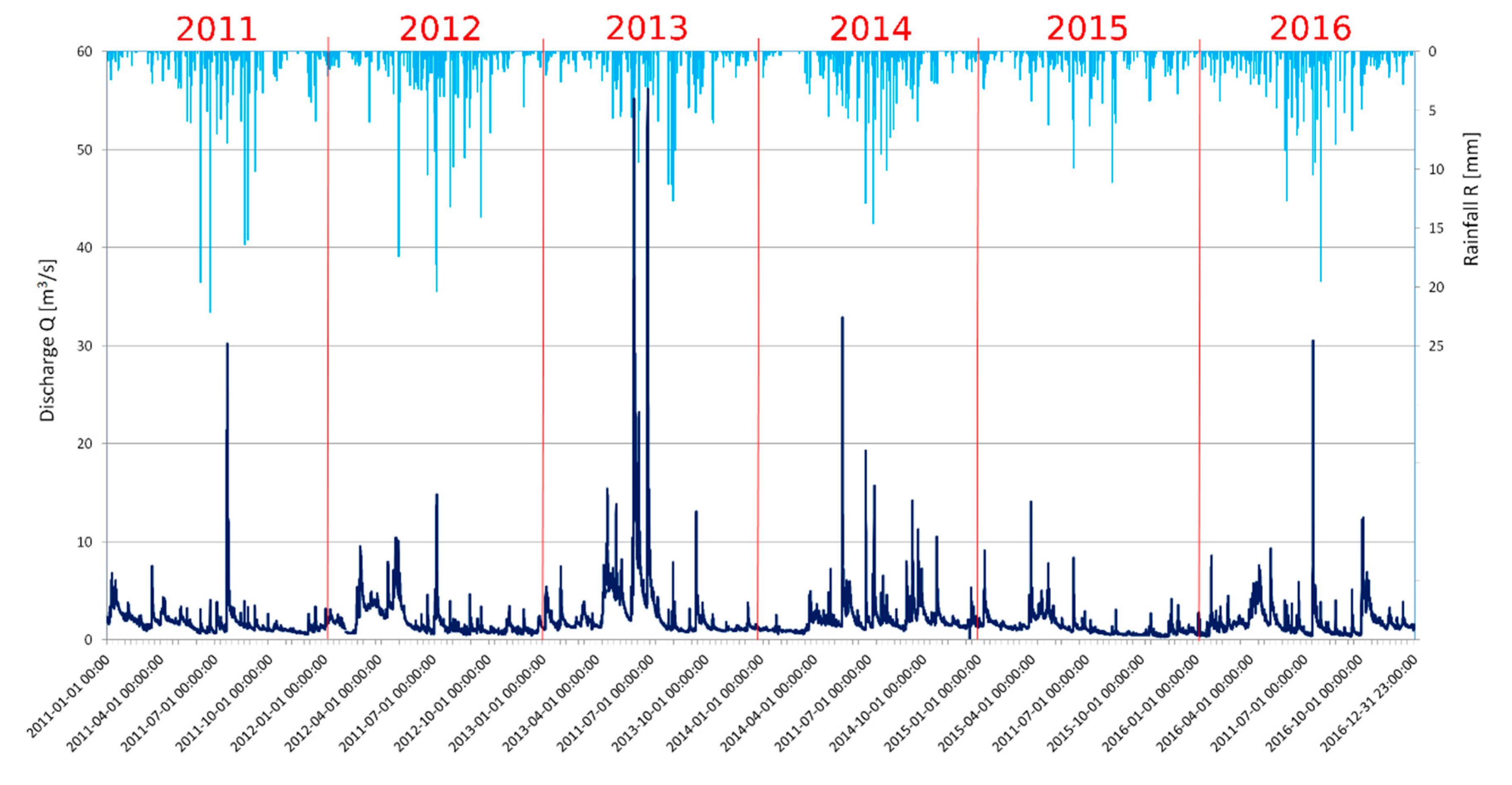
The results of the TLS measurements correspond well with the hydrological observations carried out on Łomnica (Figure 13), which may also be related to the water levels and flows of Łomniczka River. The measurements from the period of 2012–2013, when the largest displacement of coarse rock material in the riverbed was observed, include the largest spate during the observation period, at almost double the value of other years. According to the literature [35,36,37], in arctic and mountain environments, bed load transport events are caused by rainfall, snow melt, or ablation of the glacier. In the case of the Łomnica River, only the two first factors could affect the discharge rate and, consequently, bed load transport. However, it should be highlighted that in 2011–2016 there were no extreme flood events that could transport the rock material on a bigger scale. Moreover, riverbed topography is an important aspect in the determination of flow‒riverbed relationships in rivers. The topography of the riverbed is defined as the sum of the mean residual riverbed roughness and the mean riverbed slope [38]. The bed roughness is used in morphological models for the calculation of the bed shear stress and, consequently, the sediment transport rate [39]. However, the analysis described in this manuscript concerns changes in fluvial transport occurring in the same river but at different times. Therefore, the influence of riverbed roughness can be omitted in this analysis.
To the authors’ knowledge, there are only two papers ([25,26]) in which the determination of 3D vectors of particle movement is mentioned. In comparison to [26], we were able to detect more displacements and boulders were transported over longer distances, especially during 2012–2013. It was also possible to state the main direction of particle movement in 2012–2013. However, it is hard to compare the results because the river studied in this paper is different to the river investigated in [26]. In contrast to [25], in which the standard DoD method of change detection was used, in this paper, the change zones were detected by calculating the distance between the point clouds. This enabled a reduction in the number of areas falsely indicating the vertical change. Moreover, in this study, the measurement period was significantly longer than in both of those papers. Therefore, it was possible to provide a long-term analysis of changes in the riverbed, including recognition of the hydrological event (flood) responsible for the most significant morphological changes based on data available from the gauging station.
3.2.3. Limitations of the Methodology
The proposed methodology includes two steps. First, the change zones are detected. In this step, the most important factor that can influence the results is point cloud absolute accuracy. The absolute accuracy of point cloud is dependent on two factors: the accuracy of the scanner and the georeferencing accuracy. Since the accuracy of the scanner is a few millimeters (Table 2), the accuracy of measuring warp points should not be much worse. A low absolute accuracy of the point cloud may lead to improper identification of change zones, and, as a result, some of the displaced stones might be omitted. In this study, the georeferencing accuracy was about 1 cm, meaning that vertical changes over 1–2 cm (in absolute terms) can be detected. In the second step, point clouds were analyzed and the corresponding particles were found. The correspondence was found based, among other factors, on the geometry of the particles. This means that the particle can be recognized when its characteristic geometric features are visible in the point cloud. Several aspects can have an impact on the visibility of the geometric features, including the density of the point cloud and the accuracy of the laser scanner. Obviously, the TLS point cloud has a lower density for objects that are farther form the scanning position; thus, more than one scanning position should be settled. In our investigation, the average distance between the points in the areas observed from both scanner positions was about 2 mm. Despite the high point density and accuracy of the equipment used, the minimum diameter of the particle that can be manually recognized was arbitrarily designated as 10 cm. In some circumstances, e.g., an atypical shape of the particle, even smaller particles could be identified. The limitation in this step is human perception. It seems that automatic methods may identify the same rock of a smaller diameter than 10 cm; however, this can be proven or denied after the development of an automatic method. The accuracy of the point cloud also influences the displacement length. The experiments conducted in this research on the synthetic dataset showed that the displacement length was affected by a 4-cm error (Section 3.1). This means that the displacement with a length smaller than 4 cm may have been caused by point cloud inaccuracy and by the inaccurate identification of corresponding points belonging to particles in different measurement epochs. In the point cloud, there could also have been visible large shadowing effects, especially when the terrain conditions only enabled us to establish a small number of scanner stations. This may lead to the incorrect identification of corresponding particles.
3.2.4. Alternatives to TLS
The primary data used in this work are the point clouds collected with a terrestrial laser scanner; however, point clouds created from images by dense image matching [40] are of more interest and can potentially be used as an alternative data source. Usually, point clouds created from images are denser (and thus are often named as dense point clouds), but have a lower accuracy than TLS point clouds. The use of a point cloud of a higher density in the method described above may make the identification of the same stone easier, but the poor accuracy of the point cloud may lead to incorrect determination of the change zones and thus improper identification of the same stone, especially for smaller boulders or cobbles, and larger errors of determined displacement for correctly identified stones. It is very difficult to properly predict the accuracy of a dense point cloud since it depends on many factors, including object texture and illumination. However, in some circumstances, the accuracy of a dense point cloud can be very high and may be comparable to TLS point cloud accuracy. Three conditions seem to be the most important: a high accuracy of GCPs, a good quality of the sensor, and appropriate image acquisition. An indirect georeferencing method using GCPs is necessary because the accuracy of direct georeferencing is lower than the required accuracy. Note that direct georeferencing is typically performed using navigational sensors, e.g., a global navigation satellite system (GNSS) receiver and inertial measurement unit (IMU). The coordinates of GCPs should be determined with similar or better accuracy than the coordinates of TLS warp points (~1 cm); thus, a land surveying technique, i.e., total station measurements, can be used. A good-quality sensor usually means low distortion of the lens; the stability of geometrical parameters is more important, since sensor calibration can be performed and distortion can be determined. The collected images should have a high ground resolution, since, for nonphotogrammetric cameras, it is difficult to achieve better accuracy than the terrain size of one pixel (ground sampling distance—GSD). This means that images should not be taken from a larger distance, especially using short focal length lenses that benefit from a wide field of view. The distance of a few meters should allow for the achievement of GSD on the millimeter level—for an image taken from 10 m using a full-frame 36 Mpix camera equipped with a 24-mm lens, GSD is equal to about 1 mm. In addition to high resolution, high image overlap is required in order to eliminate occlusions and reduce adjustment errors. An overlap of at least 80% is typically recommended.
Appropriate images can be taken either by a human or by an unmanned aerial vehicle (UAV). The use of a UAV allows for faster acquisition, but in some circumstances it may be impossible to collect appropriate images. The first is insufficient image overlap caused by changes in UAV speed or position with respect to flight plan. This may occur when manual flight is performed, wind is pushing the UAV outside of the planned path, the accuracy of onboard navigational sensors or GNSS is low, the GNSS signal is degraded, etc. Note that small changes in speed or position cause bigger changes in overlap for a lower altitude. The second, very often overlooked, issue is the depth of field that is shorter for a shorter distance to the object. In contrast to images taken by humans, with automatic UAV flights it is impossible to control whether the object is inside the depth of field and the image is sharp. Note that autofocus cannot be used in either of the two mentioned acquisition methods since it changes the geometry for each image. The unique geometry of each image cannot be accurately determined during image block bundle adjustment.
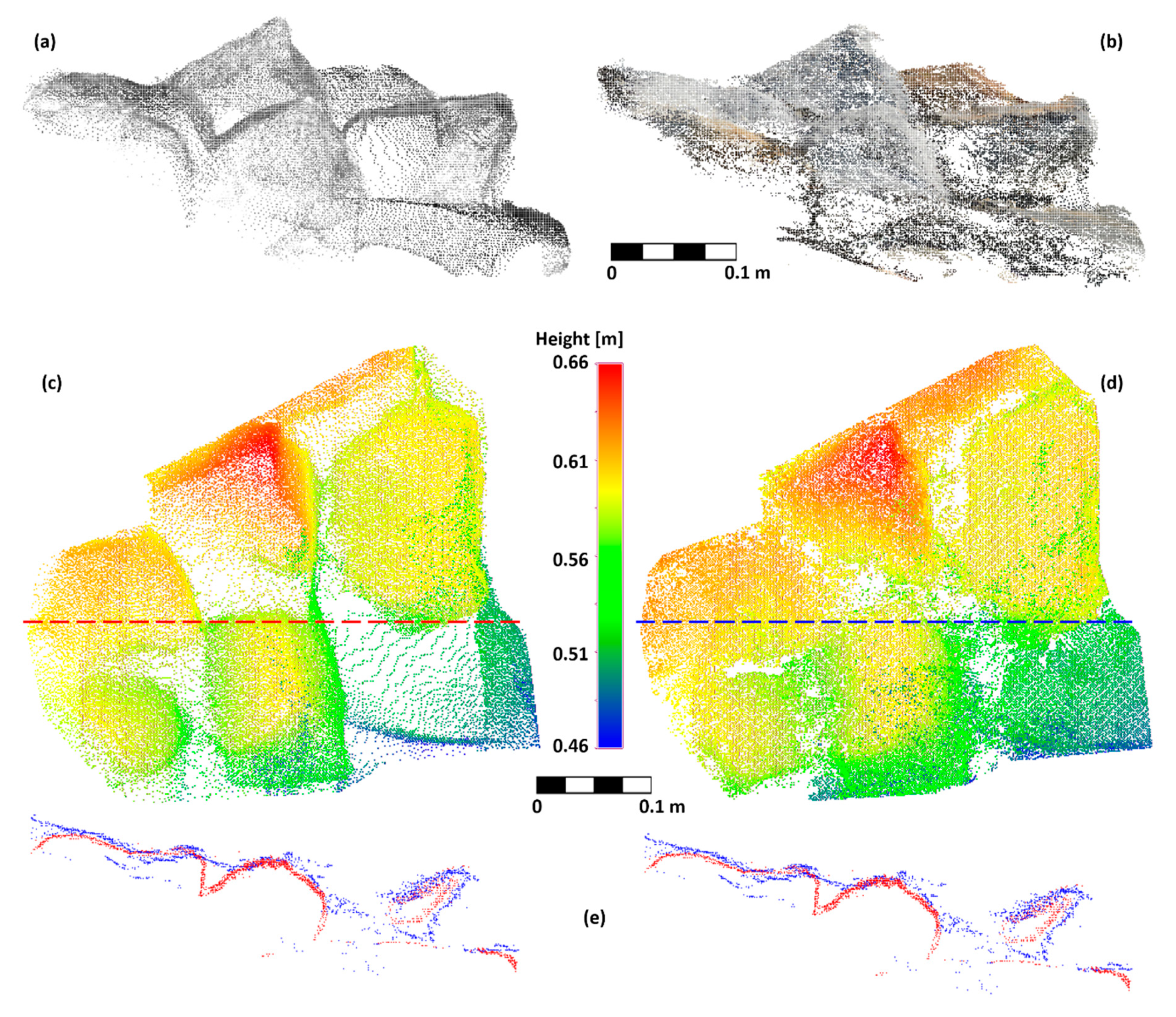
The photogrammetric data collected by humans for the synthetic test site meet the abovementioned requirements regarding the accuracy of GCPs, camera quality, size of GSD, and image overlap. This indicates that it is possible to analyze a created dense point cloud, used as an alternative to a TLS point cloud. The analysis was executed in comparison to the TLS point cloud collected for the synthetic test site. Figure 14 shows both types of point clouds for part of the scene containing a few stones.
A visual analysis of the created point clouds shows that the TLS point cloud was sparser than the dense point cloud, especially for areas between stones. This can be explained by occlusions causing these areas to be scanned only from a single scanner position, while the tops of stones were visible from all scanner positions. However, the quality of the TLS point cloud is much better than the quality of the dense point cloud. The dense point cloud contained a lot of noise points: below (inside) stones, between stones, or even above them. This was likely caused by a combination of several factors, e.g., residual errors of the bundle adjustment process, imperfection of the dense image matching process, especially during depth map creation for the “salt and pepper” texture of stones and filtering of the raw depth map. The development of dense image matching algorithms may improve the quality of the point cloud; however, some errors cannot be removed since they are object- and equipment-related. Some noise points that are outliers (e.g., lying below stones) can be removed by applying point cloud filtering algorithms [41], but others (e.g., points between stones that fill the gap) stay since they are not outliers. This type of noise point may cause two stones to be visible as a single stone, but it may happen that only one stone can be moved. Consequently, the displacement of such a stone cannot be determined using the method described in this paper.
A worse quality of the dense point cloud than the TLS point cloud is less relevant if it is used to create subsequent photogrammetric products, such as an orthomosaic. Note that reference measurements in the synthetic test field were executed manually on the high-resolution orthomosaic (GSD = 1 mm). However, for an automatic algorithm that detects the same stone based on point clouds, it would be more efficient to use point clouds of a better quality. This justifies the use of TLS technology in our study. In the future, images can be considered as a source of 3D data, since more robust image processing algorithms are still being developed.
4. Conclusions
The monitoring of bed load transport is essential for many environmental applications. This issue can be studied using traditional methods, such as tracers or sediment traps, but nowadays TLS is becoming increasingly popular in this research field.
In this study, the problem of fluvial transport of river bed coarse grain particles was investigated by means of terrestrial laser scanning. The study covered a period of six years of fluvial transport monitoring in a steeply inclined mountain river environment characterized by an extremely complex spatial distribution of particles.
To date, the need to determine the displacement vectors for individual particles in the riverbed has only been postulated in the literature. We assessed these displacements for the real-world conditions of a mountain river. Unlike many other publications, in our study, we analyzed a long time series of TLS data.
Two strategies were tested to detect the change zones. The first strategy was based on differential DEM creation; the second involved the calculation of differences between point clouds instead of DEMs. The experiments showed that the second strategy was more beneficial. Based on the detected areas of change, the movement of the boulders was traced and the displacements of the stones were determined.
Most of the changes appeared in 2012–2013 and 2013–2014. The most intense movement appeared in 2012–2013, when many particles, including boulders, were shifted long distances. In this period, numerous stones were moved outside of the investigation area. Under the observed hydrological conditions, particles with diameters greater than 0.8 m were not the subject of any movement. The movement of boulders with diameters of about 0.5 m was also rare. The main direction of most of the displacement vectors was consistent with the water flow direction, but in some cases transverse movement occurred. As a result, it can be stated that, in the observed hydrological conditions, the riverbed of Łomniczka River remained stable and the morphology and riverbed pavement were capable of conducting much greater water flows.
The methodology of point cloud analysis applied in this investigation allowed us to automatically detect change zones and even individual particles that changed their position. Moreover, the manual analysis of the point cloud allowed us to recognize different types of movement and to calculate the 3D movement distance of individual particles with an accuracy of 4 cm. The minimal diameter of the particle that can be manually recognized was arbitrarily designated as about 10 cm.
However, there is a need to develop an automatic method for the calculation of the movement parameters of individual coarse grain particles. Automatic tracking of particle movement is extremely challenging. Matching corresponding particles to different point clouds may be impossible because the movement of the stone can include not only translation but also rotation components in 3D space. As a result, in the two compared measurement epochs, different sides of the stone could be measured, which prevented us from finding geometrical matches. The development of a matching method that eliminates these shortcomings will be the subject of future work.
Author Contributions
A.W., G.J., and A.B. designed the experiment and performed the measurements. A.W. and A.B. discussed the results and wrote the paper. A.W. performed the calculations and prepared the figures. M.K. proposed the study area, provided its description, and described the hydrological conditions.
Funding
This research received no external funding.
Acknowledgments
The authors express their gratitude to the IMGW (Institute of Meteorology and Water Management, National Research Institute, Poland) for providing the hydrological and precipitation data. The LiDAR data used for this study (Figure 1) have been purchased and used with academic license DIO.DFT.DSI.7211.1619.2015_PL_N, according to the Polish law regulations in the administration of Główny Urząd Geodezji i Kartografii (Head Office of Land Surveying and Cartography).
Conflicts of Interest
The authors declare no conflict of interest.
References
- Wilcock, P.R. Toward a practical method for estimating sediment-transport rates in gravel-bed rivers. Earth Surf. Process. Landf. 2001, 26, 1395–1408. [Google Scholar] [CrossRef]
- Recking, A.; Frey, P.; Paquier, A.; Belleudy, P.; Champagne, J.Y. Feedback between bed load transport and flow resistance in gravel and cobble bed rivers. Water Resour. Res. 2008, 44, 1–21. [Google Scholar] [CrossRef]
- Garcia, C.; Laronne, J.B.; Sala, M. Continuous monitoring of bedload flux in a mountain gravel-bed river. Geomorphology 2000, 34, 23–31. [Google Scholar] [CrossRef]
- Bunte, K.; Abt, S.R.; Potyondy, J.P.; Ryan, S.E. Measurement of coarse gravel and cobble transport using portable bedload traps. J. Hydraul. Eng. 2004, 130, 879–893. [Google Scholar] [CrossRef]
- Bergman, N.; Laronne, J.B.; Reid, I. Benefits of design modifications to the Birkbeck bedload sampler illustrated by flash-floods in an ephemeral gravel-bed channel. Earth Surf. Process. Landf. 2007, 32, 317–328. [Google Scholar] [CrossRef]
- Allan, J.C.; Hart, R.; Tranquili, J.V. The use of Passive Integrated Transponder (PIT) tags to trace cobble transport in a mixed sand-and-gravel beach on the high-energy Oregon coast, USA. Mar. Geol. 2006, 232, 63–86. [Google Scholar] [CrossRef]
- Bradley, D.N.; Tucker, G.E. Measuring gravel transport and dispersion in a mountain river using passive radio tracers. Earth Surf. Process. Landf. 2012, 37, 1034–1045. [Google Scholar] [CrossRef]
- Hassan, M.A.; Voepel, H.; Schumer, R.; Parker, G.; Fraccarollo, L. Displacement characteristics of coarse fluvial bed sediment. J. Geophys. Res. Earth Surf. 2013, 118, 155–165. [Google Scholar] [CrossRef]
- Phillips, C.B.; Martin, R.; Jerolmack, D.J. Impulse framework for unsteady flows reveals superdiffusive bed load transport. Geophys. Res. Lett. 2013, 40, 1328–1333. [Google Scholar] [CrossRef] [Green Version]
- Ancey, C.; Heyman, J. A microstructural approach to bed load transport: mean behaviour and fluctuations of particle transport rates. J. Fluid Mech. 2014, 744, 129–168. [Google Scholar] [CrossRef] [Green Version]
- Olinde, L.; Johnson, J.P.L. Using RFID and accelerometer-embedded tracers to measure probabilities of bed load transport, step lengths, and rest times in a mountain stream. Water Resour. Res. 2015, 51, 7572–7589. [Google Scholar] [CrossRef] [Green Version]
- Ancey, C. Stochastic modeling in sediment dynamics: Exner equation for planar bed incipient bed load transport conditions. J. Geophys. Res. Space Phys. 2010, 115. [Google Scholar] [CrossRef]
- Recking, A.; Liébault, F.; Peteuil, C.; Jolimet, T. Testing bedload transport equations with consideration of time scales. Earth Surf. Process. Landf. 2012, 37, 774–789. [Google Scholar] [CrossRef]
- Haddadchi, A.; Omid, M.H.; Dehghani, A.A. Bedload equation analysis using bed load-material grain size. J. Hydrol. Hydromech. 2013, 61, 241–249. [Google Scholar] [CrossRef]
- Vázquez-Tarrío, D.; Menéndez-Duarte, R. Assessment of bedload equations using data obtained with tracers in two coarse-bed mountain streams (Narcea River basin, NW Spain). Geomorphol. 2015, 238, 78–93. [Google Scholar] [CrossRef]
- Vosselman, G.; Maas, H.G. Airborne and Terrestrial Laser Scanning; Whittles Publishing: Scotland, UK, 2010; pp. 1–336. [Google Scholar]
- Heritage, G.L.; Milan, D.J. Terrestrial Laser Scanning of grain roughness in a gravel-bed river. Geomorphology 2009, 113, 4–11. [Google Scholar] [CrossRef]
- Theule, J.I.; Liebault, F.; Loye, A.; Laigle, D.; Jaboyedoff, M. Sediment budget monitoring of debris-flow and bedload transport in the Manival Torrent, SE France. Nat. Hazards Earth Syst. Sci. 2012, 12, 731–749. [Google Scholar] [CrossRef] [Green Version]
- Picco, L.; Mao, L.; Cavalli, M.; Buzzi, E.; Rainato, R.; Lenzi, M. Evaluating short-term morphological changes in a gravel-bed braided river using terrestrial laser scanner. Geomorphology 2013, 201, 323–334. [Google Scholar] [CrossRef]
- Kuo, C.-W.; Brierley, G.; Chang, Y.H. Monitoring channel responses to flood events of low to moderate magnitudes in a bedrock-dominated river using morphological budgeting by terrestrial laser scanning. Geomorphology 2015, 235, 1–14. [Google Scholar] [CrossRef]
- Brasington, J.; Vericat, D.; Rychkov, I. Modeling river bed morphology, roughness, and surface sedimentology using high resolution terrestrial laser scanning. Water Resour. Res. 2012, 48, W11519. [Google Scholar] [CrossRef]
- Baewert, H.; Bimböse, M.; Bryk, A.; Rascher, E.; Schmidt, K.-H.; Morche, D. Roughness determination of coarse grained alpine river bed surfaces using Terrestrial Laser Scanning data. Z. Geomorphol. Suppl. Issues 2014, 58, 81–95. [Google Scholar] [CrossRef]
- Hodge, R.; Brasington, J.; Richards, K. Analysing laser-scanned digital terrain models of gravel bed surfaces: linking morphology to sediment transport processes and hydraulics. Sedimentology 2009, 56, 2024–2043. [Google Scholar] [CrossRef]
- Williams, R.; Rennie, C.; Brasington, J.; Hicks, M.; Vericat, D. Linking the spatial distribution of bed load transport to morphological change during high-flow events in a shallow braided river. J. Geophys. Res. 2013, 120, 604–622. [Google Scholar] [CrossRef]
- Jozkow, G.; Borkowski, A.; Kasprzak, M. Monitoring of fluvial transport in the mountain river bed using terrestrial laser scanning. ISPRS Int. Arch. Photogramm. Remote Sens. Spat. Inf. Sci. 2016, 41, 523–528. [Google Scholar] [CrossRef]
- Lotsari, E.; Wang, Y.; Kaartinen, H.; Jaakkola, A.; Kukko, A.; Vaaja, M.; Hyyppä, H.; Hyyppä, J.; Alho, P. Gravel transport by ice in a subarctic river from accurate laser scanning. Geomorphology 2015, 246, 113–122. [Google Scholar] [CrossRef]
- Dubicki, A.; Mordalska, H.; Tokarczyk, T.; Adynkiewicz-Piragas, M. Wody Powierzchniowe Karkonoszy (Surface Water of Karkonosze Mountains). In Karkonosze: Przyroda nieożywiona i człowiek (Karkonosze: Inanimate Nature and Man); Mierzejewski, M.P., Ed.; Wyd. Uniwersytetu Wrocławskiego: Wrocław, Poland, 2005; pp. 399–425. (In Polish) [Google Scholar]
- Bieroński, J.; Pawlak, W.; Tomaszewski, J. Komentarz do Mapy Hydrograficznej w Skali 1:50 000 (Comment on the Hydrographical Map in Scale 1:50000); Arkusz (sheet) M-33-44-C Szklarska Poręba; GEPOL: Poznań, Poland, 2002. (In Polish) [Google Scholar]
- Kasprzak, M.; Migoń, P. Historical and recent floods in the West Sudetes—geomorphological dimension. Z. Geomorphol. Suppl. Issues 2015, 59, 73–97. [Google Scholar] [CrossRef]
- Smith, M.; Vericat, D.; Gibbins, C. Through-water terrestrial laser scanning of gravel beds at the patch scale. Earth Surf. Process. Landforms. 2012, 37, 411–421. [Google Scholar] [CrossRef]
- Heritage, G.; Hetherington, D. Towards a protocol for laser scanning in fluvial Geomorphology. Earth Surf. Process. Landf. 2007, 32, 66–74. [Google Scholar] [CrossRef]
- Wang, Y.; Liang, X.; Flener, C.; Kukko, A.; Kaartinen, H.; Kurkela, M.; Vaaja, M.; Hyyppä, H.; Alho, P. 3D Modeling of Coarse Fluvial Sediments Based on Mobile Laser Scanning Data. Remote Sens. 2013, 5, 4571–4592. [Google Scholar] [CrossRef] [Green Version]
- Bangen, S.G.; Wheaton, J.M.; Bouwes, N.; Bouwes, B.; Jordan, C. A methodological intercomparison of topographic survey techniques for characterizing wadeable streams and rivers. Geomorphology 2014, 206, 343–361. [Google Scholar] [CrossRef]
- Girardeau-Montaut, D. CloudCompare—Open Source Project. 2016. Available online: http://www.danielgm.net/cc/ (accessed on 26 April 2017).
- Lana-Renault, N.; Alvera, B.; García-Ruiz, J.M. Runoff and sediment transport during the snowmelt period in a Mediterranean high-mountain catchment. Arct. Antarct. Alp. Res. 2011, 43, 213–222. [Google Scholar] [CrossRef]
- Beylich, A.A.; Gintz, D. Effects of high-magnitude/low-frequency fluvial events generated by intense snowmelt or heavy rainfall in arctic periglacial environments in northern Swedish Lapland and Northern Siberia. Geogr. Ann. Ser. A Phys. Geogr. 2004, 86, 11–29. [Google Scholar] [CrossRef]
- Kociuba, W.; Janicki, G.; Siwek, K.; Gluza, A. Bedload transport as an indicator of contemporary transformations of arctic fluvial systems. DEBRIS Flows 2012, 1, 125–135. [Google Scholar]
- Noss, C.; Lorke, A. Roughness, resistance, and dispersion: Relationships in small streams. Water Resour. Res. 2016, 52, 2802–2821. [Google Scholar] [CrossRef] [Green Version]
- Tuijnder, A.P.; Ribberink, J.S. Experimental observation and modelling of roughness variation due to supply-limited sediment transport in uni-directional flow. J. Hydraul. Res. 2012, 50, 506–520. [Google Scholar] [CrossRef]
- Remondino, F.; Spera, M.G.; Nocerino, E.; Menna, F.; Nex, F. State of the art in high density image matching. Photogramm. Rec. 2014, 29, 144–166. [Google Scholar] [CrossRef] [Green Version]
- Wolff, K.; Kim, C.; Zimmer, H.; Schroers, C.; Botsch, M.; Sorkine-Hornung, O.; Sorkine-Hornung, A. Point Cloud Noise and Outlier Removal for Image-Based 3D Reconstruction. In Proceedings of the 2016 4th International Conference on 3D Vision (3DV), Stanford, CA, USA, 25–28 October 2016; pp. 118–127. [Google Scholar]
Figure 1.
Test site location (a) and upper part of the investigated section of the Łomniczka riverbed (b).
Figure 1.
Test site location (a) and upper part of the investigated section of the Łomniczka riverbed (b).

Figure 2.
Scanning geometry on the study area.

Figure 3.
Shadowing effects (large white areas) in terrestrial laser scanning (TLS) point cloud.

Figure 4.
Flowchart of two tested strategies of 3D movement determination. In Strategy 1 (left), the identification of change zones was performed using DEM of difference (DoD). In Strategy 2 (right), the identification of change zones was performed using cloud-to-cloud distance.
Figure 4.
Flowchart of two tested strategies of 3D movement determination. In Strategy 1 (left), the identification of change zones was performed using DEM of difference (DoD). In Strategy 2 (right), the identification of change zones was performed using cloud-to-cloud distance.

Figure 5.
Validation dataset—orthomosaic created for the first epoch (before particle displacement). The white squares with black marks are the GCP targets. The enlargement shows one of the particles marked with a number. Marked particles were later displaced.
Figure 5.
Validation dataset—orthomosaic created for the first epoch (before particle displacement). The white squares with black marks are the GCP targets. The enlargement shows one of the particles marked with a number. Marked particles were later displaced.

Figure 6.
Displacements between two scanning epochs in the simulated dataset.

Figure 7.
Change zones (blue and red areas) detected using Strategy 1 (a) and Strategy 2 (b). The yellow circle highlights the example of incorrectly identified change.
Figure 7.
Change zones (blue and red areas) detected using Strategy 1 (a) and Strategy 2 (b). The yellow circle highlights the example of incorrectly identified change.

Figure 8.
Box plots representing the distribution of height differences indicating change zones in both strategies.
Figure 8.
Box plots representing the distribution of height differences indicating change zones in both strategies.

Figure 9.
Part of the point cloud from 2012, with significant height differences between 2012 and 2013. Positive height differences are in orange‒red and negative height differences are in violet‒blue.
Figure 9.
Part of the point cloud from 2012, with significant height differences between 2012 and 2013. Positive height differences are in orange‒red and negative height differences are in violet‒blue.

Figure 10.
Examples of particles movement. (a) Green—position of stone A in 2012, red—position of stone A in 2013; (b) green—position of stone B in 2012, red—position of stone B in 2013, yellow—position of stone B in 2014, pink—position of stone C in 2014.
Figure 10.
Examples of particles movement. (a) Green—position of stone A in 2012, red—position of stone A in 2013; (b) green—position of stone B in 2012, red—position of stone B in 2013, yellow—position of stone B in 2014, pink—position of stone C in 2014.

Figure 11.
Displacements in the riverbed in different years. Displacements smaller than 0.5 m are indicated with an arrowhead only.
Figure 11.
Displacements in the riverbed in different years. Displacements smaller than 0.5 m are indicated with an arrowhead only.

Figure 12.
Example of the probable vortex effect.

Figure 13.
Hourly discharge (dark blue line) for the Łomnica River gauging station and hourly precipitation (light blue lines) for the Karpacz meteorological station in 2011–2016. Data source: Institute of Meteorology and Water Management, National Research Institute.
Figure 13.
Hourly discharge (dark blue line) for the Łomnica River gauging station and hourly precipitation (light blue lines) for the Karpacz meteorological station in 2011–2016. Data source: Institute of Meteorology and Water Management, National Research Institute.

Figure 14.
Point clouds and cross sections for several stones of the synthetic test field. First row: XZ projection of (a) TLS point cloud colored by intensity values, (b) dense point cloud colored by RGB values. Second row: XY projection of: (c) TLS point cloud, (d) dense point cloud; the colors show the Z coordinates and the red and blue lines show the location of 5-mm-thick cross sections through the dense and TLS point clouds, respectively. (e) Cross-sectional points of the TLS point cloud (in red) and the dense point cloud (in blue). The image showing cross sections was repeated for both columns for correspondence with both point clouds.


Table 1.
Hydrological statistics of the Łomniczka River [27].
Table 1.
Hydrological statistics of the Łomniczka River [27].
| Watercourse Characteristics | Upper Gauge Station | Lower Gauge Station (Karpacz) |
|---|---|---|
| Length of the stream | 0.55 km | 6.5 km |
| Catchment area | 0.46 km2 | 12.1 km2 |
| Average inclination of the stream | 89‰ | 136‰ |
| Average annual low water level | – | 111 cm |
| Average annual medium water level | – | 121 cm |
| Average annual high water level | – | 169 cm |
| Average annual low flow | 0.007 m3 s−1 | 0.09 m3 s−1 |
| Average annual medium flow | 0.024 m3 s−1 | 0.42 m3 s−1 |
| Average annual high flow | 0.71 m3 s−1 | 9.09 m3 s−1 |
| Maximum recorded water level | – | 260 cm (7 July 1997) |
| Maximum recorded water flow | – | 51.6 m3 s−1 (7 July 1997) |
Table 2.
Selected parameters of Leica ScanStation C10 and Leica ScanStation P20.
| Parameter | Leica ScanStation C10 | Leica ScanStation P20 |
|---|---|---|
| Laser wavelength | 532 nm (green) | 808 nm/658 nm (infrared/red) |
| Horizontal field of view | 360° | 360° |
| Vertical field of view | 270° | 270° |
| Range | 300 m @90% albedo | 120 m |
| 134 m @18% albedo | ||
| Maximum scan rate | 50,000 points/s | 1,000,000 points/s |
| Point 3D position accuracy | 6 mm | 3 mm |
| Range accuracy | 4 mm | <1 mm |
| Target acquisition standard deviation | 2 mm | 2 mm |
Table 3.
Registration and georeferencing accuracy.
| Measurement Epoch | 2011 | 2012 | 2013 | 2014 | 2015 | 2016 |
|---|---|---|---|---|---|---|
| Date of measurement | 10 November | 23 October | 24 October | 4 October | 30 October | 17 November |
| Registration mean absolute error (mm) | 1 | 1 | 2 | 2 | 2 | 2 |
| Georeferencing mean absolute error (mm) | 3 | 11 | 6 | 4 | 5 | 8 |
Table 4.
Number of correctly and incorrectly identified types of movement.
| Movement Type | Correctly Identified | Incorrectly Identified | Not Identified |
|---|---|---|---|
| Moved particles | 14 | 1 | 0 |
| New particles in the area | 3 | 0 | 0 |
| Particles removed from the area | 0 | 0 | 1 |
Table 5.
Displacement values from point clouds (D) and reference values (DRef) from the orthomosaic.
Table 5.
Displacement values from point clouds (D) and reference values (DRef) from the orthomosaic.
| Number | Distance (D) (m) | Reference Distance (DRef) (m) | ∆D = D − DRef (m) |
|---|---|---|---|
| 1 | 0.12 | 0.12 | 0 |
| 2 | 0.11 | 0.11 | 0 |
| 3 | 0.89 | 0.90 | 0.01 |
| 4 | 0.30 | 0.30 | 0 |
| 5 | 0.41 | 0.40 | 0.01 |
| 6 | 1.27 | 1.26 | 0.01 |
| 7 | 0.15 | 0.06 | 0.09 |
| 8 | 0.85 | 0.82 | 0.03 |
| 9 | 0.03 | 0.05 | −0.02 |
| 10 | 1.58 | 1.60 | −0.02 |
| 11 | 1.13 | 1.16 | −0.03 |
| 12 | 0.58 | 0.58 | 0 |
| 13 | 1.02 | 1.13 | −0.11 |
| 14 | 0.22 | 0.21 | 0.01 |
| RMSE | 0.04 | ||
© 2019 by the authors. Licensee MDPI, Basel, Switzerland. This article is an open access article distributed under the terms and conditions of the Creative Commons Attribution (CC BY) license (http://creativecommons.org/licenses/by/4.0/).
Share and Cite
MDPI and ACS Style
Walicka, A.; Jóźków, G.; Kasprzak, M.; Borkowski, A. Terrestrial Laser Scanning for the Detection of Coarse Grain Size Movement in a Mountain Riverbed. Water 2019, 11, 2199. https://doi.org/10.3390/w11112199
AMA Style
Walicka A, Jóźków G, Kasprzak M, Borkowski A. Terrestrial Laser Scanning for the Detection of Coarse Grain Size Movement in a Mountain Riverbed. Water. 2019; 11(11):2199. https://doi.org/10.3390/w11112199
Chicago/Turabian StyleWalicka, Agata, Grzegorz Jóźków, Marek Kasprzak, and Andrzej Borkowski. 2019. "Terrestrial Laser Scanning for the Detection of Coarse Grain Size Movement in a Mountain Riverbed" Water 11, no. 11: 2199. https://doi.org/10.3390/w11112199
Note that from the first issue of 2016, this journal uses article numbers instead of page numbers. See further details here.