


ABSTRACT
We report the experimental set-up and overall results of the AARTFAAC wide-field radio survey, which consists of observing the sky within 50° of Zenith, with a bandwidth of 3.2 MHz, at a cadence of 1 s, for 545 h. This yielded nearly 4 million snapshots, two per second, of on average 4800 square degrees and a sensitivity of around 60 Jy. We find two populations of transient events, one originating from PSR B0950+08 and one from strong ionospheric lensing events, as well as a single strong candidate for an extragalactic transient, with a peak flux density of 80 ± 30 Jy and a dispersion measure of |$73\pm 3\, \mathrm{~pc~cm^{-3}}$|. We also set a strong upper limit of 1.1 all-sky per day to the rate of any other populations of fast, bright transients. Lastly, we constrain some previously detected types of transient sources by comparing our detections and limits with other low-frequency radio transient surveys.
1 INTRODUCTION
Discoveries of astronomical transients not infrequently occur by chance, during observations designed for other purposes, e.g. in case solar-flare gamma-ray outbursts (Peterson & Winckler 1959), radio pulsars (Hewish et al. 1968), and gamma-ray bursts (GRBs) (Klebesadel, Strong & Olson 1973). Some, however, are the result of deliberately designed surveys, either to explore a new part of parameter space (e.g. Stewart et al. 2016), or to search for more examples of known type of transient, in recent history notably fast radio bursts (FRBs) (e.g. CHIME & ARTS, CHIME/FRB Collaboration 2019a; Oostrum et al. 2020). Others are set up with a specific goal, and then find or study a great wealth of other phenomena, such as the OGLE experiment (see e.g. Paczynski et al. 1996). By now of course there are many such experiments at optical wavelengths (Kaiser 2004; Rau et al. 2009; Bellm et al. 2019).
The discovery of as-of-yet unobserved phenomena in a new part of parameter space has been a key science goal of the Low-Frequency Array (LOFAR; van Haarlem et al. 2013) since its inception (Fender et al. 2006). AARTFAAC, the Amsterdam-ASTRON Radio Transient Facility and Analysis Center, is a project developed to utilize LOFAR’s central stations to expand its transients discovery space to even wider fields and faster cadences, but at relatively poor angular resolution and sensitivity: it searches for the rarest and brightest transient and variable phenomena on seconds time-scale. As a dedicated transient detector, its goal is to maximize the useful information recorded, near-real time, and generate alerts for broadcast to the multiwavelength transient community.
Beyond discovering entirely new classes of transient events, our blind survey allows us to constrain surface density-brightness limits on the low-frequency counterparts to known transient and variable sources. Even upper limits to the prompt emission from mergers of binary neutron stars or neutron-star black hole binaries could aid in determining the neutron star equation of state; for GRBs and magnetar outbursts, the host environment and emission physics could be constrained (e.g. Gaensler et al. 2005; Granot & van der Horst 2014; Burlon et al. 2015, and references therein); for FRBs the rates and/or the low-frequency spectrum and emission mechanism might be constrained (Rajwade & Lorimer 2017).
Realizing the goal of a near-real time transient detection requires the development of algorithms that calibrate and image the radio data very rapidly and then automatically filter an enormous number of spurious candidates from the large number of potential transients found in the resulting image stream. This in turn requires thorough characterization of the instrument and data. Therefore, while the primary purpose of our survey is to detect bright, low-frequency, transient events that evolve on time-scales of seconds, our secondary purpose is the development of a detection pipeline which can monitor our data stream and produce a reasonable number of candidates for closer inspection.
We performed a blind survey at 60 MHz for transient events with time-scales down to 1 s. In doing so we developed a novel method for analysing light curves to detect any potentially interesting events, while reducing detections of specious sources, e.g. noise, interference, satellites, and airplanes. With that, we observed various phenomena, from extreme-fluence pulsar outbursts (Kuiack et al. 2020), to isolated scintels magnifying persistent sources and scintillating structures lasting many hours (Kuiack et al. 2021). In this paper, we present the overall data analysis strategy of the survey and limits to the surface densities of any as yet undiscovered phenomena, and compare these results with other recent low-frequency transient surveys; we also report the discovery of a potential cosmic transient.
In Section 2, we briefly describe the instrument and data products analysed, and the set of observations gathered. Next, in Section 3 we outline the method we have developed to analyse our source data bases, and detect potentially astrophysically interesting events. Our results are presented in Section 4, followed by a discussion of our findings in the context of other recent surveys in Section 5. Lastly, we conclude ins Section 6.
2 INSTRUMENT AND OBSERVATION
2.1 Instrument
AARTFAAC is a multipurpose, wide-field, fast cadence imaging, low-frequency radio project (Prasad et al. 2014, 2016). It operates as a parallel back end, utilizing the low-band antennae (LBA) simultaneously during other regularly scheduled LOFAR observations. Since AARTFAAC can only operate during LBA observations and some otherwise unscheduled (filler) time, the observation times and duration are somewhat random, and a single observation can last from under 1 to 24 h. Signal is taken directly from 288 dipoles in the outer rings of the central six LOFAR stations, providing a maximum baseline of 300 m and yielding a spatial resolution of 1° at 60 MHz. The dipole response pattern, together with our correlating, calibration, and imaging pipeline, produces Zenith-pointing snapshots with a sensitivity to the full sky, decreasing from best at Zenith to very poor on the horizon (Prasad et al. 2014, 2016).
Complex gain calibration, for both direction-dependent and direction-independent effects, is performed in real-time using a multisource self-calibration algorithm (Wijnholds & van der Veen 2009). Calibration is done on each time-step and frequency sub-band independently; to increase throughput converged solutions from previous time-steps are used as starting points for the solution at the next time-step. The sky model used is composed of the five brightest sources in the radio sky, Cassiopeia A, Cygnus A, Taurus A, Virgo A, and the Sun. Each is modelled as a single Gaussian, an accurate enough representation given AARTFAAC resolution. In order to reveal the fainter sources the bright calibrators are then subtracted. A full detailed description of the calibration method is given by Prasad et al. (2014).
Calibrated visibilities are then streamed live to disc and to an imaging pipeline which performs an FFT on the gridded visibilities. Additionally, sensitivity to the large-scale Galactic emission is reduced by removing baselines shorter than 10λ (where λ = 5 m at 60 MHz). Lastly, a primary beam correction is applied, which flattens the antenna response across the field of view (Kuiack et al. 2018). An example of a snapshot image is given in the left-hand panel of Fig. 1. This yields a typical background noise of 7.5 Jy beam−1 at Zenith for images generated by integrating eight consecutive sub-bands. This is somewhat less than the theoretical confusion noise limit of 10.4 Jy beam−1 (equation 6; van Haarlem et al. 2013). The full pipeline introduces a total latency of around 1.5 s from the received signal to the output image.
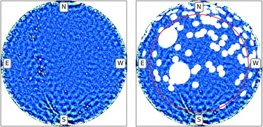
Left: An example single AARTFAAC snapshot image. Right: The remaining sky area surveyed after regions around the AARTFAAC catalogue sources and A-team have been excluded. The red circle indicates the extent of the detection region, 50° from Zenith. The outer edge of the image is at elevation 4°, in order to cut off the worst noise close to the horizon. After excluding 3° around the AARTFAAC catalogue sources, and 10° Cassiopeia A and Cygnus A, 70 per cent of the area remains searchable. In both images, halfway South from Zenith, a magnified source, normally below our detection threshold, is visible.
2.2 Observations
In this work, we present the analysis of 545.25 h of data (after rejection of bad images) collected between 2016 August and 2019 September. The distribution of observations is shown in Table 1.
The time distribution and duration of the observations which were analysed for this work.
| Month | Hours observed | Month | Hours observed |
|---|---|---|---|
| 2016-08 | 2.5 | 2018-10 | 70.9 |
| 2016-09 | 4.9 | 2018-11 | 55.5 |
| 2016-11 | 0.6 | 2018-12 | 15.4 |
| 2017-02 | 31.6 | 2019-01 | 111.0 |
| 2018-03 | 26.8 | 2019-02 | 34.1 |
| 2018-04 | 41.9 | 2019-03 | 31.5 |
| 2018-07 | 24.2 | 2019-05 | 63.4 |
| 2018-09 | 24.7 | 2019-09 | 6.2 |
The data were recorded at 1 s time resolution, with 16 sub-bands of width 195.3 kHz, arranged in two blocks of eight consecutive sub-bands, from 57.5–59.1 and 61.0–62.6 MHz. Each frequency block was then summed to create two images per second. The image flux scaling is calculated independently per image by comparing the sources, extracted using PySE (Carbone et al. 2018), to the AARTFAAC catalogued values, using the method described in Kuiack et al. (2018). Prior to flux scaling, poorly calibrated images are rejected if the rms of the image data is greater than 1000 arbitrary flux density units (about 3400 Jy beam−1). (Typical rms values for well-calibrated images, including sources and pixels down to the horizons where the noise drastically increases, are around 50 (170 Jy beam−1); this rejects a widely varying fraction of the data, from 60 per cent in the poorest conditions when calibration often fails, to only 0.9 per cent in the best, see Kuiack et al. 2018.) 545.25 h is thus the total amount of data used for transient detection, excluding all poorly calibrated images and time-steps where only one of the two frequency intervals was successfully imaged.
For detecting transients in astronomical images we use the LOFAR Transient Pipeline v3.1.11 (TraP; Swinbank et al. 2015, and references therein). TraP processes the images in sequence, extracting sources and then combining all detections of the same source into one, with a light curve, by making associations with a data base of sources previously detected during the observation. Due to the computational limits of searching a large data base, we create a new independent data base for each observation. We use a detection threshold of 5σ, with a detection radius of 400 pixels from the image centre, which corresponds to 50° from Zenith (where the primary beam gain has dropped to 0.53 the gain at zenith) and an area of 7368 deg2. The outer radius is chosen to maximize the searchable area, by setting the edge where the sensitivity is still reasonable and near-horizon effects like RFI and low antenna gain are still small.
3 METHODS
Once fast imaging, calibration, and source detection have been achieved, the primary remaining challenge in transient detection with a sensitive wide-field instrument, such as AARTFAAC, is the great number of transient and variable sources that are not astrophysically interesting. Transient sources include terrestrial radio frequency interference (RFI), detected from the horizon, or reflected from ionized meteor trails, airplanes, or originating from satellites. Additionally, propagation of distant stable signals through the ionosphere and plasmasphere can be strongly modulated to appear transient, or variable (Kuiack et al. 2021). Excluding these different types of false transient candidate requires a multistaged filtering process.
The first step in our filtering process is setting the detection threshold sufficiently high to exclude the events occurring in the tail of the background noise distribution. Our initial detection threshold per source is 5σ, which resulted in 3.2 × 10⁵ detections over the 545.25 h (where one detection means one light curve added to the catalogue, i.e. a unique sky location with at least one, but possibly very many detections during one observing interval). We exploit the two images we make per time-step, by requiring a source to be detected in both images, with at least one 8σ detection in either frequency. This filters a large amount of RFI, which tends to be narrow band, and random noise occurring independently in either image. This filters out roughly 85 per cent of detected transient candidates.
Secondly, a large number of spurious events, 10 per cent of all detections, are filtered out by excluding regions around known bright, persistent sources. The AARTFAAC catalogue (Kuiack et al. 2018) is slightly deeper, therefore many sources are at the detection threshold of the transient survey. These sources will scintillate above the threshold and create false positives. During times of extreme scintillation the sidelobes of the brightest sources will also be above the threshold. We therefore exclude 3° around the AARTFAAC catalogue sources, and 10° around the A-team sources. These regions err on the cautious side, because the reduction in false positives is worth the sacrifice of surveyed area. The region of surveyed sky in an example image is presented in the right-hand panel of Fig. 1. The remaining sky area is typically between 60 and 70 per cent of the sky, depending on the specific local sidereal time (LST). The average fraction of the detection region surveyed is 0.65, resulting in a mean survey area per image of |$\rm 4789~deg^{2}$|.
Due to the exclusion regions the list of candidates is limited to regions of sky where there are typically no bright sources. All source association is done in celestial coordinates, without accounting for possible proper motion. Therefore, objects moving with respect to the celestial background, such as airplanes and satellites moving through our field of view, generate a multiplicity of sources across their trajectory, each appearing in the catalogue for that observation as a separate light curve of a false transient. Sometimes the motion is slower than one PSF width per image, and the object may appear as a set of short light curves of a smaller number of unique sources. In any case, seen over a significant time interval these sources present as streaks across the image, which are obvious artefacts that can easily be recognized and removed, or ignored, with a variety of machine learning techniques, given also that true astrophysical transients are rare (Section 5). We found that excluding new source detections that occur within a space–time distance of 2.5° angular separation and 500 s was adequate to reject moving sources; these parameters were tuned using a sample data set which contained a number of transiting unidentified flying objects. In Table 2, we give the number of sources left in the sample after application of each of these filtering criteria.
The total number of sources, defined as a 5σ detection of flux density originating from a unique celestial coordinate, per observation, which were left after applying each successive filtering criterion.
| Filter step | Source count |
|---|---|
| Initial TraP output | 322 571 |
| Rejected due to <8σ in one band | 271 188 |
| Rejected due to catalogue match | 35 196 |
| Rejected moving sources | 6478 |
| Remaining | 9709 |
| Filter step | Source count |
|---|---|
| Initial TraP output | 322 571 |
| Rejected due to <8σ in one band | 271 188 |
| Rejected due to catalogue match | 35 196 |
| Rejected moving sources | 6478 |
| Remaining | 9709 |
Finally, the 9061 sources remaining were manually inspected and then those not rejected as spurious were analysed automatically using the light-curve peak detection and analysis technique described in Kuiack et al. (2021). Still quite a few of these were found to be trivial, such as more sidelobes of bright sources and persistent sources below our detection threshold that occasionally brighten enough to cause a detection. Therefore, there is more still that can be done to reduce the number of false transients in an automated real-time pipeline. The astrophysically relevant transients are discussed further in Section 4.3.
4 RESULTS
4.1 Flux and position uncertainty
We investigate the validity of our flux density calibration by comparing all flux density measurements of the AARTFAAC catalogue sources made during the survey. We find the mean flux ratio, fsurvey/fcat = 1.06 ± 0.25. The 25 per cent flux density uncertainty, predominantly due to ionospheric variability, is in line with our previous results (Kuiack et al. 2018).
The 300 m maximum baseline results in an angular resolution of 1°. However, the final position uncertainty is also affected by the apparent random movement of sources due to scintillation, and systematic errors in the calibration and imaging pipeline. We find that apparent motion due to scintillation is not a significant factor, with the typical standard deviation of both RA and Dec. being around 0.1°, well below the PSF width.
We also, however, measured a significant, systematic offset in our image WCS by comparing the measured positions of bright sources in the AARTFAAC images to the VLSSr catalogue. The direction of the offset is not constant around the image but varies depending on the source’s location on the sky. In Fig. 2, we show how the position difference changes as a function of horizontal coordinates. The interpolated grid of position differences was generated with the full AARTFAAC survey. This indicates that it is an error in the calibration or imaging pipeline. With a mean distance of 0.25°, the correct coordinate is still within an AARTFAAC beamwidth and thus of no consequence to our source identification. The error was known and corrected ad hoc in our recent analysis, such as the association of extreme-fluence pulses with B 0950+08 (Kuiack et al. 2020).
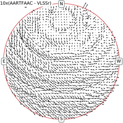
The position difference between the AARTFAAC WCS and VLSSr sources. The arrow lengths are 10 × the real sky distance. The mean position offset is 0.25°. The red circle is again the edge of the search area at Z = 50°.
4.2 Sky area, coverage, and sensitivity
However, this assumes that the given transient is detectable in every region across every image, which neglects the fact that for a wide-field instrument such as AARTFAAC, the transient sensitivity can vary across the field of view in a single image, and across images according to local sidereal and universal time. We can refine this by summing the total surveyed area as a function of sensitivity limit, allowing us to plot a continuous distribution that describes the surface density surveyed at each sensitivity (Carbone et al. 2016). In Fig. 3, we show this curve for the AARTFAAC survey (dark blue dashed curve), compared to many recent transient surveys across a wide range of frequencies and time-scales.

We compare the surface density to which we have probed for transients, that is, the 8σ detection limit, as a function of time-scale (left) and sensitivity (right), to a multitude of other recent surveys. Arrows denote upper limits placed by the survey, black stars mark reported transient detections. The diagonal lines in the right-hand panel have a power-law index of −3/2, expected of a population of standard candles uniformly distributed in Euclidean space, the red dash–dotted line is scaled to the surface density of the single potential extragalactic transient candidate discovered during this survey, and the grey lines scaled to the transient detected by Stewart et al. (2016), in steps of 103n, for integer n.
The survey sensitivity coverage is calculated from the parameters stored in the data base. Only information measured and calculated during each source extraction is stored, to reduce the data volume. Since the RMS noise and thus the sensitivity are slowly varying with position within the detection region, the survey data base does not store a noise map, but only the flux and detection signal-to-noise ratio of each source. We then of course know the RMS noise at each source location as the ratio of those numbers and can use those values to recreate a good noise map by interpolation. As a boundary value for the noise at the edge of the detection region for use in this interpolation we use the average of |$\rm RMS_{\mathrm{max}}$| and |$\rm RMS_{\mathrm{qc}}$|, which are the maximum RMS in the image and RMS in the region 20° around Zenith. Both values are calculated and stored by TraP during image processing. This approximation has been empirically verified by calculating the sensitivity area distribution directly from a set of 100 images across a 6 h observation.
4.3 Positive detections
Our survey revealed three populations of transient events, observable due to our fast imaging cadence.
4.3.1 Pulsar giant pulses
The first are extreme pulses from the pulsar B0950+08 (Kuiack et al. 2020). In the right-hand panel of Fig. 3, we show the surface density of these pulses detectable as a function of the sensitivity limit (magenta line). The distribution is the number of pulses of a given brightness, divided by the total sky area surveyed to that detection threshold. Since each pulse was detected blindly without prior assumption of a location, this fairly represents the surface density of such pulses, regarded as independent events in a population. For the astrophysical implications we must of course account for the fact that they all come from the same source, see Kuiack et al. (2020).
4.3.2 Isolated scintels
The second population of transients observed, indicated by the blue line in Fig. 3, do appear to be independent events. These are the spontaneous, singular magnifications of background sources, likely due to ionized plasma within the ionosphere of the Earth (Kuiack et al. 2021). The curve illustrates the brightness distribution of these ‘scintels’. They are time resolved, with widths typically in the range 10–100 s, and therefore we also plot their rate distribution as a function of time-scale in the left-hand panel of Fig. 3. Transient events of this class are also characterized by a time-frequency evolution that is inconsistent with an extragalactic dispersion delay.
4.3.3 Potential cosmic transients
Lastly, we observed a sample of transient events that do exhibit a time frequency evolution across the 4.2 MHz we observe, which could be consistent with dispersion delay due to propagation through the interstellar medium (ISM) and intergalactic medium (IGM). These candidates are summarized in Table 3. The candidates whose inferred dispersion measure (DM) is greater than the sum of the NE2001 ISM model (Cordes & Lazio 2002) and Galactic halo model (Yamasaki & Totani 2020) are shown above the dashed grey line in Fig. 4. These sources are more interesting to us because they can be more easily differentiated from the non-dispersed isolated scintels, singular magnifications due to near-Earth plasma, which typically have shorter (positive and negative) inter-frequency delays (Illustrated in fig. 10 of Kuiack et al. 2021).
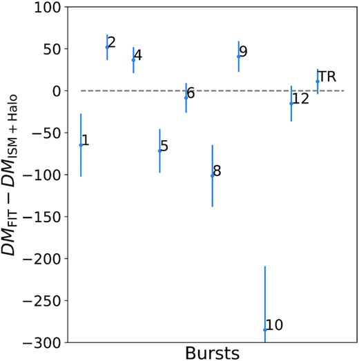
The inferred excess DM beyond the contribution from the Galactic ISM and halo. Sources below the zero line can be rejected as extragalactic transients, whereas those above could either be extragalactic or might be embedded in regions where the local ISM density is higher than predicted by the NE2001 model. We use a 20 per cent uncertainty in the model DM, which is much larger than our range.
Our sample of high interest transient candidates, defined as bursts with a large and negative inter-frequency delay, potentially corresponding to a physical dispersion delay. The Model DM is the sum of the NE2001 for the Galactic ISM and the halo model. The flux density given is the peak of the light curve, generated by measuring the integrated flux after dedispersing with the fit DM. Similarly, the width is the FWHM of the light-curve feature, after DM correction.
| Date Time | Label | RA | Dec. | |$\rm DM_{\rm model}$| | |$\rm DM_{\rm fit}$| | Flux density | Width |
|---|---|---|---|---|---|---|---|
| UTC | deg | deg | pc cm−3 | pc cm−3 | Jy | s | |
| 2017-02-25 03:21:27 | TR | 163.37 | 33.73 | 60 | 73 ± 3 | 80 ± 30 | 7.7 |
| 2017-02-25 04:19:11 | 2 | 215.16 | 26.75 | 56 | 108 ± 4 | 88 ± 24 | 42.6 |
| 2017-02-25 04:36:41 | 12 | 236.77 | 17.75 | 71 | 56 ± 7 | 100 ± 30 | 20.8 |
| 2018-09-23 04:48:13 | 1 | 36.66 | 26.85 | 82 | 18 ± 21 | 65 ± 26 | 33.5 |
| 2018-09-23 05:29:44 | 5 | 60.98 | 22.69 | 105 | 34 ± 5 | 62 ± 14 | 23.5 |
| 2019-01-01 03:42:16 | 9 | 147.22 | 41.11 | 67 | 108 ± 5 | 70 ± 30 | 32.4 |
| 2019-01-01 03:44:08 | 6 | 144.64 | 42.17 | 68 | 60 ± 4 | 67 ± 25 | 17.5 |
| 2019-01-01 03:47:45 | 4 | 157.74 | 34.39 | 62 | 99 ± 3 | 103 ± 20 | 22.1 |
| 2019-01-01 05:16:25 | 10 | 173.51 | 10.01 | 350 | 65 ± 6 | 75 ± 32 | 29.0 |
| 2019-02-03 01:22:58 | 8 | 186.33 | 25.90 | 154 | 53 ± 6 | 63 ± 24 | 51.8 |
We further differentiate this sample by comparing the relative effect that correcting the inferred DM has on the width and peak of the bursts. Intrinsically narrow pulses with large DM, such as FRBs, will see a greater increase in signal-to-noise ratio, as well as a reduction in the width, over the directly integrated bandwidth. Fig. 5 illustrates this. We see that for all of the candidates correcting the DM, |$\rm DM_{corr}$| decreases the pulse width and increases the peak, as expected. However, the candidate ‘TR’ is clearly an outlier. The pulse width is intrinsically much narrower than the others (Table 3).
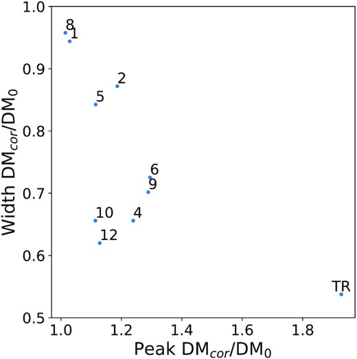
Here the effect of DM correction on each candidate is illustrated by plotting the ratio of the corrected to uncorrected burst width against the corrected to uncorrected burst peak height. Uncorrected width and peak are measured by integrating our 16 frequency bands without any frequency delay, i.e. |$\rm DM =0$|, the |$\rm DM_{\rm corr}$| corresponds to the best fit DM for each candidate. Intrinsically narrower busts with higher dispersion appear further down and to the right where our strongest candidate, labelled TR, is.
We illustrate this in more detail with the time-frequency plot for this outlier candidate in Fig. 6, which also contains additional transient signal after 03:24:36 UTC that is more consistent with the ‘usual’ ionospheric scintels. Though these appear near in time and space, they are clearly quite different in their characteristics. The first one is sharply defined and short in each sub-band, and the delay across the full band is larger than the width. The other two are much less sharp, lasting 30–40 s, and with a delay across the full band, if any, that is much less than the width, similar to the singular magnifications. In Fig. 7, we quantify this by showing the result of inferring a DM from time lag between the 16 sub-bands, measured by cross-correlating each sub-band with the highest frequency, for each candidate in Fig. 6. The first event (blue) has a tightly constrained delay curve, defined fairly sharply with a much lower uncertainty than the following two, as well as a value of the DM that matches the expectation for an extragalactic source in this sky location (Fig. 4).
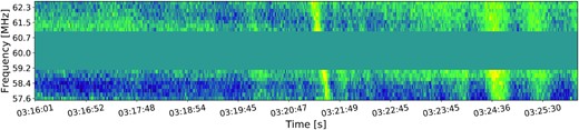
Time-frequency plot for the best extragalactic transient candidate detected during our survey (centre). The two sources following 03:24:36 are more consistent with scintels, given their lack of a well-defined dispersion delay, and time-scale, though no scintillating source is clearly associated (Fig. 8). Variation in the candidates flux density peak from 57.8 to 62.5 MHz is consistent with a flat spectrum after correcting for the time- and frequency-dependent background variation.
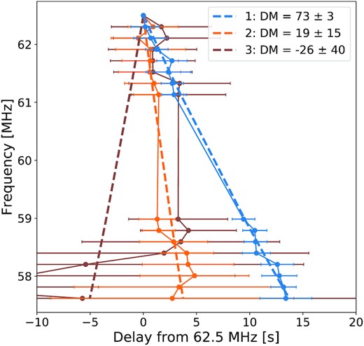
The frequency-dependent delay in the time of flux density peak for the three sources in Fig. 6, and the best-fitting DMs, and numbered in chronological order. Transient candidate 1 shows clear time-frequency dependence consistent with a dispersion delay, whereas candidates 2 and 3 do not.
Of course, this explanation implies that the occurrence of two ‘ordinary’ foreground scintels at the same location is a coincidence, and one might reasonably ask whether it is too much of one. To answer this, we first calculate the sky density of scintels during the time of the transient candidate ‘TR’, and find a chance alignment probability of magnifying plasma lens at the time of this candidate of 2 × 10⁻³ per second. During the 10 min illustrated in Fig. 6 one would therefore expect 1.3 ± 1 scintels, in fine agreement with the two observed. However, this agreement is somewhat undermined by a closer look at the image of this candidate (Fig. 8): there are no bright steady sources within the PSF of the transient (of the nearest sources within 1 deg, only one is greater than 1 Jy), so the scintels have to have magnifications of 200 or more. Such scintels are rare, more commonly the source being magnified is brighter and easily identified in the AARTFAAC data (Kuiack et al. 2021). Unfortunately we do not yet have good enough statistics of bright scintels to quantify this better, but on the whole the coincidence of the bright scintels with the candidate extragalactic source is somewhat uncomfortable. Finding a few more examples and/or better characterizing the likelihood and magnification distribution of scintillation storms will be needed to resolve this.
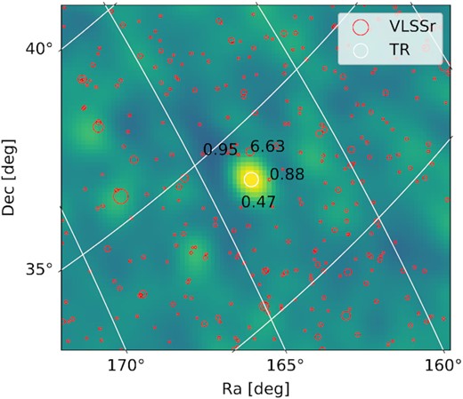
The image of the transient candidate at its peak flux density. The white circle radius corresponds to the position uncertainty. The red circles indicate VLSSr sources, with radii proportional to their flux density. The flux density of all VLSSr sources within a 1 deg radius from the transient candidate have their flux densities labelled.
5 DISCUSSION
Assuming our strong candidate, illustrated in Fig. 8, is a true extragalactic flare, we can search for potential associations within the position and distance uncertainty. With a best-fitting DM of 73 ± 3 pc cm−3, this DM would be extragalactic: in the direction of the source (RA 163.7 ± 0.5 deg, Dec. 33.8 ± 0.5 deg), the total Galactic DM is 30 pc cm−3 (Cordes & Lazio 2002), and the halo contribution is also 30 pc cm−3 (Yamasaki & Totani 2020). This places the source origin definitely outside the disc of our Galaxy and likely outside of the halo (but, given local variability of sight-lines relative to the DM models, not with very great certainty). Using the DM-distance relation for the IGM, DM = 900z pc cm−3 (McQuinn 2014; CHIME/FRB Collaboration 2019b) gives a redshift value of 0.015, or distance of 63 Mpc (Wright 2006). Given that the foreground DM value is uncertain and that there might be also a contribution from the environment or host of a putative extragalactic event, we should regard this value as indicative of the upper limit to the distance rather than a measured value.
In the Advanced Detector Era (GLADE, v2.3) catalogue of nearby galaxies (Dálya et al. 2018), there are three potential galaxies within the position uncertainty and distance limit: PGC2039259 at 26.4 Mpc, NGC 3442 at 27.96 Mpc, and PGC032706 at 55.83 Mpc, all with flux densities of 0.5 Jy or less. None of these is detected in our AARTFAAC data, so if the flare originates from one of them, its radio luminosity is more than 200 times that of the quiescent galaxy’s total value. Since we cannot identify the event with a quiescent source, the cause of this flare remains rather speculative at the moment. To set the scale, at a distance of 50 Mpc this flare has a peak radio luminosity (assuming a spectral range of 100 MHz and isotropic emission) of 3 × 1037 erg s−1 and emitted energy only in the radio band of 3 × 1038 erg. By the usual argument of how fast a radio flare can rise from a source of a given size (e.g. Pietka et al. 2015), this implies a brightness temperature in excess of 1034 K. Even if we do assume the source is on the outskirts of the Galaxy, at 50 kpc, the implied brightness temperature would still be 1028 K. In either case, the emission mechanism underlying this phenomenon then needs to be coherent. This also means the radiation is very likely beamed and thus the stated luminosities and energies are upper limits.
Given these rather strong implications, we prefer to regard this event as a candidate extra-Galactic event for now, and await the discovery of a few more confirming cases and better understanding of the outliers in the frequency-time delay distribution of the magnification events.
Our survey places constraints at shorter time-scales and with a very large survey volume, to a depth that is however less than most other surveys. Our results are broadly consistent with other low-frequency surveys, which report mostly upper limits to the rate of radio transients below 200 MHz, at time-scales below 1 min (Obenberger et al. 2015; Rowlinson et al. 2016; Anderson et al. 2019). These three works, together with ours, place similar limits on the brightness of a hypothetical population of isotropically distributed, standard candle, transient events. But we shall now compare them in more detail for consistency also with some detections in this frequency range, by taking these differences into account.
We have observed a single example of a potential transient, with a flux density of 80 ± 30 Jy and lasting 7.7 s, and a dispersion delay across our frequency range indicative of an extragalactic origin. If this transient is a member of a population of sources that is isotropic on the sky and uniform in space density, the observed power-law brightness distribution (log (N > S) ∝ S−p) of such a population would have a so-called Euclidean index p = 3/2. That theoretical brightness distribution is plotted as the red dash–dotted line in the right-hand panel of Fig. 3. One previous upper limit lies below this line, from the 28 s-time-scale MWA survey by Rowlinson et al. (2016), at 182 MHz. However, to see whether this indicates a flatter than Euclidean brightness distribution we must account for the fact that our transient is shorter than the 28 s cadence of the MWA survey. The fluence of our transient was 580 ± 150 Jy s, and so its flux averaged over a 28 s time bin was 20 ± 6 Jy. If we use that value and p = 3/2 to extrapolate to the sensitivity threshold of 0.285 Jy of the MWA survey, we predict a surface density of 2.4 × 10⁻⁷ deg−2, somewhat below their upper limit of 4.1 × 10⁻⁷ deg−2. Their upper limit is thus consistent with our detection. (Note we have taken the optimistic view that the event would fall entirely within one MWA time bin; more realistically it would be split over two and this would further reduce the detection probability, see Carbone et al. 2016.) The MWA survey was at a three times higher frequency than ours, so this marginal consistency implies that if our source is part of Euclidean flux distribution, it cannot have a strongly rising, self-absorbed, spectral index between 60 and 182 MHz.
The population of extreme-fluence pulses from PSR B0950+08 (Kuiack et al. 2020) is of course entirely from one source, and so the rate or surface density averaged over the sky should be taken with a grain of salt. Also, this pulsar is very nearby (DM = 3.0 pc cm−3) and thus is not dispersed enough for the pulse to be smeared over multiple time bins across our band. Most other known giant-pulse emitting pulsars have rather higher DM, and we are now searching our data with de-dispersion to their known DMs in order to see whether this phenomenon extends to other pulsars.
The population of isolated magnifications of background sources, due to turbulent ionized plasma in the ionosphere-plasmasphere region (Kuiack et al. 2021), has an effective surface density that agrees well with the non-detection by Anderson et al. (2019), given the rate and time-scale probed. Many characteristics of the cosmic transient detected by LWA1 and LWA-SV (Varghese et al. 2019), including time-scale, burst shape, and brightness, fit this population well. Although the rate is somewhat larger than our distribution would predict, this could be consistent with the fact that a plasma lensing is stronger at lower frequencies (e.g. Clegg, Fey & Lazio 1998), and the LWA1/LWA-SV survey was conducted at 34 MHz. The non-detections of this particular phenomenon by both Obenberger et al. (2015) and Varghese et al. (2019) are consistent with the distribution we see. While the survey by Obenberger et al. (2015) probes a very large volume at 60 MHz, it did not have the sensitivity required. And Varghese et al. (2019), which was much more sensitive at the same frequency, searched insufficient volume, for the time-scale analysed.
Stewart et al. (2016) detected a single transient event with a flux density of 15–25 Jy in a survey that used 2149 snapshots of 179 square degrees each around the North celestial Pole, each lasting 11 min. Given the positive detection and surveyed volume, the rate was determined to be |$3.9^{+14.7}_{-3.7}\times 10^{-4} ~\mathrm{d}^{-1}\mathrm{deg}^{-2}$|. If we translate this rate to our typical sensitivity limit of 60 Jy with a Euclidean source count distribution, N(> S) ∝ S−3/2, we expect about eight similar events in the volume of our survey. This means that our non-detection has quite a low probability, 2.8 × 10⁻⁴, under the Euclidean assumption. Since the frequencies of the two surveys are the same, spectral index cannot be a confusing issue here and so we conclude that between 15 and 60 Jy, the source counts for this population must be quite a bit steeper than Euclidean, p ≤ −2.5. Our next survey, which uses an additional six LOFAR stations and has a 10 times better sensitivity (light blue dashed curve in Fig. 3) does go down to below the flux level of the Stewart et al. (2016) transient and should therefore detect this population.
The detection of FRBs at the lowest frequencies remains an important goal for constraining the rate and spectral shapes of these events, and thereby perhaps their origin and emission mechanism. Therefore, we evaluate to what degree our survey is sensitive to the brightest tail end of the FRB population. While FRBs have been detected between 110 and 188 MHz with LOFAR (Pleunis et al. 2021), these originated only from FRB 20180916B, a single repeating FRB. We therefore use the all-sky FRB rate measured by CHIME (CHIME/FRB Collaboration 2019a), who have reported detections of many single and repeating FRBs across the Northern hemisphere detected at frequencies down to 400 MHz, the bottom of the CHIME bandpass. The all-sky rate they give is 300 d−1 above a flux density limit of 1 Jy, consistent with the value of 400 d−1 by Connor et al. (2016). The observing frequencies are too different to neglect, but since FRB spectra have a wide range of measured slopes (Petroff, Hessels & Lorimer 2019, and references therein), both rising and falling to higher frequencies, we cannot do much better than assume a flat spectrum. Next, we must scale the sensitivity threshold for the burst peak flux density to 60 kJy. This results from our 1 s integration, with an average 1 ms intrinsic burst width. On the bright end of the distribution, the FRB rate seems to follow R(> F) ∝ F−2.2 (Petroff et al. 2019). Therefore, the expected rate of FRBs greater than 60 kJy is 9 × 10⁻⁹ d−1sky−1, which translates to a surface density per snapshot of 2.6 × 10⁻¹⁸ deg−2; this yields a completely negligible 2 × 10⁻⁸ expected FRB detections in our survey. It is therefore not surprising that we did not detect any FRBs, even if we optimistically assumed a fraction of them to have steep spectral indices, especially since we also neglected the deteriorating effect of dispersion smearing.
6 CONCLUSIONS
We have presented results of the first survey with the AARTFAAC instrument for rare, bright, and fast radio transients at 60 MHz and shown for the first time two significant-sized populations of such radio transients: extreme pulses from the nearby pulsar B0950+08 and strong, short-duration magnifications of known radio sources caused by space weather, as well as a single candidate extragalactic transient, possibly the first of another class of transient. We set a strong upper limit of about 1.1/sky/d to any yet undiscovered types of transient with peak fluxes above 60 Jy and durations of seconds to minutes. We also discuss the power of our survey to constrain the bright end of the FRB population, and find that this is very little. But in the case of the enigmatic 5 min transient found by Stewart et al. (2016), we can constrain the slope of the brightness distribution to be much steeper than Euclidean because we did not detect any such transients. However, since by far most false positives in our search come from detections in only one band, because RFI is typically narrow band (see Table 2), we have to reject all narrow-band sources. Therefore, if these transients are also narrow-band, they could only be constrained from a site with much lower RFI or a search with narrower frequency channels. Finally, we set very low upper limits to the surface density and rate of any other, yet unknown types of low-frequency radio transient.
We also find one case of a 7.7 s, 80 Jy flare that shows all the hallmarks of being dispersed, with a DM that likely puts it at extragalactic distance, or at the very least in the outskirts of our own Galaxy. We find no underlying radio source brighter than 0.5 Jy. We withhold final judgement on whether it really is dispersed until we have collected more events, since there are some outliers in the distribution of magnification events that have similar time delays to this event. If it is indeed a distant source, its emission is quite extreme, requiring a brightness temperature of 1028–34 K.
There are still quite a number of steps of improvement possible: first, we have about as much 6-station AARTFAAC data yet to be analysed as we report here, and we can search the data with crude de-dispersion in order to look for pulses like those of B0950 in other pulsars. Furthermore, we have calibrated the new 12-station AARTFAAC and performed a first short survey with it (Shulevski et al. 2021), and are about to embark on a much longer survey with this roughly 10 times more sensitive array. This should, for example, allow us to detect a population of sources like the one found by Stewart et al. (2016) and expand on, or disprove, the existence of fast extragalactic transients like our current candidate; and perhaps it will unveil more unknown unknowns.
ACKNOWLEDGEMENTS
AARTFAAC development and construction was funded by the ERC under the Advanced Investigator grant no. 247295 awarded to Prof. Ralph Wijers, University of Amsterdam; This work was funded by the Netherlands Organisation for Scientific Research under grant no. 184.033.109. We thank The Netherlands Institute for Radio Astronomy (ASTRON) for support provided in carrying out the commissioning observations. AARTFAAC is maintained and operated jointly by ASTRON and the University of Amsterdam.
We would also like to thank the LOFAR science support for their assistance in obtaining and processing the data used in this work. We use data obtained from LOFAR, the Low Frequency Array designed and constructed by ASTRON, which has facilities in several countries, that are owned by various parties (each with their own funding sources), and that are collectively operated by the International LOFAR Telescope (ILT) foundation under a joint scientific policy.
This research made use of Astropy,2 a community-developed core Python package for Astronomy (Astropy Collaboration 2013) (Price-Whelan et al. 2018), as well as the following KERN (Molenaar & Smirnov 2018), Pandas (McKinney 2010), NumPy (van der Walt, Colbert & Varoquaux 2011), and SciPy (Jones et al. 2001). Accordingly, we would like to thank the scientific software development community, without whom this work would not be possible.
DATA AVAILABILITY
The data underlying this article can be shared on reasonable request to the corresponding author. Additionally it some data products are available through the Zenodo open-acces data repository DOI:10.5281/zenodo.4778360.
