


ABSTRACT
Identification of anomalous light curves within time-domain surveys is often challenging. In addition, with the growing number of wide-field surveys and the volume of data produced exceeding astronomers’ ability for manual evaluation, outlier and anomaly detection is becoming vital for transient science. We present an unsupervised method for transient discovery using a clustering technique and the astronomaly package. As proof of concept, we evaluate 85 553 min-cadenced light curves collected over two ∼1.5 h periods as part of the Deeper, Wider, Faster program, using two different telescope dithering strategies. By combining the clustering technique HDBSCAN with the isolation forest anomaly detection algorithm via the visual interface of astronomaly, we are able to rapidly isolate anomalous sources for further analysis. We successfully recover the known variable sources, across a range of catalogues from within the fields, and find a further seven uncatalogued variables and two stellar flare events, including a rarely observed ultrafast flare (∼5 min) from a likely M-dwarf.
1 INTRODUCTION
In the era of large time-domain surveys, classification and discovery of transient sources is becoming reliant on machine classification to handle the associated large amounts of data. Current ground based surveys such as the Zwicky Transient Facility (ZTF; Bellm et al. 2019; Graham et al. 2019), Dark Energy Survey (Dark Energy Survey Collaboration 2016), and the All Sky Automated Survey for Supernovae (Shappee et al. 2014) are able to scan thousands of square degrees continuously, which amounts to petabytes of data annually, and recently the Panoramic Survey Telescope and Rapid Response System Survey (Stubbs et al. 2010; Chambers et al. 2016) delivered the first petabyte scale optical data release. Space-based time-domain missions have provided unprecedented volumes of photometry, light curves, and proper motions for Galactic sources, with Kepler (Borucki et al. 2010) and K2 (Howell et al. 2014) targeting ∼400 000+ individual stars, TESS (Stassun et al. 2018) is expected to target at least 200 000 sources producing light curves for each source, and Gaia has already released almost 2 billion sources. Overcoming the mining challenges of these increasing amounts of data to not only identify and catalogue the multitude of known transient types but to make discoveries of new or anomalous sources is paramount to the success of future large transient surveys and time-domain science.
1.1 Supervised learning
Supervised machine learning has already been utilized extensively by several surveys and teams in astronomy for identification of variable stars and quasi-stellar objects from light curves via multivariate Gaussian mixture models, random forest classifiers, support vector machines, or Bayesian neural networks (Debosscher et al. 2007; Kim et al. 2011; Richards et al. 2011; Bloom et al. 2012; Pichara et al. 2012; Pichara & Protopapas 2013; Kim & Bailer-Jones 2016; Mackenzie, Pichara & Protopapas 2016). The literature aforementioned successfully shows the robustness of source classification while using the combination of supervised algorithms trained on extracted features. Features represent a set of measurable properties/characteristics of the light curves being studied (discussed in further detail in 4.1). The most common features used in earlier works are available within the python package fats by Nun et al. (2015).
Classification of non-folded light curves of extragalactic transient sources has also been explored, moving away from selecting the class of the object by fitting analytical templates built from a set of known sources (Richards et al. 2011; Karpenka, Feroz & Hobson 2012; Lochner et al. 2016; Möller et al. 2016; Narayan et al. 2018). While these techniques work well for catalogues of light curves, they cannot easily be applied to real-time data.
Real-time classification of supernovae by Muthukrishna et al. (2019) and Möller & de Boissière (2020) has shown the effectiveness of deep recurrent neural networks, without the need to rely on extracting computationally expensive features of the input data.
1.2 Unsupervised learning
Even with machine learning advances in astronomy, mining data for unknown or anomalous events is relatively unexplored, as the majority of current algorithms require training data sets of known events. Mackenzie et al. (2016) developed an unsupervised feature learning algorithm that takes subsections of variable star light curves to cluster and use as features to train a linear support vector machine. This work eliminates the need for traditional feature extraction, limiting the computing time and biases associated with feature selection. Only limited work into actual transient classification or anomaly detection via unsupervised means has been performed within time domain astronomy.
Valenzuela & Pichara (2018) performed unsupervised clustering of variable star light curves by creating variability trees using the k-medoids clustering algorithm of fragmented light curves. This method offers a novel and computationally fast approach to data exploration but is again limited by the need for known light curve examples for similarity searches. To identify Kepler data outliers for visual inspection, Giles & Walkowicz (2019) performed light-curve clustering using Density-Based Spatial Clustering of Applications with Noise (DBSCAN). They report the successful extraction of the known anomalous Boyajian’s star via their method; however they identified that the DBSCAN assumption of constant density clusters is a limitation. It should be noted that the overwhelming majority of work performed to date on light-curve classification by machine learning has used 30 min to several day cadence, including folded light curves.
Mahabal et al. (2017) presents another approach to light-curve classification, by reducing the time series data to 2D representation in order to classify them using deep learning techniques. This approach maps the change and magnitude over time to create a visual representation of the light curve as an image to be used in the deep learning process. This method presents an alternate approach of unsupervised learning for time-series classification without the need for feature extraction.
1.3 Anomaly detection in fast cadenced surveys
Currently, the majority of wide field optical surveys explore a limited region of the luminosity-time-scale phase space, with an average cadence of hours to days between visits to fields, with only a few programs exploring the phase space shorter than 1-h cadence (see Lipunov et al. 2004,2007; Roykoff et al. 2005; Rau et al. 2009; Berger et al. 2014; Burdge et al. 2019; Richmond et al. 2020). What is largely unexplored by these surveys is the phase space of transient events occurring on seconds-to-minutes time-scales. There are several events expected to occur on these time-scales, and understanding both the events and the general nature of the fastest transients in the Universe is crucial for understanding the transient Universe as a whole. For example, the upcoming Rubin Observatory Legacy Survey of Space and Time (LSST) is predicted to generate nearly 10 million transient alerts each night. As such, it will be invaluable to quickly and meaningfully quantify the expected large volume of short time-scale events to help assist in follow-up priority assignment (LSST Science Collaboration 2009). To do so, the astronomical community will rely heavily on the use of brokers and their integrated algorithms serving alert streams. Current brokers, which include alerce,1antares,2lasair,3 and mars4 are already in use on the nightly ZTF stream, successfully identifying known extragalactic and galactic transient and variable events. However identifying anomalous events can prove challenging with pre-trained algorithms, especially within the rarely explored fast time-scales (seconds-to-minutes).
The multiwavelength Deeper, Wider, Faster (DWF) program offers the ability to explore optical transient events with the depth and cadence required to enable the quantification and characterization of Galactic and extragalactic variable and fast transient rates for current and upcoming large-area searches and surveys and to similar depths as 4m–8m class telescopes. Such as gravitational wave counterpart searches, the Rubin Observatory LSST survey, and others. This work presents our effort to explore the DWF optical data for anomalous light curves without the restrictions of prior assumptions or expectations.
As our literature review highlights, the vast majority of work to date on machine learning for transient classification and identification has relied on pre-existing understanding of longer duration variable and transient time-series behaviour. In this work, we demonstrate an unsupervised method to aid in the discovery of both known and poorly understood transients on the time-scales of seconds-to-minutes.
The paper is organized as follows: A brief introduction to the DWF program is presented in Section 2, two DWF data gathering strategies and the data in Section 3. We present our multifaceted anomaly detection approach in Section 4 and our proof of concept results in Section 5. We conclude by presenting our overall outcomes in Section 6.
2 THE DEEPER, WIDER, FASTER PROGRAM
Several new and exciting astronomical fast transient events have been discovered in recent decades and the progenitors and physical mechanisms behind many of them are still poorly known (e.g. Fast Radio Bursts, FRBs), supernova shock breakouts, Fast-Evolving Luminous Transients (FELTs), and other rapidly evolving extragalactic events (for example: Lorimer et al. 2007; Garnavich et al. 2016; Perley et al. 2018; Prentice et al. 2018; Rest et al. 2018). What has limited our ability to detect and understand these events is the capability to gather data in short, regular time intervals before, during and after the events; as well as over a range of wavelengths. The DWF program (Andreoni et al. 2017a, b; Meade et al. 2017; Vohl et al. 2017; Andreoni & Cooke 2018) has been designed with these challenges specifically in mind, constructing an all wavelength and simultaneous observational program of over 70 facilities to date. DWF takes a ‘proactive’ approach to transient astronomy, with coordinated simultaneous wide-field fast-cadenced multiwavelength observations of target fields taken continuously over 1–3 h periods, capturing data before, during, and after the transient events. The optical data collected during the simultaneous observations is processed in near real-time to quickly identify candidates requiring the use of rapid Target of Opportunity (ToO) observations.
DWF unites the worlds most sensitive facilities with large fields of view in the optical – the Dark Energy Camera (DECam; Flaugher et al. 2015) on the Cerro Tololo Inter-American Observatory (CTIO) Blanco 4-m telescope in Chile and Hyper-SuprimeCam (HSC; Miyazaki et al. 2017) on the Subaru 8-m telescope in Hawaii – taking continuous 20–30 s exposures. Using this strategy, DWF is able to explore a region of luminosity phase space rarely explored by many traditional surveys (see Andreoni et al. 2020). From the real-time data processing, DWF can quickly identify candidates and coordinate rapid-response and long-term follow-up observations of transient candidates. DWF began in 2014 and since its inception has had two pilot runs and seven operational runs (see Andreoni & Cooke 2018; Cooke et al., in preparation).
The unique design of DWF allows exploration of transients on the seconds-to-hours time-scales, providing further understanding into known classes of fast transients, events theorized to occur on these time-scales, and very early detections of slower evolving events (see Section 3 for observation specifics). Using either DECam or HSC, the deep optical component of DWF can explore a region of parameter space not yet reached by previous transient surveys. Note that, although DWF collects simultaneous fast-cadenced data across all wavelengths, radio through gamma-ray, from multiple facilities, we will only focus on DECam optical data here. Work by Andreoni et al. (2020) utilized the unique DWF data and ‘Mary’, our transient difference image discovery pipeline, to detect both galactic and extragalactic transients on the minute time-scales. In this paper, we examine light curves generated purely from science images (i.e. without image subtraction) for all sources in our chosen fields, and explore the ability to identify known and unknown transient and variable sources through the use of unsupervised machine learning. By examining every source light curve through an unsupervised algorithm, we aim to not only distinguish clear source separations in feature space, but identify and classify unknown and outlying sources to comprehensively explore fast transient events and source variability on the seconds-to-hours time-scales.
3 DATA
We use fast cadenced data collected during DWF runs using DECam. We collect 20 s, continuous imaging of targeted fields, acquired in a single band, the ‘g’ filter. We choose the continuous use of the ‘g’ filter to maximize depth with DECam, reaching ∼0.5 magnitudes deeper in comparison to the other filters in dark time. The expected limiting magnitude in ‘g’ band is m(AB) ∼23, for an average seeing of 1.0 arcsec and airmass of 1.5 (relatively high airmass due to the field constraints of observing simultaneously with multiple facilities). For this work, the DECam images are post-processed through the NOAO High-Performance Pipeline System (Scott et al. 2007; Swaters & Valdes 2007; Valdes & Swaters 2007) and then transferred to the OzSTAR supercomputer at Swinburne University of Technology for our data analysis. The DECam 62 CCD mosaic is separated into individual fits files for each extension. Each CCD is processed separately for source extraction using SExtractor (Bertin & Arnouts 1996) and all source magnitudes are corrected for exposure time and magnitude offsets against the SkyMapper Data Release 2 catalogue (Bertin & Arnouts 2010; Onken et al. 2019). A master list is compiled by cross-matching all extracted sources from each CCD, over all exposures within 0.5 arcsec radius between source centroids into one catalogue of source positions. This master catalogue is used to create light curves for each source, replacing any non-detections per single exposure with the CCD exposure detection upper limit represented in the light curve.
To date, DWF has targeted 20 separate fields, each observed typically for six consecutive nights, and has accumulated over 1 million source detections. In this work, we analyse light curves from two separate fields for only one night each, observed using two different observing strategies. In Section 5.1, we analyse data collected from the DWF ‘J04-55 field’ on 2015 December 18, using a field centre of RA:04:10:00.0 and DEC: −55:00:00.0. The continuous 20 s exposures were collected over a 90 min period, using a stare’ observational strategy (i.e. pointing at the same coordinates with no small field dithering between exposures). In Section 5.2, we analyse data gathered over an 80 min period of continuous 20 s exposures centred on the ‘Antlia field’ RA: 10:30:00.0 and DEC: −35:20:00.0 on the Antlia cluster of galaxies. These data were collected on 2017 February 6 and utilized a five point dithering strategy at the beginning, middle, and end of the observation, while staring in between. In these data, we explore the contribution of telescope dithering to the false positive rate of anomaly detection in Section 5.2.
4 METHODOLOGY
We use the following methodology: (1) feature extraction, (2) clustering, (3) t-SNE visual representation, (4) anomaly ranking and visualization with astronomaly. We use feature extraction to find a low dimensional representation of the data, clustering to eliminate large clusters of ordinary objects and instrumental effects and isolate possible interesting transients, anomaly detection to rank these remaining objects by ‘abnormality’ and finally astronomaly to visually explore the detected anomalies. Note that all stages are performed on nightly light curves with an average cadence of ∼60–68 s between light-curve points, accounting for both the 20 s exposure and 40 s CCD readout time, CCD clear and rest. We utilize python for all stages, using the following packages scikit-learn, hdbscan, fats, astropy, numpy, pandas, and matplotlib (Hunter 2007; McKinney et al. 2010; Pedregosa et al. 2011; Nun et al. 2015; Oliphant 2015; McInnes, Healy & Astels 2017; Price-Whelan et al. 2018).
4.1 Features
As the number of data points differ for different light curves, we extract a uniform set of features to (i) reduce the dimensionality, and (ii) allow for direct comparison between light curves that may be on different time-scales with different sampling properties. To represent our unique fast-cadenced data, we use a mixture of normalized features developed and used primarily for the identification of variable stars and quasi-stellar objects. We performed principle component analysis on the features and selected those that corresponded to large eigenvalues. The majority of our features are taken from work by Richards et al. (2011), which were used to classify variable stars from sparse and noisy time-series data. We use only the features not restricted explicitly to folded light curves or periodic sources. Some examples of the features used are amplitudes, standard deviation, linear trend, maximum slope, etc. In addition to these, we used the stellar variability detection features, H1 (amplitudes), R21 (the 2nd to 1st amplitude ratio), and R31 (the 3rd to 1st amplitude ratio) which are focused around Fourier decomposition. The remaining features were taken from work in quasi-stellar object selection, these being autocorrelation length, consecutive points, variability index, and Stetson KAC as used by Kim et al. (2011) and mean, σ and τ taken from a continuous autoregressive model fitted to our data from Pichara et al. (2012). We extract 25 unique features from each light curve using mostly using fats and some in-house routines. Full details and sources for the features used are shown in Appendix A1.
In this work, we run feature extraction in parallel on the OzSTAR supercomputer at Swinburne University. We utilize the Intel Gold 6140 18-core processors on OzSTAR, achieving a feature extraction speed of ∼110 s per 1000 light curves when processed serially.
4.2 HDBSCAN
The focus of this paper is to use machine learning to analyse and cluster our light curves. We choose to use Hierarchical Density-Based Spatial Clustering of Applications with Noise (HDBSCAN5; McInnes et al. 2017). The theoretical method behind this algorithm was first proposed by Campello, Moulavi & Sander (2013). HDBSCAN takes the approach of Density-Based Spatial Clustering of Applications with Noise (DBSCAN) and converts it into a hierarchical clustering algorithm by varying the value of epsilon (ϵ) to identify clusters of varying densities (for further details see McInnes et al. 2017).
To better understand how HDBSCAN works, we first outline the original DBSCAN algorithm by Ester et al. (1996). DBSCAN performs nearest neighbour searches in a given feature space to determine clusters of overdensities, points closely related in distance, and identify outlier points that exist in low density regions as noise. DBSCAN requires two parameters, ϵ, which represents the radius of the neighbourhood search and a minimum number of points (minPts), which must exist in a neighbourhood to constitute a dense region. What has limited the use of DBSCAN in the past is the inability to vary ϵ in a given data set, requiring clusters to have similar densities. However, HDBSCAN can take in a minimum cluster size parameter which eliminates the need for a single value of ϵ when determining clusters from a dendrogram, adjusting of ϵ as it explores clusters of varying densities.
After several preliminary tests combining the different distance metrics and varying minimum cluster sizes to evaluate cluster purity and uniformity, we opted to require a minimum cluster size of 5 and to use a Euclidean distance metric for its intrinsic ability to calculate the shortest distance between points. We aim to create as many distinct clusters in our feature space as the algorithm will allow to limit the outliers to very low density regions.
4.3 t-SNE
To help visualize the clustering of objects in our high dimensional feature space, we use the t-distributed Stochastic Neighbor Embedding (t-SNE) algorithm developed by van der Maaten & Hinton (2008). The t-SNE algorithm uses the same Euclidean distance metric to measure the proximity of all features in higher-dimensional space. It converts these distances to probabilities using a Gaussian distribution. A similarity matrix of the probabilities is stored for the higher-dimensional space, and the feature space is then collapsed down to 2 or 3 dimensions, depending on the user’s choice, where the Euclidean distance is calculated once again using a t-distribution to assign probabilities and saved as a second similarity matrix. The two distributions are then minimized using the sum of Kullback–Leibler divergence of all data points using a gradient descent method to return a 2D representation of the distance of data in our feature space. It is important to note that due to the stochastic nature of t-SNE, it is used here only for visualization and not cluster identification. We note here that t-SNE was performed for the entirety of our data sets, using the OzSTAR6 computing nodes as well as on a personal machine with 8 GB ram and a 4.0 GHz quad-core Intel Core i7. We acknowledge that for future work the use of Uniform Manifold Approximation and Projection for Dimension Reduction (UMAP; McInnes, Healy & Melville 2018) is a promising method for dimensionality reduction, however in this work we were unable to use UMAP due to computational issues and we deemed t-SNE to be sufficient.
4.4 astronomaly
To find the most anomalous light curves, in each cluster, we use the python package astronomaly7 (Lochner & Bassett, in preparation) which is comprised of a python back end and JavaScript front end to easily explore the data via a locally hosted web interface (for further details see Appendix B1). astronomaly is a flexible framework, designed to detect anomalies within astronomical images or light curves using any of a variety of anomaly detection algorithms. Here we use the scikit-learn implementation of isolation forest (Ting, Liu & Zhou 2008) available in astronomaly. Each cluster of light curves identified by HDBSCAN was saved in individual data frames containing each light curve’s features.
Using astronomaly, each cluster’s light curve’s were evaluated independently, feeding both their features and original light-curve file into the back end of the package.
The isolation forest then works to isolate each light curve by recursively generating partitions, creating a tree structure ultimately segregating each light-curve point into nodes. Each node either contains one individual data point, or several data points all with the same feature value.
The web interface GUI allows the user to visually inspect the highest ranking anomalous light curves (as measured by the isolation forest algorithm), as well as explore the interactive t-SNE plot to probe the lower dimensional cluster space. To enable more rapid visualization, for this work we limit astronomaly to present only the 2000 most anomalously ranked light curves in the GUI interface.
astronomaly serves two purposes in this work. The first is easy visualization of the data in the clusters. Each cluster is analysed individually and the interactive t-SNE plot allows the user to quickly determine if the objects in the cluster do indeed look similar. The data can then be further vetted using the ranked anomaly system. The most anomalous objects within the cluster will appear first and hence should be the objects that are least likely to actually belong to that cluster. Thus, the effectiveness of the clustering can be quickly evaluated without the need for exhaustive study of every single light curve in the cluster.
The second reason we use astronomaly is to identify anomalous sources in the ‘unclustered’ group. With the same ranking system, the most interesting sources (and also instrumental effects) should appear early in the list allowing quick identification. It is critical to note that while this data set is still small enough to manually investigate every object (especially with astronomaly’s visual interface), for data sets consisting of millions of light curves, this would simply not be possible and the automated ranking becomes much more important to allow rapid discovery of anomalous sources.
5 RESULTS
5.1 DWF J04-55 field – no dithering observational strategy
We present the results of our unsupervised method applied to light curves over a 90-min observation of the DWF ‘J04-55 field’ using DECam in stare mode (the telescope tracked the same field centre coordinates for the duration of the observations). It is important to acknowledge that small movements of the telescope may still be present due to telescope guiding, shutter movements, and small pointing shifts. A total of 89 images were acquired, with 23 199 sources, as identified in the J04-55 field from the 5-night master source list, as having greater than three detections (Ndet > 3) for feature extraction.
5.1.1 Clusters
A total of three clusters were identified using HDBSCAN, as shown in Table 1. Cluster 2 dominates, containing |$98.7{{\ \rm per\ cent}}$| of light curves in the field. Inspection showed that this cluster overwhelmingly contained sources which were unchanging in magnitude, consisting of both stars and galaxies. In such a short time-scale observation, we expect that the majority of sources will be assigned to a single cluster in this manner. The two remaining clusters identify faint sources only breaching the detection threshold a few times during the 90 min, and sources near, or on, the edges of CCDs which have caused unusual/anomalous light curves. A visual representation of the clusters in feature space can be seen in Fig. 1.
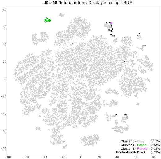
Feature space of the 25 features of the 23 199 light curves of the ‘J04-55 field’ collapsed down to 2 dimensions using t-SNE with the clusters labelled in Table 1 and coloured accordingly. It is important to note (1) that the axis values within a t-SNE are not physically meaningful and hence not labelled, and (2) that the t-SNE algorithm works by adapting its own notion of distance to regional density variations in the higher dimensional data. As a result, t-SNE naturally expands dense clusters and contracts sparse ones when collapsed as shown, and this can make some structure within the t-SNE plot appear more significant than it is.
The details of each of the three clusters identified by the HDBSCAN algorithm. The description of the light curves refers to both the light curve and information gathered from individual cutouts of the detection images. Unclustered represents light curves unable to be identified to a cluster.
| Description of light curves | Cluster ID | # of Light curves | Per cent of Sources |
|---|---|---|---|
| Faint sources | Cluster 0 | 8 | 0.03 per cent |
| at detection | – | – | – |
| threshold | – | – | – |
| Sources near | Cluster 1 | 144 | 0.62 per cent |
| CCD edge | – | – | – |
| Steady light curves | Cluster 2 | 22 909 | |$\gt 98.7$| per cent |
| Real and | Unclustered | 138 | <0.59 per cent |
| photometrically | – | – | – |
| affected light curves | – | – | – |
5.1.2 Variable/transient sources
A total of 138 light curves remained unclustered (referred to as noise by HDBSCAN, shown in black on Fig. 1). The unclustered light curves represent those which have a significant distance from identified clusters and represent the outliers in the data. It is these outliers which are variable and transient sources in the field. The light curve of each was visually inspected (in order of anomaly score) using the astronomaly package and variable sources were cross-matched to existing catalogs to check for known variability (mainly the International Variable Star Index (VSX) catalogue (Watson, Henden & Price 2006), identified RR lyrae stars from the Dark Energy Survey (DES) Stringer et al. (2019), and the Catalina Surveys Southern Periodic Variable Star Catalogue (Drake et al. 2017)). For newly discovered sources showing variability, locations on a Colour–Magnitude Diagram (CMD) were calculated using Gaiadata release 2 parallax and photometric information (Evans et al. 2018; Luri et al. 2018). The CMD positions were then overlaid on the variability CMDs presented in work by Gaia Collaboration (2019) and shown in Appendix C1 as green triangles. After evaluation with astronomaly, it was determined that the majority of the light curves were indeed anomalous in structure, however caused by instrumental and observational effects. The false positives represented sources on the edges of CCDs or those teetering on the detection threshold. However we did identify six sources of continuous variability, five of which have been previously catalogued, with the remaining variable source discovered by this work. In addition to the variable stars, a stochastic classical flare event was also identified. Source IDs, name, coordinates, known catalogue ID (if available) and period are shown in Table 2, and the light curves are shown in Fig. 2.
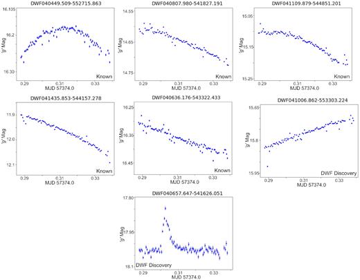
Four previously known and two newly discovered variable/transient sources present in the unclustered noise within the J04-55 field analysis.
Sources identified showing variability in J04-55 and Antlia fields. Note: lines in bold indicate discoveries in this work.
| Field | DWF ID | Catalogued ID | Typea | Period (d)b |
|---|---|---|---|---|
| J04-55 | DWF040449.509-552715.863 | ASASSN-V J040449.48-552715.9 | W Ursae Majoris | 0.27 |
| J04-55 | DWF040807.980-541827.191 | ASASSN-V J040807.97-541827.2 | W Ursae Majoris | 0.35 |
| J04-55 | DWF041109.879-544851.201 | SSS J041109.9-544851 | W Ursae Majoris | 0.32 |
| J04-55 | DWF041435.853-544157.278 | ASAS J041436-5441.9 | Contact Binary | 0.45 |
| J04-55 | DWF040636.176-543322.433 | DES 11110400160736 | RR Lyrae | 0.59 |
| J04-55 | DWF041006.862-553303.224 | Discovered in this work | Slow pulsating B. | – |
| J04-55 | DWF040657.647-541626.051 | Discovered in this work | Flare event on RR Lyrae | 0.86 |
aFor previously catalogued sources, type is identified by catalogue, if newly discovered source, type approximated from CMD position (see Appendix C1).
bFor previously catalogued sources the period is taken from the discovery survey, if newly discovered source period is not known.
cAbsolute G-Band magnitude as calculated using GAIA parallax information.
5.1.3 Validating the completeness for J04-55 field
To confirm the effectiveness of our unsupervised clustering, we used several methods to verify that all variable sources in the field were identified. First we retrieved all known variable sources from the VSX catalogue. We found 13 catalogued variable sources within DECam’s CCD footprint. Five of the known variable sources were recovered as anomalies in this work (see Table 2), and three were below our detection threshold for the vast majority of exposures. The remaining five did not show significant variability over the ∼90 min period and were subsequently clustered in the grouping of steady light curves. These four sources have catalogued periodicities much longer than 90 min (See Appendix D1 for their details.) Secondly, astronomaly was used to display the 2000 light curves ranked most anomalous via the isolation forest algorithm over the identified clusters. After visual inspection, no additional variable light curves were found. Through these evaluations, we confirm that our methods successfully retrieve most, if not all, varying or transient sources present in the field during our observations.
5.2 DWF J10-35 (or Antlia) field – Dithering observational strategy
Through the uniqueness of the DWF program, novel and non-traditional observing strategies have been implemented dependent on the strategies of the facilities performing simultaneous observations and the overall goals of the observing program. Here we confirm that our unsupervised analysis is able to successfully identify and quantify both real astrophysical anomalies, and those caused due to an observing strategy with relatively large dithers (∼60 arcsec) designed to move the telescope sufficiently to fill the DECam CCD gaps evenly with five dithers. We chose a DWF field where observations were a mixture of five point dithers, and continuous stares over an ∼80 min period. Dithering within surveys is often crucial to fill CCD chip gaps and gather photometric information of all sources in the field. Dithering in this manner results in partial light curves for sources in the chip gaps that are missed during the stare mode observations. Here we evaluate the ‘J10-35’ field, which we will refer to as the Antlia field, as the 3 deg2 field is centred on the Antlia galaxy cluster. The observations contained three, five point dithers during the beginning, middle, and end of the observations.
Using observations taken on the 2017 February 6, a total of 70 348 sources were identified in the Antlia field from the 5-night master source list. Of these, 62 354 light curves met our pipeline criterion of having Ndet > 3 over the ∼80 min observation period.
The same 25 features chosen previously were extracted from each of the 62 354 light curves and a total of 37 clusters were identified through the HDBSCAN clustering algorithm, as well as a group of unclustered light curves that did not satisfy the distance requirements to join the identified clusters (see Appendix E1 for individual cluster information). It is immediately apparent that a significantly higher number of clusters were identified throughout these data in comparison to the previous J04-55 field results in Section 5.1, for which we only find four clusters. The increase in clusters is due to characteristics introduced into the light curves from photometric issues caused mainly by the dithering strategy and the tip/tilt motion when using the hexapod8 on DECam. Below, we outline the usefulness of these clusters in identifying and quantifying transient classifications.
5.2.1 Cluster sub-groupings
The 37 clusters can be broken down into eight sub-groups of clusters, including the unclustered grouping, shown in Table 3. Visual inspection of randomly selected, if not all for the smaller groupings, source fits images over time were used to determine the sub-groupings. The majority of clusters fall into the sub-groups of photometric anomalies caused by telescope dithering, photometric correction issues or, less frequently, by CCD artifacts/cosmic rays. However two sub-groupings are of interest, variable sources (G2), and the light curves that were unable to be clustered with HDBSCAN (UC within Fig. 3 and Table 3). The variable sources identified in G2 are discussed further in Section 5.2.2.

Feature space of the 25 features of the 62 354 light curves of the Antlia field collapsed down to 2 dimensions using t-SNE. The sub-groupings as outlined in Table 3 are coloured accordingly. It is important to note that t-SNE algorithm works by adapting its known notion of distance to regional density variations in the higher dimensional data, as a result t-SNE naturally expands dense clusters and contracts sparse ones when collapsed.
The nine sub-groupings of light-curve types as identified in the Antlia field.
| Sub Group | Description of light curves | Cluster IDs | # of Light Curves | Per cent of Sources | colour in t-SNE |
|---|---|---|---|---|---|
| G1 | Steady light curves | 36 | 58279 | 93.5 per cent | Grey |
| G2 | Variable sources | 1 | 6 | <0.01 per cent | Cyan |
| G3 | Faint sources at detection threshold | 33, 34, 35 | 23 | <0.01 per cent | Red |
| G4 | Only detected on five point dithers | 0, 3, 4, 21, 22, 23, 27, 28, 32 | 111 | <0.2 per cent | Orange |
| G5 | Photometric correction issues on first 5 dither points | 5, 6, 7, 9, 10, 11, 12, 13, 18 | 266 | <0.45 per cent | Blue |
| G6 | Sources near edge of CCD resulting in dimming and brightening | 2, 14, 17, 24,26, 29 | 1176 | 1.88 per cent | Purple |
| G7 | One or more detections affected by cosmic rays, pixel faults, etc | 31 | 5 | <0.01 per cent | Green |
| G8 | Other photometric correction issues e.g. Blended sources. | 8, 15, 16, 19,20, 25, 30 | 319 | <0.6 per cent | Pink |
| UC | Contains a mixture of real variables and light curves affected | – | – | – | – |
| by many of the identified photometric concerns outlined above | −1 / unclustered | 2169 | 3.48 per cent | Black |
Representation of the clusters in feature space can been seen in Fig. 3 where the feature space has been reduced into 2 dimensions using t-SNE. The figure clearly shows the feature space dominated by one main cluster of non-varying light curves (number 36, sub group G1), which is unsurprising, as we expect the majority of sources in the field to be unchanging over the minutes-to-hours time-scales. Fig. 3 further illustrates the grouping of clusters with related light curves by highlighting the sub-groups of light-curve properties and their causes as outlined in Table 3. Example light curves of each of the sub-groups are shown in Fig. 4.
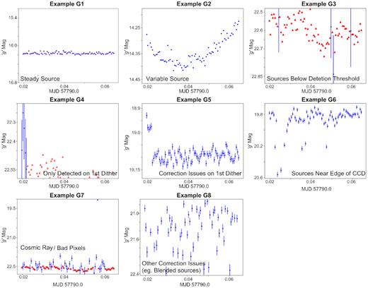
Antlia field examples of typical light curves present in each of the sub-groupings. The blue points represent source detections, the red triangles represent the limiting magnitudes of the exposures and are only present in the light curves when sources are not detected.
From the sub-grouping of clusters, we are able to meaningfully quantify the light curves for this field: finding that 93.5|${{\ \rm per\ cent}}$| are grouped into one cluster, of steady light curves, while ∼2.0|${{\ \rm per\ cent}}$| of light curves were affected by telescope dithering and/or the use of the hexapod on the DECam instrument, and 0.39|${{\ \rm per\ cent}}$| of light curves had photometric correction issues over the first five exposures (of the 80) due to the initial five point dither pattern and change in standard stars used for correction on certain CCDs.
5.2.2 Sub-groups identifying variable sources
The algorithm identified one cluster containing sources of true astrophysical variability, described in sub-grouping G2 in Table 3. These sources were cross-matched to several catalogues to check for known variability, as outlined in Section 5.1.2. In this group, we identified six variable sources, three of which have been previously catalogued and three sources discovered by this work. Source IDs, name, coordinates, known catalogue ID (if available), and period are shown in Table 4.
Sources identified showing variability in J04-55 and Antlia fields. Note: lines in bold indicate discoveries in this work.
| Field | DWF ID | Catalogued ID | Probable typea | Period (d)b |
|---|---|---|---|---|
| Antlia | DWF102919.102-355133.303 | SSS J102919.0-355133 | Spotted Star | 0.34 |
| Antlia | DWF102938.901-345415.969 | SSS J102938.8-345416 | W Ursae Majoris | 0.27 |
| Antlia | DWF103105.927-360744.003 | SSS J103105.8-360742 | W Ursae Majoris | 0.44 |
| Antlia | DWF102552.421-354418.436 | Discovered in this work | δ Scuti or γ Doradus | – |
| Antlia | DWF103240.961-344522.875 | Discovered in this work | – | – |
| Antlia | DWF103147.030-354553.653 | Discovered in this work | – | – |
aFor previously catalogued sources, type is identified by catalogue, if newly discovered source, type approximated from CMD position (see Appendix C1).
bFor previously catalogued sources the period is taken from the discovery survey, if newly discovered source period is not known.
cAbsolute G-Band magnitude as calculated using Gaia parallax information.
Of the three newly discovered sources in this sub-grouping, we are unable to unambiguously identify the variable types of two sources using the CMD in Appendix C1. The CMD location of the reamining source was calculated using Gaia data release 2 parallax and photometric information (Evans et al. 2018; Luri et al. 2018). The CMD position is overlaid on the variability CMDs presented in work by Gaia Collaboration (2019) and subsequently used for likely type identification in 3. We are unable to confidently classify DWF103240.961-344522.875 in the CMD because of its large Gaia parallax uncertainty and, thus, absolute magnitude. On the other hand, DWF103147.030-354553.653 sits in an area where few pulsating objects are found, between main sequence stars and white dwarfs but where cataclysmic variables are common. A source in this region was shown by Gaia Collaboration (2019) to be likely a cataclysmic variable (CV). The light curves for all six sources are presented in Fig. 5.
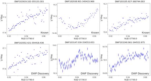
Three previously known and three newly discovered variable sources as identified in sub-group G2.
5.2.3 Variable/transient sources
A total of 2169 light curves were unclustered by HDBSCAN and not assigned to a specific cluster in our analysis of the Antlia field. These light curves can be seen to sit along the outskirts of the main grouping of G1 in Fig. 3, as well as occupying similar feature space to other identified clusters. It is these light curves which are of particular interest for rare transient and variable events, as we expect any unusual and unique light curves in comparison to the majority to be identified as noise via HDBSCAN.
Two independent approaches were used to evaluate the unclustered light curves. The first was manual inspection of all 2169 light curves and the second was anomaly detection and ranking using astronomaly. This dual approach was taken to comparatively quantify the successful extraction of interesting anomalous light curves using astronomaly’s inbuilt isolation forest anomaly ranking. Here, astronomaly was used to explore groupings of similar light curves through its inbuilt interactive t-SNE plot.
During our evaluation, sources within the unclustered grouping, were again cross-matched to VSX, DES, and the Catalina Surveys Southern Periodic Variable Star Catalogue, to identify previous detections and classifications. The majority of the unclustered light curves were false positives caused by dithering affects on sources. However, amongst the false positives we identify nine variable sources, six of which were previously catalogued by surveys, with the remaining three sources discovered in this work. We further discover an ultrafast flaring source, with positioning on the CMD suggesting the source is consistent with M dwarf flares. Optical flare events evolving on very short time-scales (seconds-to-minutes) such as this have previously only been identified using 10 s cadence of NUV GALAX data by Brasseur, Osten & Fleming (2019), uncovering a previously unexplored population of short duration of stellar flares. Source IDs, name, coordinates, known catalogue ID (if available) and period are shown in Table 5. The light curves for each of the sources are presented in Fig. 6. The newly discovered sources showing variability are overlaid on the CMD in Appendix C1 as purple triangles.
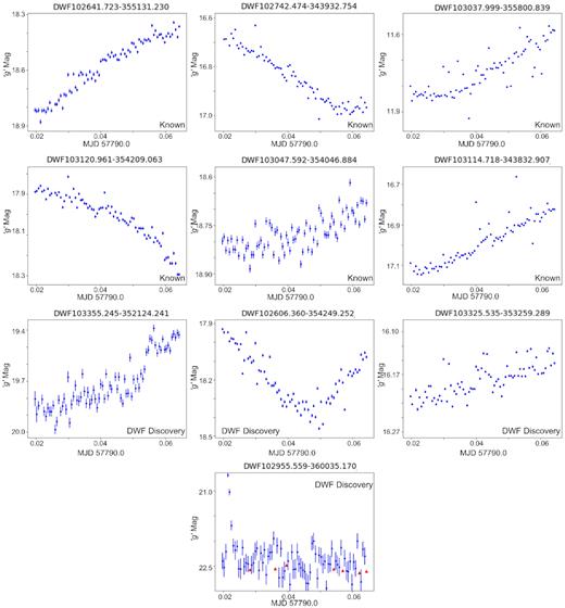
Size previously known and four newly discovered variable sources as identified in the grouping of unclustered light curves. The blue points represent source detections, while the red triangles represent the limiting magnitudes of the exposures and are only present in the light curves when sources are not detected.
Sources identified showing variability in J04-55 and Antlia fields. Note: lines in bold indicate discoveries in this work.
| Field | DWF ID | Catalogued ID | Typea | Period (d)b |
|---|---|---|---|---|
| Antlia | DWF102641.723-355131.230 | SSS J102641.7-355130 | W Ursae Majoris | 0.29 |
| Antlia | DWF102742.474-343932.754 | SSS J102742.4-343933 | W Ursae Majoris | 0.27 |
| Antlia | DWF103120.961-354209.063 | SSS J103120.8-3542094 | W Ursae Majoris | 0.27 |
| Antlia | DWF103037.999-355800.839 | ASAS J103038-3558.0 | β Persei | 0.72 |
| Antlia | DWF103047.592-354046.884 | SSS J103047.5-354047 | RR Lyrae | 0.31 |
| Antlia | DWF103114.718-343832.907 | SSS J103114.5-343834. | RR Lyrae | 0.33 |
| Antlia | DWF102606.360-354249.252 | Discovered in this work | UV Ceti or T Tauri | – |
| Antlia | DWF103355.245-352124.241 | Discovered in this work | T Tauri | – |
| Antlia | DWF103325.535-353259.289 | Discovered in this work | γ Doradus | – |
| Antlia | DWF102955.559-360035.170 | Discovered in this work | Ultrafast flare | – |
aFor previously catalogued sources, type is identified by catalogue, if newly discovered source, type approximated from CMD position (see Appendix C1).
bFor previously catalogued sources, the period is taken from the discovery survey, if newly discovered source period is not known.
cAbsolute G-Band magnitude as calculated using Gaia parallax information.
5.2.4 astronomaly performance
We utilized the large set of unclustered light curves identified in the Antlia field to test the abilities of astronomaly to present only the most astrophysically anomalous light curves to astronomers in a timely manner. astronomaly takes less than 2 min to process the features through the isolation forest algorithm and launch the interactive web GUI.
Using the astronomaly front end GUI to visually inspect each light curve in ranked order, we identified the nine variable sources within the top 280 of 2000 highest ranking anomalous light curves taken from the grouping of unclustered sources and the ultrafast flare event was identified within the first 600. By using both clustering and astronomaly we were able to find all the anomalies in the first 0.9 |${{\ \rm per\ cent}}$| of the over all Antlia data. This result highlights the possibility to significantly reduce the amount of time needed for light-curve evaluation of anomalous events by astronomers, and will be continued to be utilized in the future analysis of DWF light curves.
A more recent version of astronomaly contains human-in-the-loop learning, designed specifically to deal with finding objects that are swamped by more anomalous points (according to the machine learning) but are actually more mundane objects.
5.2.5 Validating the completeness for Antlia field
Similar to Section 5.1.3, we took several steps to verify all variable sources which were identified. Within a 1.5 degree radius of the field centre, 22 catalogued variable sources (with periods less than 1 d) existed in the VSX catalogue and within DECam’s CCD footprint. Nine of the known variable sources were recovered as anomalies in this work, both being identified in the cluster of variables and within the unclustered grouping of most anomalous light curves, as explained in detail in Sections 5.2.1 and 5.2.2. Of the remaining sources, six did not show significant variability over the ∼80 min period and were subsequently clustered in the grouping of steady light curves, consistent with their longer recorded periods (see Appendix D2 for full details). The remaining seven were either below detection threshold, at saturation limits, or photometrically affected by dithering and were clustered accordingly. astronomaly was used to display the top 2000 light curves (limited to 2000 light curves by astronomaly for the handling of the interactive t-SNE plot) ranked most anomalous via the isolated forest algorithm over the identified clusters. After visual inspection, no additional interesting light curves were found.
6 CONCLUSION
Existing and future astronomical surveys are continuously pushing the bounds of the known transient universe, and the ability to efficiently probe a large number of light curves in a timely manner will become vital in the exploration of regions of previously known and unknown classes of events. In this work, we have successfully shown the capability of unsupervised machine learning methods to rapidly and thoroughly explore fast cadenced data collected by transient surveys, using the DWF program as an example. By taking a two-step approach of both clustering and anomaly/outlier detection, we were able to identify seven previously unidentified variable stars. We also identified two classes of stellar flares, one classical flare and one rapidly evolving flare, further demonstrating the effectiveness of our unsupervised methods and the unique capability of the DWF program. Notable is the speed of which this method can be performed. Feature extraction takes ∼110 s per 1000 light curves and when run in parallel (on the OzSTAR supercomputer) can complete a set of 70 000 light curves in less than 15 min. The HDBSCAN clustering takes a further ∼2 min, and in total, a set of 70 000 light curves can be ready for human evaluation using astronomaly within 20 min. Both the speed and ease of use our method demonstrates the ability of unsupervised methods in meaningfully evaluating light curves to identify source variability. This method is well suited for the use on current and upcoming surveys for anomaly detection, for which hundreds of millions of light curves will inevitably be produced.
Finally, we stress that this work explores a small fraction of the full DWF data set, only two fields for 80–90 min each. Future work will involve the evaluation of 250+ h of data for 17 fields. Moreover, as DWF runs typically occur over six consecutive nights, additional variable sources will be found over a range of phase durations when the data is analysed over the full run duration for the two fields explored here. Furthermore, we plan to use this unsupervised method on light curves combined over multiple nights to search for long period variables, which would otherwise appear steady in single night light curves.
ACKNOWLEDGEMENTS
We would like to thank the organisers of the 2019 Kavli Summer Program in Astrophysics hosted at the University of California, Santa Cruz, without which this collaboration and work would not have been possible. We give thanks to our reviewer for their feedback, insight and comments. The program was funded by the Kavli Foundation, The National Science Foundation, UC Santa Cruz, and the Simons Foundation. Part of this research was funded by the Australian Research Council Centre of Excellence for Gravitational Wave Discovery (OzGrav), CE170100004. We acknowledge the financial assistance of the National Research Foundation (NRF). Opinions expressed and conclusions arrived at, are those of the authors and are not necessarily to be attributed to the NRF. This work was partly supported by the GROWTH (Global Relay of Observatories Watching Transients Happen) project funded by the National Science Foundation under PIRE Grant No 1545949. This work has made use of data from the European Space Agency (ESA) mission Gaia (https://www.cosmos.esa. int/gaia), processed by the Gaia Data Processing and Analysis Consortium (DPAC, https://www.cosmos.esa.int/web/gaia/dpac/consortium). Funding for the DPAC has been provided by national institutions, in particular the institutions participating in the Gaia Multilateral Agreement.
This project used data obtained with the Dark Energy Camera (DECam), which was constructed by the Dark Energy Survey (DES) collaboration. Funding for the DES Projects has been provided by the U.S. Department of Energy, the U.S. National Science Foundation, the Ministry of Science and Education of Spain, the Science and Technology Facilities Council of the United Kingdom, the Higher Education Funding Council for England, the National Center for Supercomputing Applications at the University of Illinois at Urbana-Champaign, the Kavli Institute of Cosmological Physics at the University of Chicago, the Center for Cosmology and Astro-Particle Physics at the Ohio State University, the Mitchell Institute for Fundamental Physics and Astronomy at Texas A&M University, Financiadora de Estudos e Projetos, Fundação Carlos Chagas Filho de Amparo à Pesquisa do Estado do Rio de Janeiro, Conselho Nacional de Desenvolvimento Científico e Tecnológico and the Ministério da Ciência, Tecnologia e Inovacão, the Deutsche Forschungsgemeinschaft, and the Collaborating Institutions in the Dark Energy Survey. The Collaborating Institutions are Argonne National Laboratory, the University of California at Santa Cruz, the University of Cambridge, Centro de Investigaciones Enérgeticas, Medioambientales y Tecnológicas-Madrid, the University of Chicago, University College London, the DES-Brazil Consortium, the University of Edinburgh, the Eidgenössische Technische Hochschule (ETH) Zürich, Fermi National Accelerator Laboratory, the University of Illinois at Urbana-Champaign, the Institut de Ciències de l’Espai (IEEC/CSIC), the Institut de Física d’Altes Energies, Lawrence Berkeley National Laboratory, the Ludwig-Maximilians Universität München and the associated Excellence Cluster Universe, the University of Michigan, the National Optical Astronomy Observatory, the University of Nottingham, the Ohio State University, the OzDES Membership Consortium the University of Pennsylvania, the University of Portsmouth, SLAC National Accelerator Laboratory, Stanford University, the University of Sussex, and Texas A&M University. Based on observations at Cerro Tololo Inter-American Observatory, National Optical Astronomy Observatory which is operated by the Association of Universities for Research in Astronomy (AURA) under a cooperative agreement with the National Science Foundation.
DATA AVAILABILITY
The data underlying this article will be shared on reasonable request to the corresponding author.
Footnotes
The hexapod mechanism is a set of six pneumatically driven pistons that actuate to precisely align the optical elements between exposures.
REFERENCES
APPENDIX A: FEATURES
Features used in this work and the properties of the light curves they represent.
| Feature | Description | Inputs | Refs |
|---|---|---|---|
| Amplitudes | Half the difference between | Magnitude | Richards et al. (2011) |
| the median of the maximum 5 percent and the median | |||
| of the minimum 5 percent magnitude. | |||
| Autocorrelation length | Length of linear dependence of a signal with | Magnitude | Kim et al. (2011) |
| itself at two points in time | |||
| Beyond1Std | Percentage of points beyond one | Magnitude |$\&$| Error | Richards et al. (2011) |
| standard deviation from the weighted mean | |||
| CARmean | The mean of a continuous time autoregressive | Magnitude, Time |$\&$| Error | Pichara et al. (2012) |
| model using a stochastic differential equation | |||
| CARσ | The variability of the time series on | Magnitude, Time |$\&$| Error | Pichara et al. (2012) |
| time-scales shorter than τ | |||
| CARτ | The variability amplitude of the | Magnitude, Time |$\&$| Error | Pichara et al. (2012) |
| time series | |||
| H1 | Amplitude derived using the Fourier | Magnitude | Kim & Bailer-Jones (2016) |
| decomposition | |||
| Con | The number of three consecutive | Magnitude | Kim et al. (2011) |
| data points that are brighter or fainter then 2σ | |||
| and normalized by N −2 | |||
| Linear trend | Slope of a linear fit to the light curve | Magnitude |$\&$| Time | Richards et al. (2011) |
| MaxSlope | Maximum absolute magnitude slope between two | Magnitude |$\&$| Time | Richards et al. (2011) |
| consecutive observations | |||
| Mean | The mean magnitude | Magnitude | Kim et al. (2014) |
| Mean variance | the ratio of the standard deviation | Magnitude | Kim et al. (2011) |
| to the mean magnitude | |||
| Median absolute deviation | The median discrepancy of the data | Magnitude | Richards et al. (2011) |
| from the median data | |||
| Median buffer range percentage | Fraction of photometric points | Magnitude | Richards et al. (2011) |
| with amplitude/10 of the median magnitude | |||
| Pair slope trend | The fraction of increasing first differences | Magnitude | Richards et al. (2011) |
| minus the fraction of decreasing | |||
| first differences | |||
| Q31 | The difference between the 3rd | Magnitude | Kim et al. (2014) |
| and 1st quarterlies | |||
| R21 | 2nd to 1st amplitude ratio derived | Magnitude | Kim & Bailer-Jones (2016) |
| Using the Fourier decomposition | |||
| R31 | 3rd to 1st amplitude ratio derived | Magnitude | Kim & Bailer-Jones (2016) |
| using the Fourier decomposition | |||
| Rcs | Range of cumulative sum | Magnitude | Richards et al. (2011) |
| Skew | The skewness of the sample | Magnitude | Richards et al. (2011) |
| Slotted autocorrelation | Slotted autocorrelation length | Magnitude |$\&$| Time | Protopapas et al. (2015) |
| Function length | |||
| Small Kurtosis | Small sample Kurtosis of magnitudes | Magnitude | Richards et al. (2011) |
| Standard deviation | Standard deviation of the magnitudes | Magnitude | Richards et al. (2011) |
| StetsonKAC | Stetson K applied to the slotted | Magnitude | Stetson (1996), Kim et al. (2011) |
| autocorrelation function of the light curve | |||
| Variability index | Ratio of the mean of the square of successive differences | Magntiude | Kim et al. (2011) |
| to the variance of data points |
APPENDIX B: astronomaly WEB INTERFACE
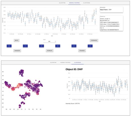
Top) astronomaly web interface ‘Anomaly Scoring’ tab, where light curves can be visually assessed in order of anomaly ranking as determined by the isolation forest algorithm. Bottom) astronomaly web interface ‘Clustering’ tab, displaying an interactive t-SNE plot produced from the input data. The points within the t-SNE can be clicked and then the corresponding light curve will be displayed to the right of the screen. This feature is extremely useful for searching similar light curves based on their features.
APPENDIX C: COLOUR MAGNITUDE PLOT – NEWLY DISCOVERED TRANSIENTS/VARIABLES FROM THIS WORK
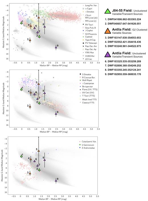
Known pulsating (top panel), eruptive (centre panel), and cataclysmic (bottom panel) variables are shown on the CMDs taken from the Gaia Collaboration (2019), with the newly discovered variable and flaring sources (large symbols) overlaid. The green triangles represented sources found in the J04-55 field, the orange represent newly discovered sources from G2 in the Antlia field, and the purple represent the newly discovered sources, which HDBSCAN was not able to cluster. Schlafly & Finkbeiner (2011) was used to correct Gaia BP-RP for galactic reddening.
APPENDIX D: PREVIOUSLY CATALOGUED SOURCES
Variable star index (VSX) catalogued variable sources within the DWF J04-55.
| Field | Catalogue name | Type | Period (d) | Notes |
|---|---|---|---|---|
| DWF J04-55 | SSS J041109.9-544851 | W Ursae Majoris eclipsing binary | 0.31 | Identified in this work as anomalous |
| DWF J04-55 | ASAS J040958-5520.2 | Cepheid | 9.20 | Below detection threshold most exposures |
| DWF J04-55 | ASAS J041436-5441.9 | Contact binary | 0.45 | Identified in this work as anomalous |
| DWF J04-55 | ASASSN-V J040807.97-541827.2 | W Ursae Majoris eclipsing binary | 0.55 | Identified in this work as anomalous |
| DWF J04-55 | ASASSN-V J040449.48-552715.9 | W Ursae Majoris eclipsing binary | 0.27 | Identified in this work as anomalous |
| DWF J04-55 | SSS J041229.7-543444 | Asymmetric RR Lyrae | 0.55 | Below detection threshold most exposures |
| DWF J04-55 | SSS J040348.1-552845 | W Ursae Majoris eclipsing binary | 0.39 | Below detection threshold most exposures |
| DWF J04-55 | SSS J040421.3-551639 | β Persei eclipsing binary | 1.15 | Flat light curve, unchanging over observations |
| DWF J04-55 | ASAS J040237-5502.5 | Detached eclipsing binary | 1.93 | Flat light curve, unchanging over observations |
| DWF J04-55 | WISE J041127.4-543854 | β Persei eclipsing binary | 0.68 | Flat light curve, unchanging over observations |
| DWF J04-55 | ASASSN-V J041337.83-554819.5 | Variable star of unspecified type | unknown | Flat light curve, unchanging over observations |
| DWF J04-55 | ASASSN-V J040350.67-545214.6 | Spotted stars that weren’t | 0.49 | Flat light curve, unchanging over observations |
| classified into a particular class |
Variable star index (VSX) catalogued variable sources within the DWF Antlia field.
| Field | Catalogue Name | Type | Period (d) | Notes |
|---|---|---|---|---|
| DWF Antlia | SSS J103047.5-354047 | RR Lyrae | 0.31 | Identified in this work as anomalous |
| DWF Antlia | SSS J102938.8-345416 | W Ursae Majoris eclipsing binary | 0.27 | Identified in this work as anomalous |
| DWF Antlia | SSS J103120.8-354209 | W Ursae Majoris eclipsing binary | 0.27 | Identified in this work as anomalous |
| DWF Antlia | ASAS J103038-3558.0 | β Persei-type eclipsing binary | 0.72 | Identified in this work as anomalous |
| DWF Antlia | SSS J103114.5-343834 | RR Lyrae | 0.33 | Identified in this work as anomalous |
| DWF Antlia | SSS J102742.4-343933 | W Ursae Majoris eclipsing binary | 0.27 | Identified in this work as anomalous |
| DWF Antlia | SSS J103105.8-360742 | W Ursae Majoris eclipsing binary | 0.44 | Identified in this work as anomalous |
| DWF Antlia | SSS J102641.7-355130 | W Ursae Majoris eclipsing binary | 0.29 | Identified in this work as anomalous |
| DWF Antlia | SSS J102919.0-355133 | Spotted stars that weren’t | 0.34 | Identified in this work as anomalous |
| classified into a particular class | ||||
| DWF Antlia | SSS J102615.2-351023 | RR Lyrae | 0.50 | Below detection threshold most exposures |
| DWF Antlia | SSS 110101:103109-350150 | Dwarf novae | unknown | Flat light curve, unchanging over observation |
| DWF Antlia | SSS J102933.7-354152 | W Ursae Majoris eclipsing binary | 0.29 | Flat light curve, unchanging over observation |
| DWF Antlia | SSS J103200.4-353401 | W Ursae Majoris eclipsing binary | 0.44 | Flat light curve, unchanging over observation |
| DWF Antlia | SSS J102734.7-353154 | W Ursae Majoris eclipsing binary | 0.40 | Flat light curve, unchanging over observation |
| DWF Antlia | SSS J102717.6-353645 | β Persei-type eclipsing binary | 0.89 | Flat light curve, unchanging over observation |
| DWF Antlia | SSS J103425.0-350405 | W Ursae Majoris eclipsing binary | 0.41 | Flat light curve, unchanging over observation |
| DWF Antlia | SSS J102712.4-353219 | RR Lyrae | 0.63 | At saturation limit with photometry affected, |
| DWF Antlia | SSS J103237.3-345913 | Spotted stars that weren’t | 0.30 | At saturation limit with photometry affected, |
| classified into a particular class | ||||
| DWF Antlia | SSS J103436.8-352812 | W Ursae Majoris eclipsing binary | 0.35 | At saturation limit with photometry affected |
| DWF Antlia | SSS J103157.1-351718 | W Ursae Majoris eclipsing binary | 0.32 | Light curve photometricly affected. |
| DWF Antlia | SSS J103440.2-351511 | W Ursae Majoris eclipsing binary | 0.31 | Affected photometry from CCD edge |
| identified as such in G6. | ||||
| DWF Antlia | SSS J102906.8-360355 | W Ursae Majoris eclipsing binary | 0.32 | Affected photometry from CCD edge, |
| identified as such in G6. |
APPENDIX E: LIGHT-CURVE TRAITS
Clusters identified from Antlia field light curves using HDBSCAN.
| Cluster | Number of | Notes |
|---|---|---|
| light | ||
| unclustered | 2169 | Light curves with majority non-detections as well as possible variable sources and photometry affected by telescope dithering. |
| 0 | 6 | Only detected on five point dithers, either beginning, middle or end of observations. |
| 1 | 6 | Variable sources. |
| 2 | 20 | Sources near edge of ccd resulting in dimming and brightening as the source moves ccd position during observations. |
| 3 | 30 | Only detected on five point dithers, either beginning, middle or end of observations. |
| 4 | 23 | Only detected on five point dithers, either beginning, middle or end of observations. |
| 5 | 7 | First five point dither detections correction issues of 0.1–0.2 mag. |
| 6 | 19 | First five point dither detections correction issues of 0.1–0.2 mag. |
| 7 | 58 | First five point dither detections correction issues of 0.1–0.2 mag. |
| 8 | 16 | Bright Sources on ccd extension 30, Issues with correction over the night. |
| 9 | 10 | First five point dither detections correction issues of 0.1–0.2 mag. |
| 10 | 17 | First five point dither detections correction issues of 0.1–0.2 mag. |
| 11 | 107 | First five point dither detections correction issues of 0.1–0.2 mag. |
| 12 | 23 | One or more detections affected by Cosmic Rays, pixel faults, etc. |
| 13 | 5 | First five point dither detections correction issues of 0.1–0.2 mag. |
| 14 | 14 | Sources near edge of ccd resulting in dimming and brightening as the source moves ccd position during observations. |
| 15 | 11 | Bright Sources on ccd extension 30, issues with correction over the night. |
| 16 | 22 | Bright Sources on ccd extension 30, issues with correction over the night. |
| 17 | 23 | Sources near edge of ccd resulting in dimming and brightening as the source moves ccd position during observations. |
| 18 | 20 | First five point dither detections correction issues of 0.1–0.2 mag. |
| 19 | 8 | Sources on ccd extension 30, Issues with correction over the night. |
| 20 | 226 | One or more detections affected by cosmic rays, pixel faults, etc and faint sources at detection threshold. |
| 21 | 12 | Only detected on five point dithers, either beginning, middle or end of observations. |
| 22 | 6 | Only detected on five point dithers, either beginning, middle or end of observations. |
| 23 | 7 | Only detected on five point dithers, either beginning, middle or end of observations. |
| 24 | 12 | Sources near edge of ccd resulting in dimming and brightening as the source moves ccd position during observations. |
| 25 | 17 | Defuse or blended sources. |
| 26 | 156 | Sources near edge of ccd resulting in dimming and brightening as the source moves ccd position during observations. |
| 27 | 11 | Only detected on five point dithers, either beginning, middle or end of observations. |
| 28 | 11 | Only detected on five point dithers, either beginning, middle or end of observations. |
| 29 | 951 | Sources near edge of ccd resulting in dimming and brightening as the source moves ccd position during observations. |
| 30 | 19 | Faint sources behind defuse galaxies/ blended point sources |
| 31 | 5 | One or more detections affected by cosmic rays, pixel faults, etc. |
| 32 | 5 | Only detected on five point dithers, either beginning, middle or end of observations. |
| 33 | 12 | Faint sources at detection threshold. |
| 34 | 6 | Faint sources at detection threshold. |
| 35 | 5 | Faint sources at detection threshold. |
| 36 | 58 279 | Steady light curves. |
