


Abstract
Ensemble modelling is a quantitative method that combines information from multiple individual models and has shown great promise in statistical machine learning. Ensemble models have a theoretical claim to being models that make the ‘best’ predictions possible. Applications of ensemble models to health research have included applying ensemble models like the super learner and random forests to epidemiological prediction tasks. Recently, ensemble methods have been applied successfully in burden of disease estimation. This article aims to provide epidemiologists with a practical understanding of the mechanisms of an ensemble model and insight into constructing ensemble models that are grounded in the epidemiological dynamics of the prediction problem of interest. We summarize the history of ensemble models, present a user-friendly framework for conceptualizing and constructing ensemble models, walk the reader through a tutorial of applying the framework to an application in burden of disease estimation, and discuss further applications.
Ensemble models are a subset of machine learning with exciting applications in descriptive epidemiology.
Ensemble models can leverage epidemiological context and prior knowledge to make accurate and precise predictions.
Modern-day statistical and computational tools make ensemble models straightforward to implement for epidemiological research.
Background
A fundamental problem in descriptive epidemiology is ‘how many?’ For a deadly disease like malaria, how many people are dying of it, where and at what age? Is that better or worse than last year? For a disease like depression that does not kill directly, but affects many people for a long period of time, the question is how many people are suffering from it? Estimates of these metrics by age, sex and location, as well as how they are changing over time are critical data for public health decision-making.1,2
Globally, there are huge gaps in our knowledge about who is getting sick from what and who is dying, and there is a massive data integration challenge that can help to solve it. Although routine measurements are not available, it is also rare to know nothing. The challenge in answering the how many question is bringing together the sparse and noisy measurements that do exist to create estimates that take into account the biases and other limitations of these data.1,2
Machine learning methods (see glossary of terms in Table 1) have emerged as powerful tools in health research to tackle this data integration challenge and make predictions for important applications.3 Ensemble models are tools rooted in statistics and machine learning that have become known for making accurate, precise and computationally efficient predictions. Ensemble methods have been widely applied in health research, including in applying the super learner approach to create risk prediction scores4,5 and predict HIV-1 drug resistance,6 stacking survival models for breast cancer7 and predicting exposure-outcome dose-response curves8 (we direct readers to further explore ensemble models in the tutorial papers listed in the cited references4,8).
Glossary of terms
| Method | Description |
|---|---|
| Ensemble methods | A technique using multiple learning algorithms, or multiple statistical models, and combining them to improve estimates and predictive performance. |
| K-fold cross-validation | A technique for estimating predictive validity. Done by breaking the data into K groups and then dropping each one in succession for model training and creating out-of-sample predictions for it. The predictive validity metric is then estimated using the out-of-sample predictions. |
| Machine learning | Algorithms that aim to ‘learn’ or predict outputs from inputs (covariates) based on a dataset that contains both inputs and labelled output. |
| Out-of-sample predictions | Predictions from a model that are made for data that was not used in training the model. |
| Predictive validity metric | A metric used to assess the performance of a model’s predictions. |
| Random forest | Also known as random decision trees, an ensemble method for classification or regression that creates decision trees during training/learning to map an input to an output. |
| Root-mean-squared-error | A commonly used predictive validity metric, calculated as the square root of the average of the squared error in predictions compared with the observed data. |
| Super-learning (stacking) | An algorithm that finds the optimal combination of a number of prediction algorithms. |
The ensemble methodology has been adopted by scientists as a reliable way to answer descriptive epidemiological questions where we have noisy and often sparse data. In this paper, we focus on a subset of specific examples where ensemble models make use of this noisy and sparse data to make predictions for burden of disease estimation, a subset of descriptive epidemiology. We first develop a general framework for constructing ensemble models for descriptive epidemiology applications. In our main application, Foreman and colleagues developed an ensemble model called the Cause of Death Ensemble Model (CODEm) to make cause-age-sex-specific mortality predictions for every country from 1980 to the present-day using diverse and disparate data sources from all around the world as part of the Global Burden of Disease Study (GBD).9 These ensembles consist of many linear models with smoothing over space, time and age that use factors related to specific causes of death as the predicting variables. In two additional applications, we discuss the use of ensemble models to predict population-level distributions of risk factors using ensembles of probability density functions,10 and the use of ensembles to produce disease maps at the 5x5 km level with stacking of multiple generalized linear models.11–13
The ensemble modelling methodology
A brief history of the ensemble approach
Ensemble models are composed of statistical learning methods that are run on the data to predict some target parameter (e.g. mortality rate), with predictions then combined in some way over these different methods. The first theory behind the ensemble methodology was introduced in the early 1990s with what Wolpert called stacked generalization, referred to here as stacking.14 Cross-validation procedures had existed previously as a way to select the best-performing model out of a set of models based on some predictive validity metric, like root-mean-squared-error (RMSE). Wolpert proposed a method that could take information from all of the models and combine their predictions, rather than just using the predictions from the best one. Wolpert showed that this would out-perform naive methods that only used predictions from one model.14 Building on this general framework, Breiman developed an extension of stacking that used linear regression to combine the predictions made by each of the individual models.15 Because linear regression minimizes squared error, Breiman’s method of stacked regressions implicitly optimizes squared error predictive validity metrics in combining the predictions of individual models.15
Stacking and stacked regression were applied for a variety of prediction problems and studied theoretically for a better understanding of why combining predictions from multiple models works.16 Stacking was further generalized as the super learner, an ensemble of multiple algorithms, and explored theoretically by van der Laan and colleagues. They showed that the super learner was as asymptotically efficient as if one knew a priori the optimal model to use.17–20 Subsequent work even explored creating an ensemble of ensemble models.21 As modern statistical and computing methods have made the creation of ensemble models more tractable, ensemble modelling has gained popularity as repeatedly succeeding in making better predictions by combining the predictions of many different algorithms. In 2006, Netflix, the movie and TV streaming service, initiated a competition where teams could submit a model to make the best predictions for Netflix customers’ streaming preferences. All of the successful teams used some type of ensemble method.22
Why do ensemble models work?
The statistical theory underlying the superior performance of ensemble methods has been outlined in detail by others.16,17,19 Heuristically, we live in a complex world and deal with complex problems. In general, teams that are more ‘cognitively diverse’ are better at problem solving.23 A systematic analysis of studies on diversity in the workplace showed that most studies on organizational diversity found that teams that are more diverse in terms of roles and team functions have better performance.24 Diversity leads to improved performance when ideas are debated within the team, and when there is a culture of learning and synthesizing information.24 This is the philosophical underpinning of ensemble models: each component model brings a unique set of predictions. Performance is enhanced when model validation techniques ‘learn’ from all of the component models and ‘debate’ the best combination of them.
When do ensemble models work?
Statistical modelling tasks generally fall into two categories: inferential statistics and descriptive statistics. Questions like, ‘Does smoking cause lung cancer?’ are answered using causal modelling strategies that fall into the inferential category. Questions like ‘How many children are dying from malnutrition?’ or ‘How many children will die from malnutrition from now until 2040?’ are fundamentally descriptive. This is the application where ensemble models become very useful. Ensemble models require additional care when used in causal modelling. Other authors explore the rich intersection of prediction, machine learning and causal modelling in detail.25,26
An ensemble framework for descriptive epidemiology
Though there are many types of ensemble models, they all share a few key ingredients. We now present a framework for thinking about ensemble modelling that references and builds on methodology from stacked generalization and the super learner that we have just discussed,19,20 and relates to ensemble taxonomies developed by others27,28 but focuses particularly on breaking down the concepts and steps as they relate to descriptive epidemiology.
Labelled data and the prediction task
In burden of disease estimation, each location unit has a set of variables that may relate to the health status of the individuals living in that location, along with a set of health outcomes. In epidemiology, each individual in a cohort study has information on their exposure and outcome variables clearly defined and recorded at each time point. These are examples of labelled data: predictor and response variables with meaningful values for the prediction task at hand.
Once we have these labelled data, the prediction problem must be clearly defined. We use information from the labelled data to make predictions about the outcome(s) of interest, for the population of interest. Not only do we want to make predictions for data where we have the labels on the predictor variables but not the outcome variables, but also to make the best predictions we can for fully labelled data when we know that the data are noisy (e.g. when the outcome variable is measured poorly, we may be able to better predict it than just relying on the mismeasured variable we are provided with, and/or to narrow the uncertainty around the estimates). In our burden of disease example, we may want to use country-level variables on socio-economic status, fertility and vaccination coverage rates over time to predict child mortality from vaccine-preventable diseases over the next 10 years. In our epidemiology example, we might want to use observed relationships between exposure and outcome variables in a clinical trial as well as individual-level characteristics to predict which medication an individual will respond best to.
Component models
After defining the prediction problem that we want to solve, we can specify a set of what we will call component models, each of which will make its own predictions. In order to create an ensemble model, we must have a minimum of two distinct component models. Depending on the type of variables that we have, and the type of prediction task that we want to perform, a component model could take many different forms. Any two component models could be different in terms of functional forms (e.g. regressions that use ordinary least squares compared to a decision tree), or they could be very similar (e.g. two linear regression models that differ only in the inclusion or exclusion of a particular predictor). This flexibility in component model specification makes ensemble models attractive for a wide variety of prediction problems.
Estimate of prediction quality
There are two key elements to evaluating the quality of component model predictions: (i) a clearly defined metric representing prediction quality, and (ii) a method for estimating this metric. Examples of metrics of prediction quality are RMSE, median absolute deviation, Kullback-Leibler divergence29 and the Kolmogorov-Smirnov (KS) statistic.30
One can then estimate this metric in a variety of ways, some of which may give more robust estimates. An important consideration when choosing how to estimate the metric is that ultimately our goal is to make the best out-of-sample predictions. Another way of talking about the distinction between in- and out-of-sample predictions is having a training data set (in-sample) that is used to train the component model, and a test data set (out-of-sample) that is used solely for evaluating the performance of the component model. Methods of calculating performance measures that utilize this train-test framework are preferred when fitting flexible models to large datasets, because they help us avoid over-fitting the component model. Over-fitting is when a model is fit too closely to the training dataset. As a result, the model does not capture the signal between predictors and an outcome and instead fits to noise in the training data.
A common strategy for estimating predictive validity metrics is -fold cross-validation. This type of cross-validation strategy involves ‘hiding’ some data from the model and only training it on the data that are not hidden. After the model is trained, it makes predictions for the data points that were hidden using only the values of the predictor variables for the hidden outcomes, called out-of-sample predictions. We can then compare the predictions for the ‘hidden’ outcome to the observed outcome variable. We can repeat this process times so that eventually all of the data has been ‘hidden’ at some point. This will give us a robust estimate of the accuracy of out-of-sample predictions.31 Cross-validation is a very important feature of ensemble models in burden of disease estimation because we are often modelling with sparse data and thus are especially susceptible to over-fitting. Another strategy for estimating predictive validity metrics is to repeatedly hide data based on group labels (e.g. the data from locations are hidden).31 The strategy that works best for estimating the metric of predictive validity may differ based on the prediction problem at hand. It is often desired to hide data in such a way that reflects the true patterns of missingness observed.9
Method for combining predictions
The final step in creating an ensemble is to combine the predictions from the component models in a way that maximizes the quality of the predictions. At its most general level, this step requires (i) translating the predictive validity quality measure into some other measure that represents how much weight a component model’s predictions are given in the ensemble, and (ii) combining the predictions in a way that utilizes the weights. Weighting schemes and methods to combine predictions will vary based on the prediction problem. We will talk more about specific examples of weighting schemes with the application to cause of death modelling, and when we discuss other examples of ensemble modelling.
Application of the ensemble framework to predicting causes of death
We will now walk through an application of the ensemble methodology from the GBD Study32 called the CODEm that was first introduced by Foreman et al. in 2012.9 Foreman et al. give details of CODEm methods elsewhere.9 Here we present a high-level overview of these methods and describe how they fit into the more general ensemble framework outlined above. Figure 1 presents a conceptual flowchart for applying the ensemble modelling framework to CODEm.
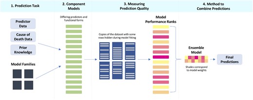
Conceptual flowchart applying the ensemble modelling framework to the Cause of Death Ensemble Model (CODEm).
Cause of death data and the prediction problem
Vital registration systems, verbal autopsies, disease registries and police reports are all examples of the diverse data sources that exist to record who is dying from what disease or injury.9,32 We do not always have cause of death data available for all locations and demographic groups across the world and through the years. Even for populations where we do, these data sources are often imperfect.
Component model specification
Additionally, the disease modeller might also be uncertain about which response variable to use. Different causes of death may also follow different data generating procedures and thus are better approximated by different types of models. She could predict the death rate, cause fraction or the death count.9 In the case where her cause of death has an abundance of data from many countries but lacks data in many others, she may also want to do more smoothing beyond the mixed-effect model.9
CODEm uses these different response variables and the modeller’s prior beliefs about which predictors are associated with her cause to create a set of component models that become the building blocks for the ensemble model. First, CODEm tests for significant relationships between different combinations of predictors and the cause-of-death outcome, resulting in component models with distinct combinations of predictors.9 Next, these component models are fit using a range of functional forms (predicting the logit-transformed cause fraction, the log-transformed death rate or the number of deaths per unit). Lastly, component models for diseases with lots of data may have better predictions and more robust uncertainty intervals after undergoing additional smoothing where predictions can borrow strength over the dimensions of age, space and time.9
Measuring prediction quality
To measure the quality of predictions from the component models, CODEm uses a combination of RMSE and trend (the percentage of predictions that correctly predict either the increasing or decreasing time-trend seen in the raw data). Now, how can we adequately capture the performance of the component models in the absence of data? We could randomly remove some of the data multiple times with a strategy like K-fold cross-validation. Or we could remove groups of locations at a time with a strategy like leave P-groups out. However, since cause of death data is based mainly on vital registration, disease-specific registries and verbal autopsy, we often find unique patterns of missingness in the data. CODEm has a custom cross-validation process, where it looks for real patterns of missingness in a given location and then replicates that pattern of missingness in other locations.9 We can do this many times so that we have multiple training-test sets that have patterns of missingness that look like the full data set. This is the method that CODEm uses to calculate the measure of quality based on RMSE and trend.9
This out-of-sample cross-validation strategy allows us to create ensemble models that are robust to missingness in the data. However, one must always be careful not to extrapolate beyond the range of the data. For example, if we have data for only 1980–2017, we would need more sophisticated statistical methods to predict into years that are not represented by the data.
Combining predictions to maximize quality
This may give a sensible point estimate, but we want to incorporate uncertainty from the model variability. Instead, CODEm sets a desired number of ‘draws’, (usually chosen to be 1000), and then takes number of draws from component model .9 The method of creating a draw from a component model means taking one sample from the variance-covariance matrix of the fixed effects estimates, multiplying that by the design matrix and adding on a random draw from the random effect probability distribution for the group that each data point belongs to. We typically report the mean of all 1000 draws as the best estimate of the prediction, and quantify uncertainty with an interval estimate ranging from the 2.5th and 97.5th percentiles of the 1000 draws.9 This strategy for estimating uncertainty can be used for any ensemble model that creates draws, or random realizations, from the component models. Figure 2 shows the ensemble model predictions using different values of ψ to weight the component models, and compares these models to the best component model.
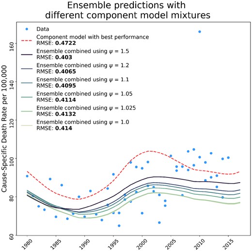
Influence of ψ values of ensemble composition and performance compared to the bestcomponent model. The figure shows the effect that the ψ weighting parameter has on the composition of the ensemble model, and how the RMSE for ensembles created with different weighting parameters compares to the best single component model included in the ensemble. The RMSE shown is calculated over all time series data and predictions included in the model, but we only show one time series to illustrate the performance of the ensemble.
Simple ensemble examples
To demonstrate some advantages of ensemble modelling, we have constructed simplified examples of the CODEm ensemble models for cause of death data in the USA. We have made an interactive example of this section available in a Jupyter Notebook on GitHub33 to clearly show the utility and accessibility of the ensemble framework. In these ensembles, we focus on varying one property of the component models: the independent variables included in each model. Additionally, instead of using RMSE and trend as the measure of prediction quality, we use only RMSE.
Further applications and discussion
Ensemble modelling in burden of disease estimation, let alone descriptive epidemiology, is not limited to the above application. Stacking in geostatistical models and risk factor density ensembles are two other prominent examples. To illustrate the flexibility of the ensemble approach to various epidemiological questions, we will briefly describe how these two applications fit into the ensemble framework.
Creating 5x5 km disease maps
This section outlines the approach of geostatistical stacking, with detailed methodology and applications elsewhere.11–13
Labelled data and the prediction problem
To predict disease at a more granular level, one can create maps of the probability of disease at the 5x5 km grid spanning any location of interest. The data used for geostatistical analyses are geographically located cases (e.g. case of malaria) aggregated up to this grid-level structure and paired with predictor variables.12,13
Component models
With more granularity, disease maps become complex and may not be well represented by a single model. The ‘stacking’ ensemble framework can account for this complexity11–13 Component models that tend to work well for this application include a generalized additive model with non-linear splines, a boosted regression trees model and a penalized regression (such as the lasso).11,12 Each of these popular models for high-dimensional data is used individually to predict the probability of disease at the 5x5 km level.
Measure of prediction quality
In order to assess out-of-sample performance, the data is split using 5-fold cross-validation holding out 20% of the data for testing each time. Each component model is fit on each of the five training sets and makes predictions for the five test sets. This process creates an out-of-sample prediction for the entire data set for each of the component models.11,12
Method of combining predictions
Rather than explicitly using RMSE or another metric to rank and then weight the models, the stacking method uses these out-of-sample predictions from each of the component models as independent variables in a linear regression model with priors specifying spatio-temporal correlation and a constraint that the coefficients for each model sum to 1. With this constraint, the coefficients act as weights on the component models, such that the ensemble is a weighted prediction where the weight on a given component model is determined based on its ability to predict the data points relative to the other component models. To make the final predictions, the in-sample predictions from the first stage are used as predictors in the second stage model that was fit using the out-of-sample predictions. Using in-sample predictions in this step allows us to be as precise as possible, while not over-fitting.11
Predicting distributions of risk factors
This section outlines the method of using ensembles to estimate probability density functions of random variables, with detailed methodology and application elsewhere.10
Labelled data and the prediction problem
Many variables that are considered risk factors for disease are continuous measures like weight, number of cigarettes smoked per day or lead exposure in blood. These types of variables are often measured in individual or household surveys. In order to make statements about population-level exposure to risk, it is necessary to predict the distribution function of the continuous risk variable.10
Component models
Since the functional form of the distribution is unknown, a set of continuous distribution functions could be specified, such as the normal distribution, log-normal, Weibull, logistic, etc. These functions act as component models that are fit to the mean and standard deviation of the individual-level data using the method of moments.10
Measure of prediction quality
The prediction of each component model is just the distribution function. The KS-statistic, which describes how close the predicted distribution function is to the empirical distribution function, can be used to measure each component model’s quality of prediction.10
Method of combining predictions
The ensemble distribution is a weighted linear combination of each of the component distributions, where the weights on the component models are the combination that minimizes the KS-statistic of the ensemble distribution (using Nelder-Mead numeric optimization).10
Discussion
Ensemble models are powerful tools that can be used to generate the most accurate predictions from incomplete and imperfect data. The flexibility of the ensemble modelling technique, as demonstrated in the applications of the ensemble modelling framework to three very different epidemiological applications—cause of death modelling, geospatial disease mapping and risk distribution modelling—makes it a useful tool for a variety of descriptive epidemiology problems in burden of disease estimation. Ensemble models use a range of ‘perspectives’, in the form of component models, and consequently perform better than single models can do by themselves. As seen in all three examples above, we make use of out-of-sample cross-validation to prioritize the best-performing component models to make the optimal final ensemble predictions.
In the field of burden of disease estimation where there are many unanswered questions about who is dying or suffering from what and where, ensemble models provide an analytic methodology that utilizes many sources of information in a smart way to answer these questions, filling a critical need for accurate health evidence. One can imagine exciting future applications for ensemble models in descriptive epidemiology. For example, non-fatal disease modelling (incidence and prevalence), disease burden forecasting and costing.
Acknowledgements
We would like to thank Aaron Osgood-Zimmerman and Kelly Cercy at IHME for providing supporting information for the additional applications of ensemble modelling to burden of disease estimation, and Drs Emmanuela Gakidou, Tony Blakely, Sherri Rose and Rebecca Bentley for providing feedback on drafts.
Funding
This research received no specific grant from any funding agency in the public, commercial or not-for-profit sectors.
Conflict of interest: A.D.F. has recently consulted for Kaiser Permanente, Agathos, NORC, and Sanofi. M.S.B. and M.M. declare no conflict of interest.

