Lower Danube Water Quality Quantified through WQI and Multivariate Analysis

Abstract

The aim of the present paper is to quantify water quality in the Lower Danube Region by using a series of multivariate techniques and the Water Quality Index (WQI). In this paper were measured 18 parameters upstream and downstream the city of Galati along the Danube River, namely: pH, Dissolved Oxygen (DO), Chemical Oxygen Demand (COD), Biochemical Oxygen Demand (BOD), N-NH₄⁺, N-NO₂⁻, N-NO₃⁻, N total, P-PO₄³⁻, SO₄²⁻, Cl⁻, Fe-total, Cr-total, Pb²⁺, Ni²⁺, Mn²⁺, Zn²⁺, As²⁺, in the interval winter 2013–winter 2016. The samples were either analyzed on the field, or sent for testing to the laboratory. The physicochemical parameters mentioned above were analyzed in accordance with the Romanian and International standards in force. The WQI was calculated according to Weighted Arithmetic Water Quality Index Method. The interdependencies between the selected physicochemical parameters were used for determining potential sources of pollution. Monitoring water quality dynamics in the period mentioned above favoured a series of relevant conclusions about the anthropic influence on water quality. Water quality was assessed by processing the measurements results, by calculating the water quality index (WQI), and by using the principal component analyses (PCA) and the response surface method (RSM) with the aim of correlating the indices for the physico-chemical parameters.

1. Introduction

Considering that water pollution and irrational water use represent two risk factors to the sustainable development of human society, constant monitoring of water quality is important. Natural and anthropogenic processes determine the chemical composition of the surface water [1,2].

The waters of the Danube are more or less affected by pollution with organic compounds, nutrients and heavy metals, pollutants from various sources such as industrial and domestic wastewaters, which are not treated sufficiently and rainwater which runs off the agricultural land where chemical fertilizers and pesticides are used. Monitoring water quality is important, especially since Romania is a member of the European Union (EU) and must comply with the specific legislation in the field (Water Framework Directive 2000).

The studied area (the confluence of the Danube River with two major rivers, the Siret and the Prut) is the largest hydrographic basin in the European Union. Due to the complexity of the aquatic ecosystems and to the existence of more pollution sources, there are no far-reaching studies in this area where pollution from 8 coastal countries is accumulated, the team which developed this study being the first to consider this area in the Danube basin [3,4,5,6]. The present study has been designed to continue past research on the region of the Lower Danube, the largest hydrographic basin in the European Union [2,7].

The importance of the study stems both from the sensitivity of aquatic ecosystems and from the fact that the Danube is the main source of drinking water for 1 million inhabitants in the Braila, Galati and Tulcea areas, the quality of surface waters having a direct impact on human health [2,7].

The quality of the surface water may be assessed by monitoring a series of physical and chemical parameters and by making a complex statistical analysis of the results obtained. Statistical analyses are made in order to simplify the complex sets of data obtained and to identify the most relevant set of parameters [2,7]. Establishing possible interdependencies between the parameters analyzed is important because once the main sources of pollution in a given period are identified, the existing problems may be solved and further risky situations may be prevented in case the water streams are exposed to long periods of flood and/or drought. The statistical analysis identifies the interdependencies established between two or more parameters which characterize the state of the system [8,9].

Rainfall, temperature, soil erosion and atmospheric conditions are some of the natural processes influencing the state of water systems, which should be taken into account when identifying possible interdependencies between the parameters analyzed. Pollution produced by domestic waters, industrial waters and agricultural activities are included in the category of anthropogenic processes. The impact of human and industrial activities may be quantified by analyzing the evolution of the ecosystems which suffer the actual impact [10,11]. It is important to use proper algorithms in order to include the most important parameters and their weight correctly.

This study was made by using set of classic statistic-mathematic methods. The different effects of the variables may not be interpreted independently, but only in close connection with the values of the other variables. There are no dependent or independent variables, and the multivariate analysis involves all the variables simultaneously and in the same proportion [12].

The interpretation of the variation in the physical and chemical parameters monitored and of the WQI was made by using the principal components analysis (PCA) and the response surface method (RSM).

In this study we used the Weighted Arithmetic Water Quality Index Method for determining the WQI. The studies taken into discussion in the present article started in 2010 and have been processed in time by using various methods, but the Weighted Arithmetic method has matched best the distribution of results, the complexity of the ecosystems and the quality categories in the legislation [2,6,7,13,14,15].

This method was selected because it allows the use of national standards which in turn, allow using the results and interpretations in surface water management in compliance with the national and EU legislation [2,7,13,14,15].

According to the EU legislation, the surface waters in Romania fall in the 2nd category (good water quality) and the use of this WQI calculation method allows researchers and specialists to use the values of the physico-chemical parameters specific to the 2nd quality waters of the standard WQI calculation [14,15]. In the EU Water Directive (WD) transposed in the national legislations of the Member States, surface water quality is classified in 5 categories regarding chemical quality: from “excellent” (category 1) to “very poor”’ (category 5) [15]. Danube water is included in categories 2 and 3. The WD includes categories which take into account each parameter separately and not the global quality index.

The use of statistical processing of the WQI physicochemical parameters through different methods leads to models, which follow the evolution of water quality according to the season in which the studies were conducted. Seasonal variations allow reference to a predictable model by means of which the rigorous management of the analyzed water course is ensured [10,11], and the results may be easily passed on to decision-makers responsible for water quality in Romania and at the EU level.

The main aim of this study is to define a suitable Water Quality Index for the Danube waters by taking into account the main chemical parameters and their weight. The means to reach this aim include: continuing studies on the quality of large aquatic ecosystems (Danube); targeting the weight ratios for the main pollutants by statistical processing (PCA, RSM); processing results over a significant period (4 years) for a system where seasonal variations are very important (for example, water flow variations from 1 to 2.2).

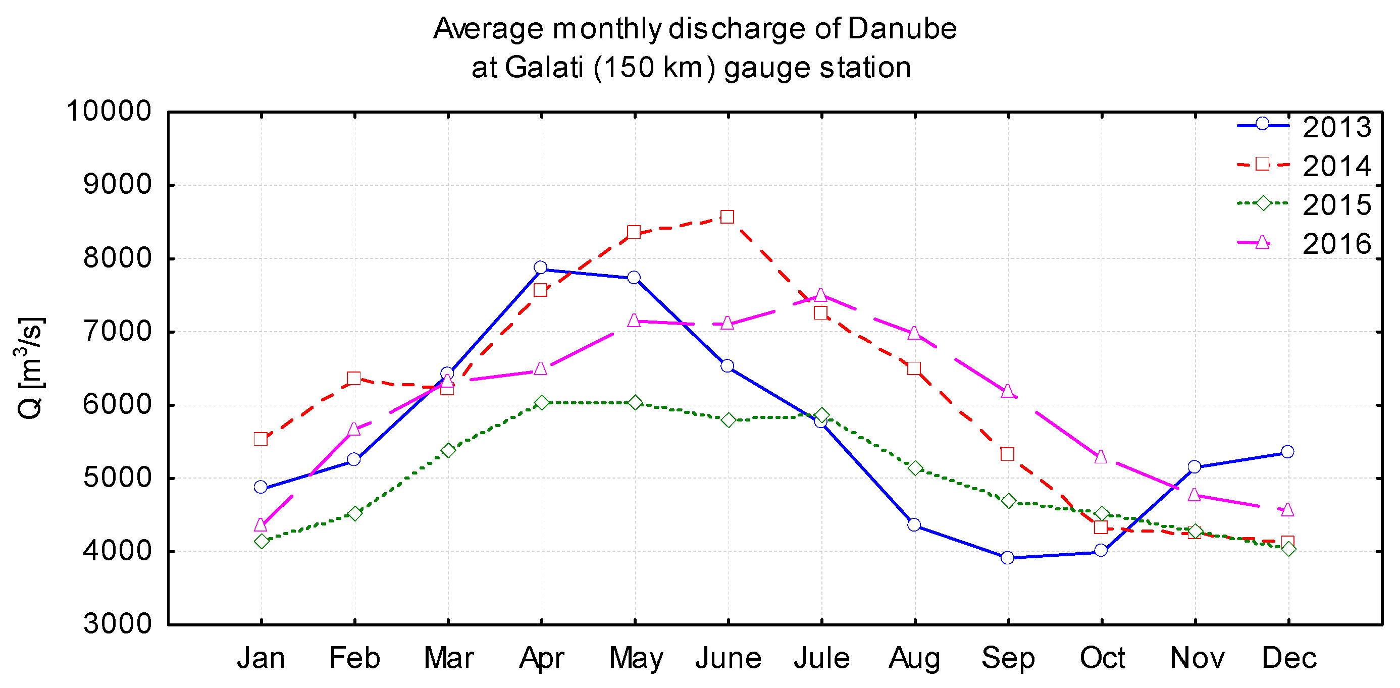
Water flow variation in Galati area during the measurements period was between 4000–8800 m³·s⁻¹. From a climatic point of view, the average annual temperature is around 10 °C. The average summer temperature is approx. 21 °C. In winter, north and northeast, cold air chambers produce temperature drops which fluctuate between 0.2 °C/−3 °C. The average monthly temperature is lower in January when reaches −3/−4 °C. During the year there are approximately 210 days with temperatures above 10 °C (National Meteorological Institute).

2. Materials and Methods

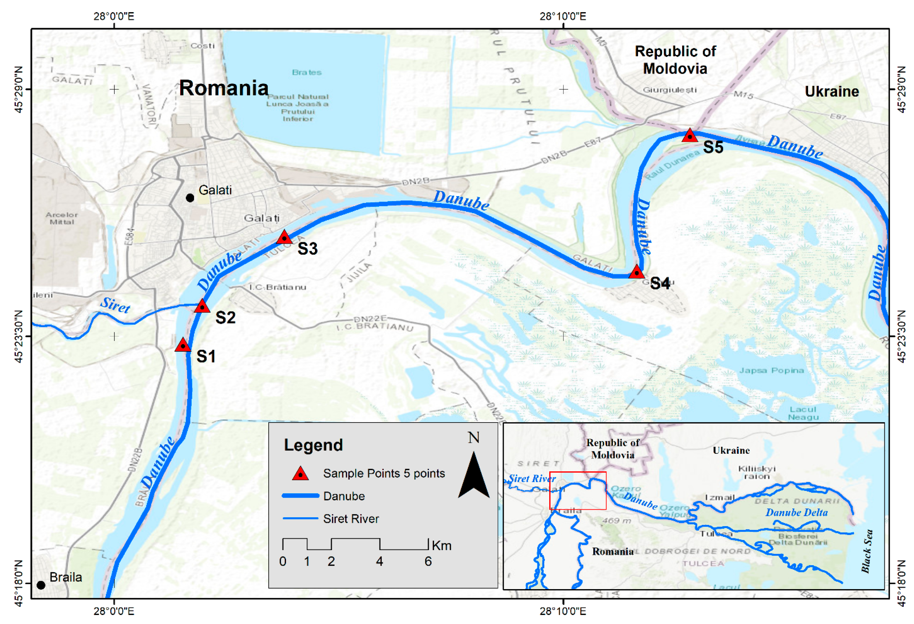
The assessment of the Danube water quality in the Galati County area implied monitoring 18 physical and chemical parameters, the water samples being collected from areas sensitively susceptible to anthropic influence: S1-Priza Dunarii (Sampling point 1-Series 1); S2-River Siret confluence (Sampling point 2-Series 2); S3-Ferry Crossing (Sampling point 3-Series 3); S4-River Prut confluence (Sampling point 4-Series 4); S5-Cotul Pisicii (Sampling point 5-Series 5) (Figure 1).

Sampling point S1 was located near the area where water is pumped for the drinking water supply of Galati.

Sampling point S2 was at the confluence of the Danube with an important river, the Siret. Due to its large flow, this river has an important contribution to the Danube water quality. Its water is charged with some pollutants coming from upstream (this river flows in an area in which the fertilizers and pesticides used in the intensive agricultural activities favour water load with nitrites, nitrates and phosphates), but also from the sewage treatment plant of one of Europe's largest steel mills.

Sampling point S3 was in the ferry crossing area where treated water coming from the municipal wastewater treatment plant is discharged.

Sampling point S4 was rather distant from the urban area.

Sampling point S5 was at the confluence of River Prut with the Danube. This river brings an important volume of water whose quality is inferior to that in the Danube. The Prut is a border river between Romania and the Republic of Moldova which flows through areas where intensive agriculture is practiced and where the industry is developed, the waste water from different communities in Republic of Moldavia being discharged without a proper treatment.

Apart from the location of the sampling points, it is of particular importance also the flow during the monitoring periods. Waterer flow variation in Galati area during the measurements period is presented in Figure 2.

The samples were taken and analyzed seasonally for a period of 4 years (between 2013 and 2016), once in spring (in March in all years), summer (in June in all years), autumn (in September in all years) and winter (in January in all years). The sampling was done in compliance with the standards in force. Polyethylene recipients were used and the samples were analyzed on the spot or they were sent to the testing laboratory (in the CREDENTIAL laboratory of the ECEE of “Dunarea de Jos” University of Galati) in the shortest time possible.

The tests were made observing the regulations in force. Sampling and sample analyses for physic-chemical parameters were made according the following Standard methods: SR EN 1899-2:2002 for BOD determination, SR EN ISO 6878:2005 for total phosphorus determination, SR SR EN ISO 11732:2005 for ammonium determination, ISO 15705:2002 for COD determination, SR EN 26777:2006 for nitrogen from nitrite determination, SR EN ISO 11905-1:2003 for nitrogen from nitrate determination, SR ISO 6332:1996/C91:2006—for iron total content, SR ISO 9297/2001—for chloride content, STAS 3069-87—for sulphate content, SR ISO 10566:2001—for lead content, SR ISO 9174-98—for Cr total. pH and OD were measured with a HANNA HI 9828 multiparameter analyzer. Spectrophotometric determinations were performed by using a Spectroquant NOVA 60 spectrophotometer and Merck kits. As²⁺ content was determined by spectrophotometric method with similar methods with standards-ASTM D2972-15 A; Zn²⁺ was determined photometrically in alkaline solution, zinc ions react with pyridylazoresorcinol (PAR); Ni²⁺ was determined photometrically oxidized by iodine [18,19,20,21,22,23,24,25,26,27,28,29,30].

All the quantification limits for the methods used in this paper are bellow the minimum values detected for all chemical species. All technical conditions for the quantification of chemical species (reliability, accuracy etc.) are met according to the standards in force (standards, regulations, etc.).

Pollutants are considered to be substances that are not naturally occurring in water or substances present in water in a higher concentration than the natural one.

The results obtained from the studies were interpreted by using different statistical methods.

The size of a given set of data which includes a large number of dependent variables is reduced by using the PCA method. In addition, this type of analysis allows for a better assessment of the correlations existing between the variables because it determines the involvement of individual chemical species in multiple influence factors1 [31,32,33,34].

The PCA analysis was used to verify the existence of a seasonal gradient in the set of physical and chemical data. The diagrams presented in this paper illustrate the grouping of parameters according to the way they influence each other.

The Response Surface Method (RSM) is a statistic empirical mathematical model, which allows creating a multidimensional regressive model on the basis of which the influence of the input variables on the output variable may be measured. The result may be represented either by a tridimensional graph, or by outline graphs, which illustrate the shape of the response surface. Outlines are constant response curves in the (xi, xj) plan and are obtained by maintaining all the other variables constant. A certain height of the response surface corresponds to each outline. This height indicates the degree to which the input variables influence the variable envisaged. The analysis implies successive stages of experimenting, modelling and data optimization [35,36].

The quality of a water stream is assessed by monitoring some of its physical, chemical and biological parameters, but also by calculating the water quality index. The WQI is a unique adimensional number which describes water quality at a certain moment and in a certain location [32,37,38] and which indicates any modification in the quality of the water [39,40]. Depending on the values obtained, a decision can be made regarding the possibility of considering the water potable, or of using it in industry or entertainment—related activities such as swimming, sports fishing and so on [2,41,42,43].

There are more ways of calculating the WQI, but the Weighted Arithmetic Water Quality Index Method [2,31,32,33,34,35] was used in our research because the relative weight of different variables was confirmed by the statistics studies [2,43,44,45,46,47,48,49].

Water quality index was determined by using the following equation:

$$WQI= \frac{{\displaystyle \sum }{W}_i{q}_i}{{\displaystyle \sum }{W}_i},$$

(1)

where WQI represents the water quality index. This parameter has values between 0 and 100 (it can exceed 100 if the area is heavily polluted); q_i represents a relative value of the water quality for each parameter, i represents the number of the parameters taken into consideration; W_i represents a factor which measures the importance of a given parameter in calculating the WQI (relative weight). q_i is calculated by using the following mathematical formula:

$$q_i=100\frac{V_i-V_0}{S_i-V_0},$$

(2)

where V_i represents the measured value (determined experimentally) of the i parameter; V₀ represents the ideal value of that parameter (it is 0 for all the parameters excepting the pH for which the value is 7 and the DO for whose value is 14.6 mg L⁻¹); S_i represents the standard value legally accepted for the water category in which the analysed water sample was included.

The Wi represents a factor which is calculated by using the following formula:

$$W_i = \frac{K}{S_i},$$

(3)

where K is a constant value calculated by the formula:

$$K=\frac{1}{{\displaystyle \sum }\left(\raisebox{1ex}{$1$}\!\left/ \!\raisebox{-1ex}{$S_i$}\right.\right)}$$

(4)

According to this method, the values of the WQI allow for a variation in the water quality from excellent (WQI = 0–25), to good (25–50), poor and very poor quality (51–75, 76–100) and very polluted (WQI > 100) [2,35]. The WQI was calculated by taking into consideration the Romanian standards for the surface waters [14].

3. Results and Discussion

Water quality is generally conditioned by a series of variables (parameters).

3.1. Variation of The WQI in The Sampling Points

The calculations made highlighted the fact that the WQI reached its maximum in sampling point S2 (the Siret confluence) in the spring of 2015. The values of the WQI in this point are the highest because there is more pollution on River Siret than on the Danube. This is due to the intake of nutrients which is easily noticeable during spring and summer when agriculture-related activities are intense, and to the intake originating in the city waste water which is purged by using mechanical processes and which is discharged in River Siret, not far from the confluence with the Danube. The values of the second quality water in this area sometimes exceed the maximal accepted values for COD, BOD, SO₄²⁻.

The highest values were recorded at all the sampling points during the spring of 2015, when the flow of the Danube water was at its lowest in the last 10 years. High values of the WQI were also recorded at the confluence of the Danube with River Prut. The lowest values were registered at sampling point S5 which is relatively far from direct entropic influences.

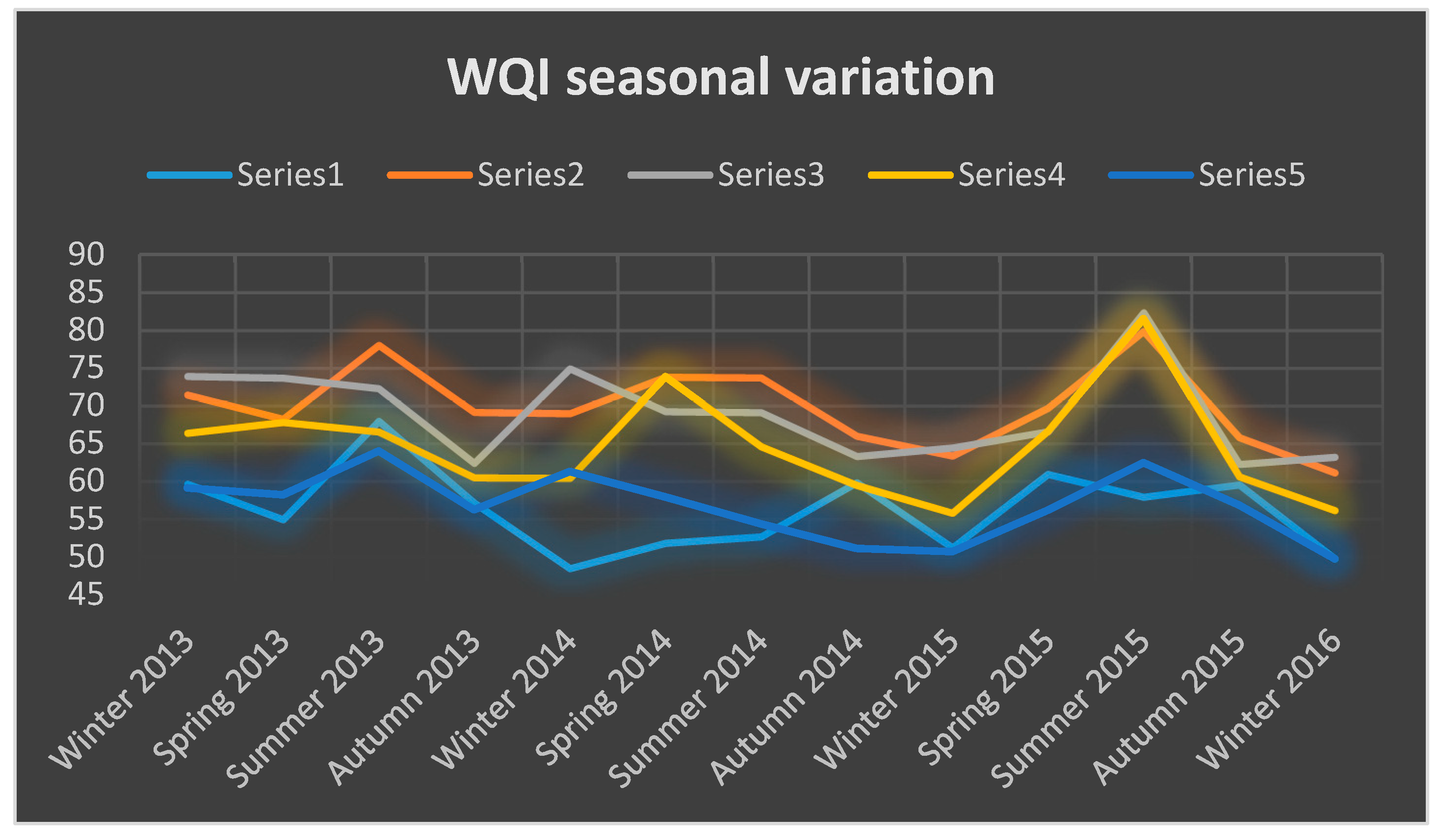
The highest values of the WQI were measured at sampling point S2 in all the seasons (Figure 3). This sampling point is at the confluence of the Danube with River Siret. The city wastewater, which is treated at SEAU Galati, and industrial wastewater, which is treated at SEAU of Arcellor Mettal Steel Factory, is discharged in River Siret, close to the confluence area. Analyzing the results obtained the fact may be noticed that the smaller values are recorded during winter when the values of the dissolved oxygen (DO) are high, and the values of COD, BOD and nutrients are small. It could be observed that COD values are influenced more by tributaries suggesting a more important load in organic species and mineral matter in reduced forms as well as the existence of anaerobic evolutions in sediments. COD values are important indicators for the efficiency of municipal wastewater treatment plant existent in the Galati–Braila area for a few years. In the calculation of the WQI, the nutrients have an important weight (W_i), and their presence in small quantities in winter leads, implicitly, to small values of these indices.

The highest values were recorded in the summer-autumn period, a possible explanation being the low flow of the water stream due to a period of drought.

Station S4 is rather distant from the urban area and, due to the phenomenon of self-purification, water quality in this area is superior to water quality in points S2, S3 and S5 and shows the impact of human activities on Danube water quality.

3.2. Statistical Analysis

In the first stage of the statistical analysis, the correlation coefficients of all the monitored parameters for each sampling point were evaluated. Correlations between the value series of the same parameter for neighbouring sampling points were also evaluated. Generally, there was a link between these datasets. The results will be presented in a future paper.

Additionally, primary statistical analyses were performed on the measured data series. The results are presented in a synthetic form in the

Table 1. Breakdown Table of Descriptive Statistics.

Variable	S1 Min Value	S1 Min Value	S1 Means ± Std.Dev	S2 Min Value	S2 Min Value	S2 Means ± Std.Dev.	S3 Min Value	S3 Min Value	S3 Means ± Std.Dev.	S4 Min Value	S4 Min Value	S4 Means ± Std.Dev.	S5 Min Value	S5 Min Value	S5 Means ± Std.Dev.
pH (upH)	7.82	8.82	8.30 ± 0.46	7.99	8.70	8.32 ± 0.33	7.82	8.36	8.14 ± 0.19	7.87	8.34	8.11 ± 0.15	7.82	8.28	8.14 ± 0.13
OD (mg·L−1)	4.78	12.00	5.65 ± 0.84	4.14	11.00	5.59 ± 1.34	4.73	9.00	5.84 ± 0.96	5.62	7.60	6.24 ± 0.52	5.12	9.00	6.56± 1.81
COD (mg·L−1)	5.5	35	19.30 ± 13.62	6.00	38.00	21.10 ± 13.79	5.7	34	16.66 ± 12.41	7.2	37	22.36 ± 11.25	6.1	26.0	15.20 ± 5.88
BOD (mg·L−1)	1.2	7.3	4.26 ± 2.70	2.10	8.30	4.63 ± 3.21	1.7	7.7	4.46 ± 2.89	1.7	6.7	4.10 ± 2.26	2.0	5.2	3.40 ± 1.31
N-NH4+ (mg·L−1)	0.242	0.842	0.87 ± 0.05	0.231	0.938	0.82 ± 0.12	0.248	0.799	0.82 ± 0.09	0.354	0.959	0.78 ± 0.15	0.205	0.752	0.56 ± 0.20
N-NO2− (mg·L−1)	0.021	0.135	0.07 ± 0.04	0.035	0.148	0.10 ± 0.04	0.0118	0.132	0.07 ± 0.04	0.024	0.178	0.11 ± 0.07	0.0106	0.086	0.03 +/- 0.02
N-NO3− (mg·L−1)	1.98	10.21	7.37 ± 3.72	2.14	8.28	6.82 ± 2.32	2.18	9.22	7.31 ± 2.73	3.30	10.32	8.55 ± 2.79	2.26	9.26	6.84 ± 3.52
N-total (mg·L−1)	1.20	11.97	9.37 ± 2.85	3.93	10.19	8.95 ± 1.31	4.51	12.06	10.21 ± 3.20	5.2	11.62	10.59 ± 0.84	4.10	10.12	7.76 ± 3.14
P-PO43− (mg·L−1)	0.061	0.570	0.11 ± 0.05	0.054	0.74	0.18 ± 0.08	0.0106	0.89	0.12 ± 0.08	0.093	0.93	0.21 ± 0.05	0.041	0.680	0.15 ± 0.11
SO42− (mg·L−1)	98.034	131.000	112.34 ± 16.91	123	149	143.00 ± 4.36	126	150	135.33 ± 12.70	115	154	122.00 ± 8.66	94	123	109.66 ± 12.58
Cl− (mg·L−1)	39.00	48.00	40.00 ± 1.73	41	59	49.33 ± 8.50	42	62	55.00 ± 2.64	42	52	47.66 ± 5.13	33	45	43.00 ± 2.65
Fe-total (mg·L−1)	0.43	0.72	0.64 ± 0.0454	0.42	0.73	0.55 ± 0.025	0.42	0.64	0.505 ± 0.03	0.32	0.43	0.41 ± 0.03	0.29	0.41	0.39 ± 0.02
Cr-total (mg·L−1)	0.027	0.040	0.030 ± 0.00	0.039	0.044	0.04 ± 0.01	0.032	0.052	0.04 ± 0.01	0.039	0.049	0.04 ± 0.01	0.028	0.0381	0.03 ± 0.01
Pb2+ (μg·L−1)	6	9	7.3 ± 1.30	7	12	7.70 ± 0.49	6.9	13	8.80 ± 1.27	7.2	9.6	8.5 ± 0.58	6.1	8.1	7.80 ± 0.30
Ni2+ (μg·L−1)	12	19	16.30 ± 3.79	10	23	15.70 ± 5.51	14	22	15.30 ± 2.31	10	18	11.30 ± 1.15	9	18	9.60 ± 051
Mn2+ (μg·L−1)	95	120	105.30 ± 12.70	87	130	8.83 ± 1.53	80	120	81.70 ± 1.53	30	80	51.70 ± 21.50	25	56	33.00 ± 7.00
Zn2+ (mg·L−1)	0.120	0.190	0.18 ± 0.017	0.15	0.21	0.18 ± 0.03	0.14	0.191	0.18 ± 0.00	0.11	0.16	0.13 ± 0.02	0.0123	0.13	0.10 ± 0.02
As3+ (μg·L−1)	2	4.3	3.40 ± 1.21	3	5	3.90 ± 0.15	3	4.6	3.40 ± 0.23	2	4.2	2.6 ± 0.50	0.8	3.1	1.30 ± 0.42

.

Next, an ANOVA type analysis was carried out to study the seasonal variation for the 18 parameters monitored. One-way ANOVA type ratings were run for all data sets for each of the 18 parameters and for each of the 5 monitoring points. In

Table 2. Univariate Tests of Significance Effective hypothesis decomposition for sampling point S1.

Variable/Monitoring Point	Effect	SS	Degree of Freedom	MS	F	p
pH
S1	Intercept	785.05	1.00	785.05	11,988.60	0.00
	Season	0.18	3.00	0.06	0.94	0.47
OD
S1	Intercept	533.86	1.00	533.86	332.52	0.00
	Season	46.22	3.00	15.40	9.59	0.01
COD
S1	Intercept	2901.63	1.00	2901.63	24.77	0.00
	Season	134.09	3.00	44.69	0.38	0.77
BOD
S1	Intercept	130.42	1.00	130.42	37.17	0.00
	Season	2.98	3.00	0.99	0.28	0.83
N-NH4+
S1	Intercept	3.16	1.00	3.16	99.75	0.00
	Season	0.34	3.00	0.11	3.62	0.06
N-NO2−
S1	Intercept	0.06	1.00	0.06	45.55	0.00
	Season	0.01	3.00	0.00	2.96	0.09
N-NO3−
S1	Intercept	221.96	1.00	221.96	46.18	0.00
	Season	38.74	3.00	12.91	2.69	0.12
Ntotal
S1	Intercept	415.25	1.00	415.25	77.11	0.00
	Season	51.43	3.00	17.14	3.18	0.08
P-PO43−
S1	Intercept	0.41	1.00	0.41	11.06	0.01
	Season	0.07	3.00	0.02	0.65	0.60
SO42−
S1	Intercept	167,332.10	1.00	167,332.10	1160.99	0.00
	Season	152.50	3.00	50.80	0.35	0.78
	Error	1153.00	8.00	144.1
Cl−
S1	Intercept	22,883.08	1.00	22,883.08	4228.44	0.00
	Season	81.19	3.00	27.06	5.00	0.03
Fe-total
S1	Intercept	4.22	1.00	4.22	1988.02	0.00
	Season	0.06	3.00	0.02	9.55	0.01
Cr-total
S1	Intercept	0.01	1.00	0.01	2823.36	0.00
	Season	0.00	3.00	0.00	9.59	0.01
Pb2+
S1	Intercept	0.00	1.00	0.00	691.69	0.00
	Season	0.00	3.00	0.00	0.83	0.51
	Error	0.00	8.00	0.00
Ni2+
S1	Intercept	0.00	1.00	0.00	420.76	0.00
	Season	0.00	3.00	0.00	0.41	0.75
Mn2+
S1	Intercept	0.14	1.00	0.14	1479.18	0.00
	Season	0.00	3.00	0.00	2.01	0.19
Zn2+
S1	Intercept	0.32	1.00	0.32	612.13	0.00
	Season	0.00	3.00	0.00	2.05	0.18
As3+
S1	Intercept	0.00	1.00	0.00	223.16	0.00
	Season	0.00	3.00	0.00	0.18	0.90

Note: SS—Sum of Squares; MS—Mean Square; F—ratio variances; p—variances.

and

Table 3. Univariate Tests of Significance Effective hypothesis decomposition for significant seasonal variations.

Variable/Monitoring Point	Effect	SS	Degree of Freedom	MS	F	p
OD
S1	Intercept	533.86	1.00	533.86	332.51	0.00
	Season	46.23	3.00	15.41	9.59	0.01
N-NH4+
S2	Intercept	3.54	1.00	3.55	160.30	0.00
	Season	0.36	3.00	0.12	5.42	0.02
S3	Intercept	2.56	1.00	2.56	80.75	0.00
	Season	0.39	3.00	0.13	4.14	0.05
N-NO2−
S2	Intercept	0.11	1.00	0.11	133.88	0.00
	Season	0.01	3.00	0.00	3.30	0.04
S3	Intercept	0.07	1.00	0.068978	83.12	0.00
	Season	0.01	3.00	0.003806	4.58	0.05
N-NO3−
S3	Intercept	258.26	1.00	258.26	81.13	0.00
	Season	41.84	3.00	13.95	4.38	0.04
Cl−
S1	Intercept	22,883.08	1.00	22,883.08	4228.44	0.00
	Season	81.19	3.00	27.06	5.001	0.03

are presented the results of the univariate test. The α-value was considered to be 0.05

The results obtained on the data set identified significant seasonal variations for dissolved oxygen measured at station S1 (p = 0.005089) and chlorine measured at the same point (p = 0.03) for N-NH₄⁺ measured at stations S2 (p = 0.02) and S3 (p = 0.05), for NO₂⁻ also measured in stations S2 (p = 0.04) and S3 (p = 0.05) and for NO₃⁻ measured at station S3 (p = 0.04). This fact was also noted in a previous study conducted on the Danube, using only one monitoring point—namely, the one near Galati [2,7,42,46].

We will further consider the possibility of applying a PCA analysis without taking into account any seasonal variations. This method allows us to study the grouping of the measured parameters according to their correlation bonds to identify more easily the parameters which influence the WQI size to a greater extent.

Based on the 18 physico-chemical parameters which were monitored, the quality of a water stream may be classified in accordance with the EU Water Directive [15]. The concentration indexes (WQI) may be used to describe water quality in order to make the information available to users with less expertise in the field of water quality. The influence of each parameter in the WQI calculation algorithm may be determined. The variation and interdependencies of the physical and chemical parameters may be described in an initial stage by elementary statistical magnitudes, correlations of the matrix coefficients and variation analysis (ANOVA). In the second stage, multivariate statistical methods of investigation such as representations of the surface response RSM, are taken into consideration. The parameters envisaged were measured in each of the four seasons. By using the PCA method a seasonal gradient was identified in the physical and chemical parameters sets of data. The diagrams analyzed highlight a clear pattern regarding the way the parameters influence each other.

Both the PCA and RSM were carried out by processing the data of each season in the studied years. The PCA method is based on studying correlation matrices. Using the Pearson coefficients, a reference axis system that minimizes the data set variation is identified. From this point of view, it is possible to apply the PCA having the same WQI database and the measured parameters since we have calculated the relative Perason coefficients.

Figure 4a illustrates the results obtained by applying the PCA method on the measurements made during winter and the grouping of these results into two categories: factor 1 including Fe-total, As²⁺, SO₄²⁻, Cr-total, pH which is closely correlated with the WQI. This factor shows a significant mutual correlation and may be found along the horizontal axis (Factor 1). The second group is made up of BOD, OD, PO₄³⁻, ammonia, nitrogen, it shows a mutual positive correlation and it is represented around the vertical axis (Factor 2). The two factors explain over 51% of the total variation. Taking into account this result, the third factor (Figure 4b) had to be emphasized, although it explains a smaller influence on the WQI (only 15.35%). This diagram shows that the WQI is correlated positively with heavy metals, pH, sulphites and COD, but it has an extremely small correlation with ammonia, nitrites, phosphates, BOD and dissolved oxygen.

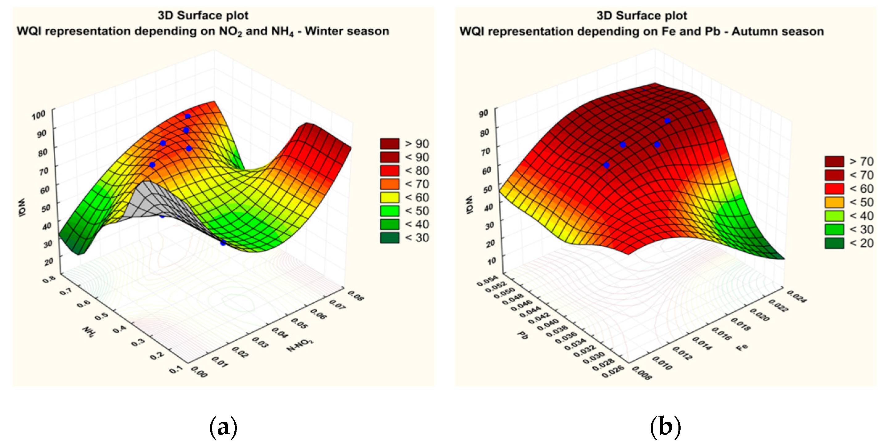
Further, based on this analysis, we were able to obtain surface model Plot type responses of the model response pattern for the parameter groups, which are closely correlated with the WQI in the data set studied. Thus, the estimated value for the WQI was represented on the vertical axis, and two parameters, which show correlations with the WQI size, were represented on the horizontal axis. Thus, for the winter season, there was a close connection between the WQI and NO₂⁻, respectively NH₄⁺, which were represented on the horizontal axis. Similarly, for the autumn season, a close relationship was noted between the values of the WQI and the concentration of Fe²⁺ and Pb²⁺, respectively. The PCA method is actually based on the use of values of correlation coefficients between data sets. Thus, considering the model response (RSM), a strong correlation was identified between the WQI and the NH₄⁺ and NO₂⁻ (Figure 5a) concentrations, on the one hand, and between the WQI and Fe-total and Pb²⁺ concentrations, on the other. These chemical parameters influence the values of the water quality index the most. In both cases studied—the WQI dependence of NH₄⁺ and NO₂⁻, respectively the WQI dependence on Fe-total and Pb²⁺, the surface obtained corresponds to dynamically equilibrium states with accumulation of representative points along a maximum curve/trajectory. This is explicable from a mathematical point of view, taking into account the values of the correlation coefficients closely between the selected magnitudes along the horizontal axes.

This suggests the existence of a dynamic equilibrium obtained by opposed processes which is, otherwise, encountered in the correlation matrix.

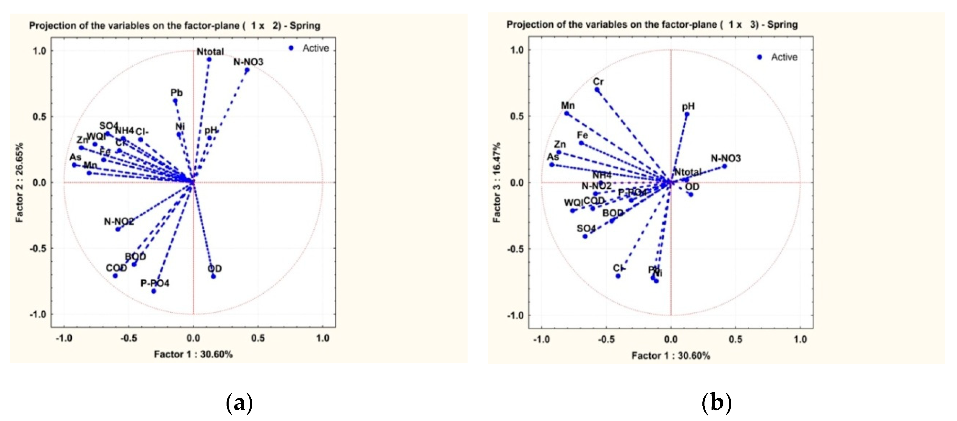
The PCA method (Figure 6) applied on the data recorded in the springs of the monitored years illustrates an obvious grouping into two different categories: group one formed of Fe²⁺, As²⁺, SO₄²⁻, Cr-total, SO₄²⁻, NH₄⁺ which correlates closely with the WQI (factor 1—horizontal axis) and group two including Pb²⁺, Ni²⁺, P-PO₄³⁻, N-total, NO₃⁻ (factor 2—vertical axis). The two factors explain 57% of the total variation.

Under the circumstances, a third factor had to be analyzed (Figure 6a). The related diagram shows that this third factor explains 16.47% of the total variation, and it groups the Pb²⁺, Cl⁻, Ni²⁺, pH, etc.

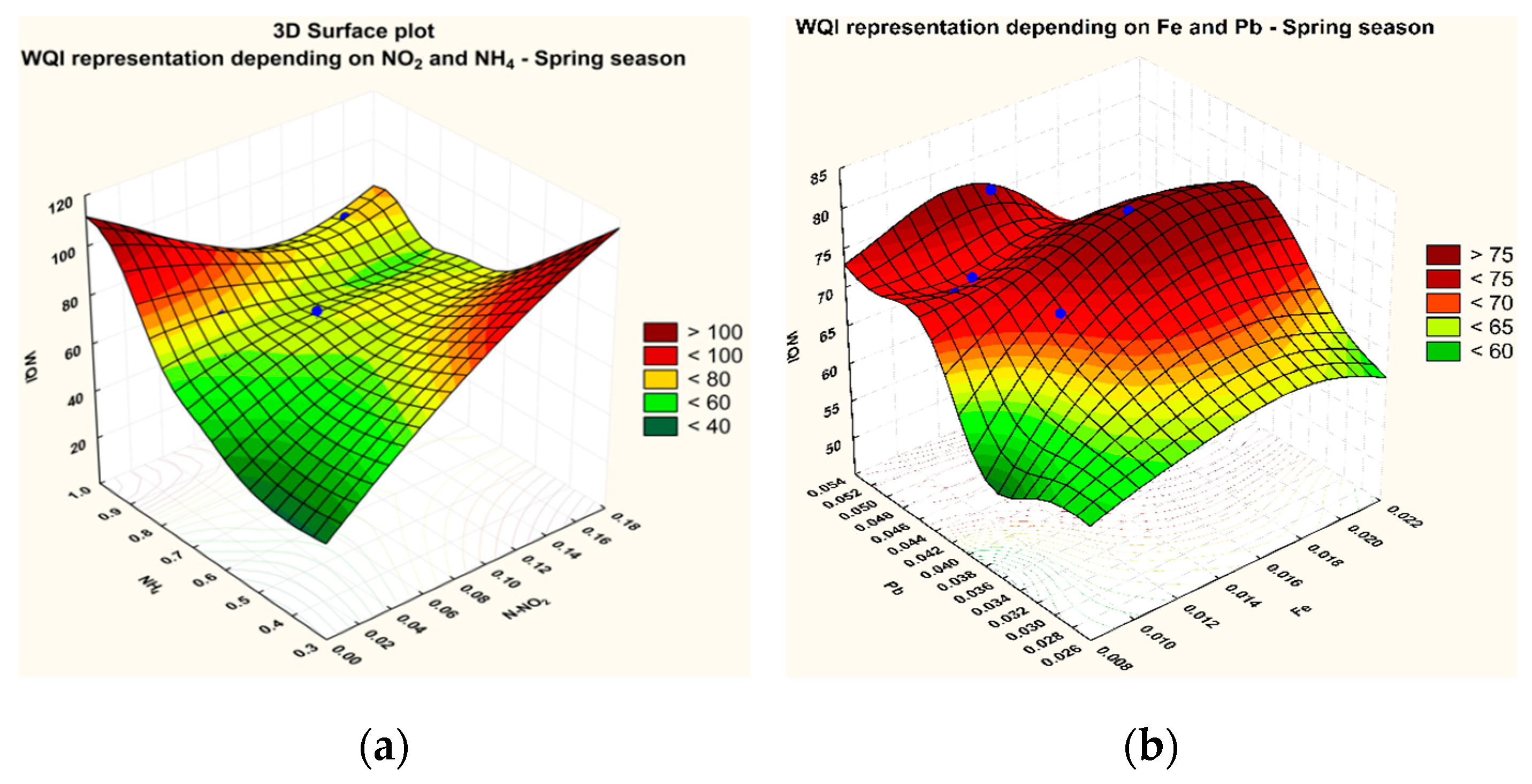
The RSM technique confirmed the existence of a correlation determined by the equilibrium between the WQI and NH₄⁺ and NO₂⁻, Fe-total and Pb²⁺ concentrations (Figure 7) as it resulted from the correlations of the matrix evaluation. As regards the dependence between the WQI and NH₄⁺ and NO₂⁻ concentrations (Figure 7a), a stable equilibrium surface shape could be noted. This aspect suggests a dynamic equilibrium which results from opposed processes [16]. The surface constructed by extrapolation may sometimes exceed 100 units for the WQI, but the representative points which are drawn in blue are certainly within the range of normal values for the WQI.

In the case of the WQI dependency and the Fe-total and Pb²⁺ concentrations (Figure 6b) the shape of the answer surface remains of the unstable equilibrium type, with representative points of accumulation along the maximum path curve. A maximum path curve in such situations was expected due to mathematical reasons [16]. This aspect suggests the existence of a dynamic equilibrium resulted from a series of opposed processes in which Fe-total and Pb²⁺ are involved. A numerical model for assessing chemical balance states and for analyzing the stability of these states is under construction and will be the subject of future research papers.

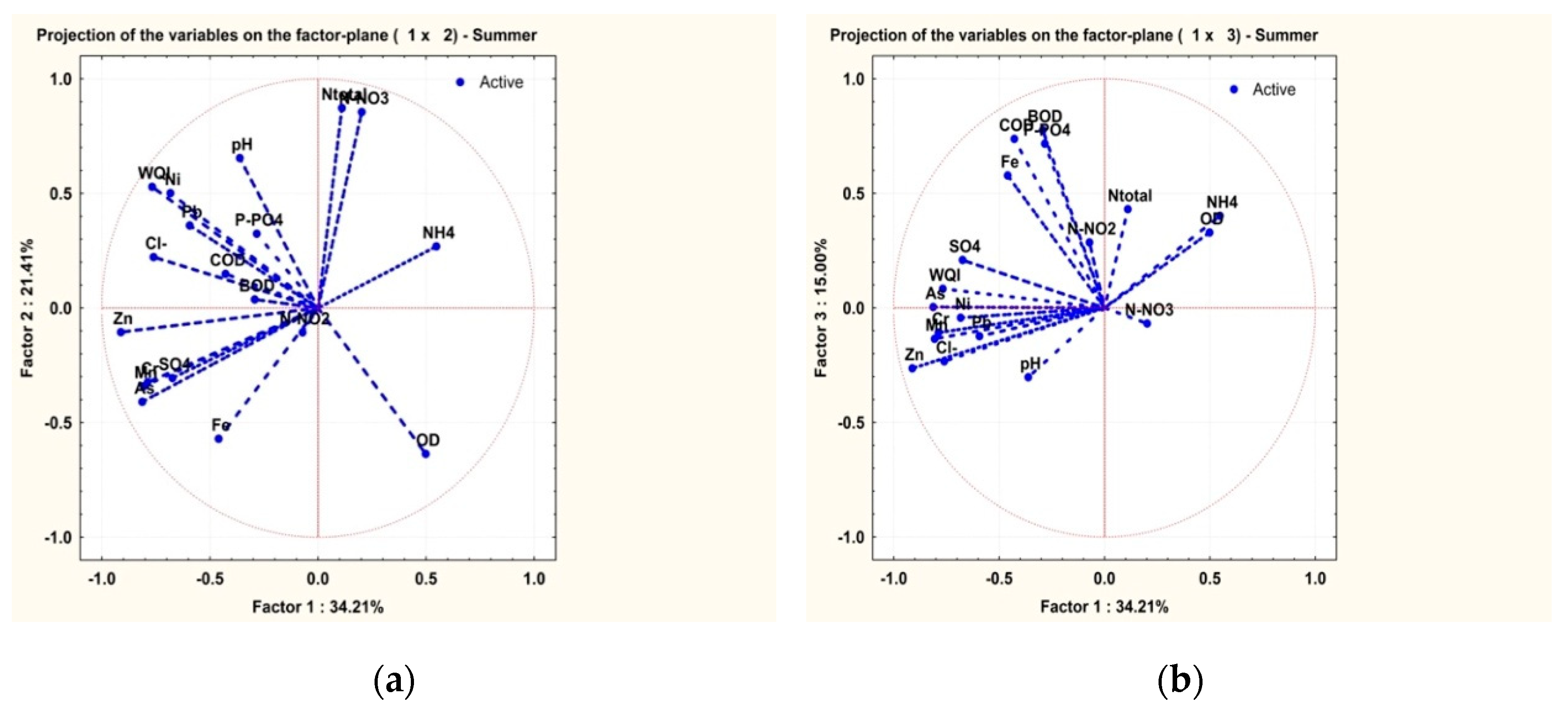
Different from the data recorded during the seasons of winter and spring, the data collected during the four summers of monitoring activities illustrate slightly different correlations. The PCA method emphasized the correlation between the WQI and the chemical parameters COD, BOD, Pb²⁺, Ni²⁺, Cl⁻, Zn²⁺, SO₄²⁻, which form the group factor 1 (F1) representing 34.21% of the option. Group factor 2 (F2) is made up of N-total, NO₃⁻, pH and represents 21.41%. Since these two factors represent only 56% of the option, a third component of the F3 factor had to be analyzed. The F3 factor represents 15% of the variation, the N-total, NO₂⁻ included in this group correlating negatively with the pH.

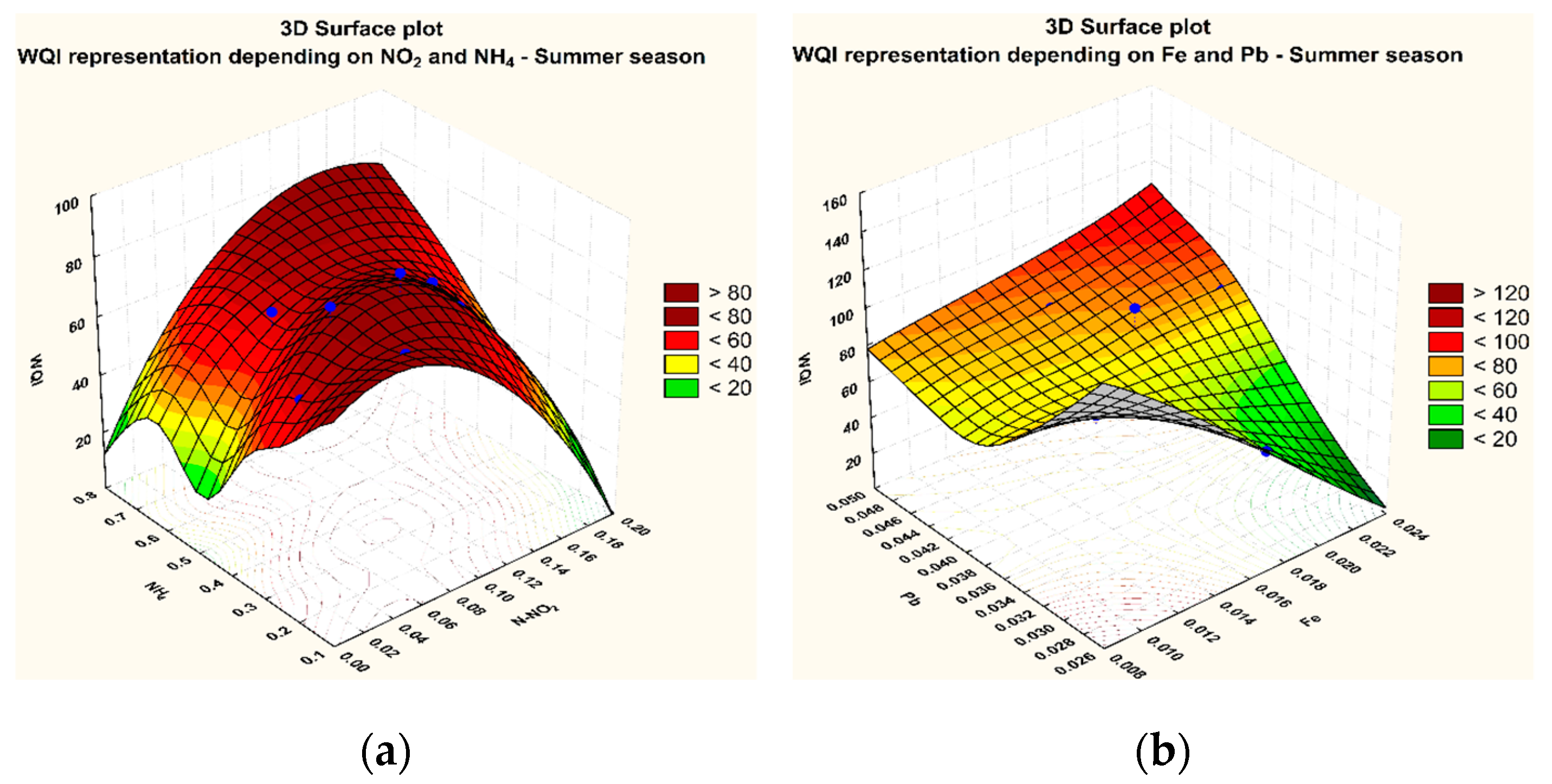
The variation of the WQI with the NH₄⁺ and NO₂⁻ concentrations and of the WQI with Fe-total and Pb²⁺ concentrations is also shown in the RSM diagram (Figure 7). In the case of the WQI and NH₄⁺ and NO₂⁻ concentrations (Figure 6a) there is an unstable equilibrium type of surface, this being a dynamic equilibrium between opposed processes, probably biological. As far as the dependence between the WQI and Fe-total and Pb²⁺ concentrations is concerned, (Figure 7b), there exists a stable equilibrium type of surface, this being a dynamic equilibrium between opposed processes which are correlated negatively.

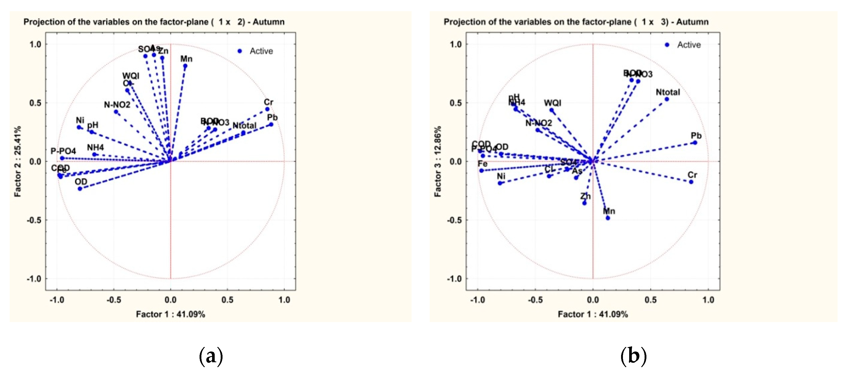
The analysis of the data collected during the four autumns illustrates a change in the interdependencies. This fact may be explained by the lower flow of the water stream recorded between the end of summer and the first two autumn months.

Figure 8a indicates the PCA analysis of the data collected in this season. The fact could be noticed that, at this time of the year, the WQI depends on Cl⁻, SO₄²⁻, As²⁺, Zn²⁺, Mn²⁺ and on NO₂⁻, the least. These parameters are now part of the factor group F2 which explains 25.41% of the variant. The factor group F1, which explains 41.09% of the variant, is made up of P-PO₄³⁻, NH⁴⁺, DO, COD, Fe²⁺, Ni²⁺ and is correlated negatively with BOD, N-total, Pb²⁺, Cr³⁺. These two factors explain over 65% of the total variance. The presence of factor 3 (F3) was also analyzed and it represents 12.86%, in this case. BOD si NO₃⁻ in factor group F3 are correlated negatively with Zn²⁺ and Mn²⁺.

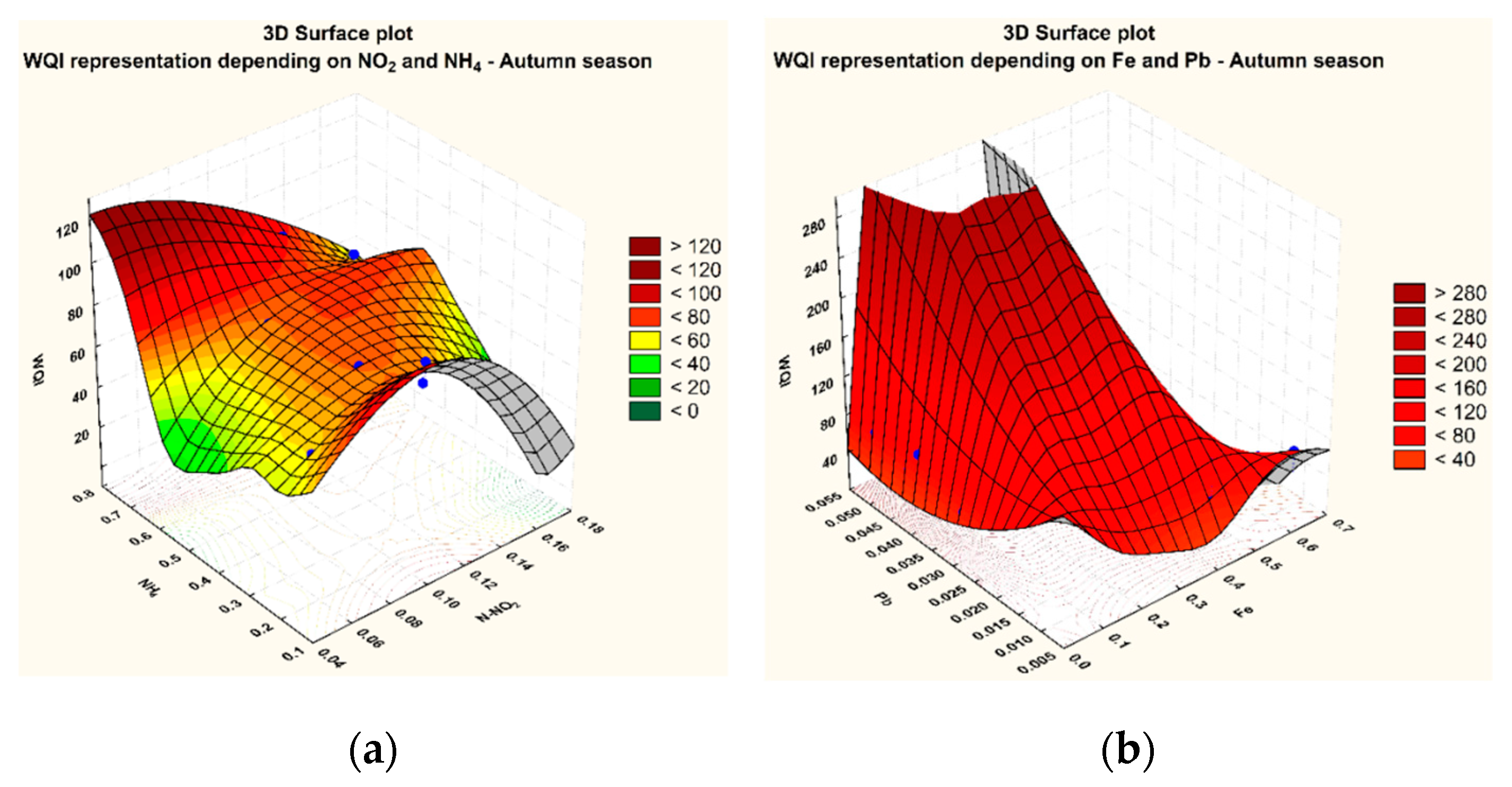
The analysis of the way in which the WQI varies depending on the NH⁴⁺ and NO₂⁻ concentrations and on Fe-total and Pb²⁺ concentrations is made by means of the RSM method (Figure 9).

The fact could be noticed that, as illustrated by the diagrams in Figure 10, the more concentrated the chemical species, the higher the WQI. These diagrams are characteristic to unstable dynamic equilibrium which favours reaching maximal values. The increase of the WQI over 100 may be explained by the fact that our research focused strictly on the dependence on the mentioned species, without taking into consideration the other 16 parameters. When the values of all the 18 physical and chemical parameters are introduced in the calculation of the WQI, the values decrease significantly under 100. However, the low water flow during autumn explains the higher values of the WQI as compared to the other seasons (Figure 10 and Figure 11).

4. Conclusions

The WQI values obtained describe accurately the state of the water stream. If the WQI is calculated in relation to 2–3 parameters, its value can increase or decrease significantly. Consequently, in order to assess the quality of a water stream correctly, more parameters was taken into account.

For large aquatic ecosystems as Danube river it is necessary to develop multiple experiments on large area and during long period (few years) in order to take into account, the maximum pollutants possible. In specials areas with large rivers and tributaries (as Danube is with Siret and Prut rivers) the experiments have to determinate also the influence of tributaries covering their own basins having specific anthropic impact.

The water samples were taken close to the right shore. Although there is an important intake of polluting substances from the affluent, the high water flow dilutes them significantly.

The water flow is important but it is not the only variable with a significant impact on water quality.

If we consider a steady anthropic impact consistent with constant pollutant loads, the concentration of the pollutants, reflected in the water quality, should depend exclusively on the flow. Diverse flow rates for the Danube generally include minimum values in the summer-autumn seasons. It may be noticed, however, that there are cases when the maximum WQI values, corresponding to an advanced pollution, are traceable during spring periods, when the flows are large enough to ensure a significant dilution for the pollutants. From the field observations, water intake during the spring season resulted from the melting of snow in the adjacent areas of the 3 rivers (the Siret, the Prut and the Danube). As it has been mentioned, these areas are characterized by important agricultural and industrial activities involving soil pollution, which explain the increase in pollutant concentrations even in the context of increased flow. These observations point to the need for integrated future studies which include both determinations of the pollution of adjacent soils and snow during the transition period between winter and spring for the correct identification of the origin of anthropogenic pollution.

The nutrients intake generally reaches the upstream of the monitored area, in our case the upstream of Rivers Siret and Prut. Studies made on these important rivers demonstrated that the concentration of some pollutants are higher as compared to the Danube ones [50,51]. Their conclusions correspond with the values observed in different stations (S2, S4) which have maximums superior compared to the other three stations.

The heavy metals intake was emphasized in areas sensitive to pollution: that is in the mineral harbour area and the ferry crossing area.

References

- Bojarczuk, A.; Jelonkiewicz, L.; Lenart-Boron, A. The effect of anthropogenic and natural factors on the prevalence of physicochemical parameters of water and bacterial water quality indicators along the river Białka, southern Poland. Environ. Sci. Pollut. Res. 2018, 25, 10102–10114. [Google Scholar] [CrossRef] [PubMed]
- Iticescu, C.; Georgescu, L.P.; Topa, C.M. Assessing the Danube Water Quality Index in the City of Galati, Romania, Carpath. J. Earth Environ. Sci. 2013, 8, 155–164. [Google Scholar] [CrossRef]
- Karabulut, A.; Egoh, B.N.; Lanzanova, D.; Grizzetti, B.; Bidoglio, G.; Pagliero, L.; Bouraoui, F.; Aloe, A.; Reynaud, A.; Maes, J.; et al. Mapping water provisioning services to supportthe ecosystem–water–food–energy nexus in the Danube river basin. Ecosyst. Serv. 2016, 17, 278–292. [Google Scholar] [CrossRef]
- Voza, D.; Vukovic, M.; Takic, L.; Nikolic, D.; Mladenovic-Ranisavljevic, I. Application of multivariate statistical techniques in the water quality assessment of Danube river, Serbia. Arch. Environ. Protect. 2015, 41, 96–103. [Google Scholar] [CrossRef] [Green Version]
- Stoica, C.; Lucaciu, I.; Nicolau, M.; Vosniakos, F. Monitoring the ecological diversity of the aquatic Danube Delta systems in terms of spatial- temporal relationship. J. Environ. Prot. Ecol. 2012, 13, 476–485. [Google Scholar]
- Caldararu, A.; Rosati, I.; Barbone, E.; Georgescu, L.P.; Iticescu, C.; Basset, A. Implementing European water framework directive: Uncertainty degree of metrics for macroinvertebrates in transitional waters. Environ. Eng. Manag. J. 2010, 9, 1259–1266. [Google Scholar] [CrossRef]
- Iticescu, C.; Murariu, G.; Georgescu, L.P.; Burada, A.; Ţopa, C.M. Seasonal variation of the physico-chemical parameters and Water Quality Index (WQI) of Danube water in the transborder Lower Danube area. Rev. Chim. (Buchar.) 2016, 67, 1843–1849. [Google Scholar]
- Dinka, M.O.; Loiskandl, W.; Ndambuki, J.M. Hydrochemical characterization of various surface water and ground water resources available in Matahara areas, Fantalle Woreda of Oromiya region. J. Hydrol. Reg. Stud. 2015, 3, 444–456. [Google Scholar] [CrossRef]
- El Hawary, A.; Shaban, M. Improving drainage water quality: Constructed wetlands-performance assessment using multivariate and cost analysis. Water Sci. 2018, 32, 301–317. [Google Scholar] [CrossRef] [Green Version]
- Iqbal, M.M.; Shoaib, M.; Agwanda, P.; Lee, J.L. Modeling approach for water-quality management to control pollution concentration: A case study of Ravi River, Punjab, Pakistan. Water 2018, 10, 1068. [Google Scholar] [CrossRef]
- Iqbal, M.M.; Shoaib, M.; Farid, H.U.; Lee, J.L. Assessment of water quality profile using numerical modeling approach in major climate classes of Asia. Int. J. Environ. Res. Public Health 2018, 15, 2258. [Google Scholar] [CrossRef] [PubMed]
- Rakotondrabe, F.; Ndam Ngoupayou, J.R.; Mfonka, Z.; Rasolomanana, E.H.; Nyangono Abolo, A.J.; Ako Ako, A. Water quality assessment in the Bétaré-Oya gold mining area (East-Cameroon): Multivariate Statistical Analysis approach. Sci. Total Environ. 2018, 610–611, 831–844. [Google Scholar] [CrossRef] [PubMed]
- Prasad, M.; Sunitha, V.; Sudharshan Reddy, Y.; Suvarna, B.; Muralidhara Reddy, B.; Ramakrishna Reddy, M. Data on water quality index development for groundwater quality assessment from Obulavaripalli Mandal, YSR district, A.P India. Data Brief 2019, 24, 103846. [Google Scholar] [CrossRef] [PubMed]
- Order 161/2006, The Normative on the Classification of Surface Water Quality in Order to Establish the Ecological s Romanian Ministry of Research and Innovation Tatus of Water Bodies; Official Monitor: Bucharest, Romania, 13 June 2006.
- Directive 2000/60/ec of the European Parliament and of the Council of 23 October 2000. Establishing a Framework for Community Water Policy. Available online: https://eur-lex.europa.eu/legal-content/RO/TXT/?uri=celex%3A32000L0060 (accessed on 16 June 2017).
- Popa, P.; Murariu, G.; Timofti, M.; Georgescu, L.P. Multivariate statistical analyses of water quality of Danube river at Galati, Romania. Environ. Eng. Manag. J. 2018, 17, 491–509. [Google Scholar]
- National Institute of Hydrology and Water Management Daily Reports. Available online: http://www.inhga.ro/diagnoza _si_prognoza_dunare (accessed on 20 May 2019).
- SR ISO 10523, 2009—Water Quality—Determination of pH; ISO: Geneva, Switzerland, 2009.
- SR EN 1899-2:2002—Water Quality—Determination of Biochemical Oxygen Demand after N Days (CBOn). Part 2: Method for Undiluted Samples; ISO: Geneva, Switzerland, 2002.
- SR EN ISO 6878:2005—Water Quality—Determination of Phosphorus. Spectrophotometric Method with Ammonium Molybdate; ISO: Geneva, Switzerland, 2005.
- SR EN ISO 11732:2005—Water Quality—Determination of Ammoniacal Nitrogen. Flow Analysis Method (CFA and FIA) and Spectrometric Detection; ISO: Geneva, Switzerland, 2005.
- ISO 15705:2002—Water Quality—Determination of the Chemical Oxygen Demand Index (ST-COD)—Small-Scale Sealed-Tube Method; ISO: Geneva, Switzerland, 2002.
- SR ISO 6777/1996—Water Quality—Determination of the Nitrogen from Nitrite Determination by Spectrometric Detection; ISO: Geneva, Switzerland, 1996.
- SR ISO 7890-3/2000—Water Quality—Determination of the Nitrogen from Nitrate Determination by Spectrometric Detection; ISO: Geneva, Switzerland, 2000.
- SR EN ISO 11905-1:2003—Water Quality—Determination of Nitrogen Content. Part 1: Oxidative Mineralization Method with Peroxodisulphate; ISO: Geneva, Switzerland, 2003.
- SR ISO 6332:1996/C91:2006—Water Quality—Determination of Iron Content. Spectrometric Method with 1,10—Phenanthroline; ISO: Geneva, Switzerland, 2006.
- SR ISO 9297/2001—Water Quality—Determination of Chloride Content. Titration with Silver Nitrate Using Chromate as Indicator (Mohr Method); ISO: Geneva, Switzerland, 2001.
- STAS 3069-87—Water Quality—Determination of Sulphate Content; ASRO: Bucharest, Romania, 2003.
- SR ISO 10566:2001—Surface Water and Wastewater—Determination of Lead; ISO: Geneva, Switzerland, 2001.
- SR ISO 9174-98—Water Quality—Determination of Cr Total—Spectrometric Method; ISO: Geneva, Switzerland, 1998.
- Clocotici, V. Introduction to Multivariate Statistics, Univ. Al. I. Cuza, Iasi, Faculty of Informatics. 2007. Available online: http://www.docstemplate.com/statistica-multivariata (accessed on 15 September 2016).
- Jianqin, M.; Jingjing, G.; Xiaojie, L. Water quality evaluation model based on principal component analysis and information entropy: Application in Jinshui River. J. Res. Ecol. 2010, 1, 249–252. [Google Scholar] [CrossRef]
- Garizi, A.Z.; Sheikh, V.; Sadoddin, A. Assessment of seasonal variations of chemical characteristics in surface water using multivariate statistical methods. Int. J. Environ. Sci. Technol. 2011, 8, 581–592. [Google Scholar] [CrossRef] [Green Version]
- Kebede, Y.K.; Kebede, T. Application of Principal Component Analysis in Surface Water Quality Monitoring. In Principal Component Analysis—Engineering Applications; Sanguansat, P., Ed.; IntechOpen: London, UK, 2012; pp. 83–100. [Google Scholar]
- Giordano, G. A new dimension in the factorial techniques: The response surface. Stat. Appl. 2006, 18, 359–373. [Google Scholar]
- Jiménez-Contreras, E.; Torres-Salinas, D.; Bailón Moreno, R.; Ruiz Baños, R.; Delgado López-Cózar, E. Response Surface Methodology and its application in evaluating scientific activity. Scientometrics 2008, 79, 201–218. [Google Scholar] [CrossRef] [Green Version]
- Kaurish, F.W.; Younos, T. Developing a standardized water quality index for evaluating surface water quality. J. Am. Water Resour. Assoc. 2007, 3, 533–545. [Google Scholar] [CrossRef]
- Takic, L.M.; Mladenovic-Ranisavljevic, I.I.; Nikolic, V.D.; Nikolic, L.B.; Vukovic, M.V.; Zivkovic, N.V. The assessment of the Danube water quality in Serbia. Adv. Technol. 2012, 1, 58–66. [Google Scholar]
- Water Pollution Control—A Guide to the Use of Water Quality Management Principles; Helmer, R.; Hespanhol, I. (Eds.) F & FN Spon: London, UK, 1997. [Google Scholar]
- Ayeni, O.; Soneye, A.S.O. Interpretation of surface water quality using principal components analysis and cluster analysis. J. Geogr. Reg. Plan. 2013, 6, 132–141. [Google Scholar] [CrossRef]
- Burada, A.; Topa, C.M.; Georgescu, L.P.; Teodorof, L.; Nastase, C.; Seceleanu-Odor, D.; Iticescu, C. Heavy Metals Environment Accumulation in Somova—Parches Aquatic Complex from the Danube Delta Area. Rev. Chim. (Buchar.) 2015, 66, 48–54. [Google Scholar]
- Ţopa, M.C.; Timofti, M.; Burada, A.; Iticescu, C.; Georgescu, L.P. Danube water quality during and after flood near an urban agglomeration. J. Environ. Prot. Ecol. 2015, 16, 1255–1261. [Google Scholar]
- Pintilie, V.; Ene, A.; Georgescu, L.P.; Moraru, L.P.; Iticescu, C. Measurements of gross alpha and beta activity in drinking water from Galati region, Romania. Rom. Rep. Phys. 2016, 68, 1208–1220. [Google Scholar]
- Rodríguez-Romero, A.J.; Rico-Sánchez, A.E.; Mendoza-Martínez, E.; Gómez-Ruiz, A.; Sedeño-Díaz, J.E.; López-López, E. Impact of Changes of Land Use on Water Quality, from Tropical Forest to Anthropogenic Occupation: A Multivariate Approach. Water 2018, 10, 1518. [Google Scholar] [CrossRef]
- Tyagi, S.; Sharma, B.; Singh, P.; Dobhal, R. Water Quality Assessment in Terms of Water Quality Index. Am. J. Water Resour. 2013, 1, 34–38. [Google Scholar]
- Iticescu, C.; Georgescu, L.P.; Topa, C.; Murariu, G. Monitoring the Danube Water Quality near the Galati City. J. Environ. Prot. Ecol. 2015, 15, 30–38. [Google Scholar]
- Timofti, M.; Popa, P.; Murariu, G.; Georgescu, L.; Iticescu, C.; Barbu, M. Complementary approach for numerical modelling of physicochemical parameters of the Prut River aquatic system. J. Environ. Prot. Ecol. (JEPE) 2016, 1, 53–63. [Google Scholar]
- Chowdhury, R.M.; Muntasir, S.Y.; Hossain, M.M. Water quality index of water bodies along Faridpur-Barisal road in Bangladesh. Glob. Eng. Technol. Rev. 2012, 2, 1–8. [Google Scholar]
- Mena-Rivera, L.; Salgado-Silva, V.; Benavides-Benavides, C.; Coto-Campos, J.M.; Swinscoe, T.H.A. Spatial and Seasonal Surface Water Quality Assessment in a Tropical Urban Catchment: Burío River, Costa Rica. Water 2017, 9, 558. [Google Scholar] [CrossRef]
- Georgescu, P.L.; Voiculescu, M.; Dragan, S.; Timofti, M.; Caldararu, A. Study of spatial and temporal variations of some physic-chemical parameters of Lower Siret River. J. Environ. Prot. Ecol. 2010, 11, 837–844. [Google Scholar]
- Voiculescu, M.; Georgescu, P.L.; Dragan, S.; Timofti, M.; Caldararu, A. Study of anthropogenic effects on the quality of Lower Prut River. J. Environ. Prot. Ecol. 2011, 12, 16–24. [Google Scholar]
Figure 1.
Distribution of sampling points.
Figure 3.
The seasonal variation of the WQI in the 5 sampling points during the winter of 2013–the winter of 2016 (Series 1 corresponding with Sampling point 1; Series 2 corresponding with Sampling point 2 etc.).
Figure 4.
PCA for WQI and physicochemical parameters in the winter seasons of 2013 to 2016. (a) correlation F2–F1; (b) correlation F3–F1.
Figure 5.
RSM for the WQI = f(NH4+, NO2−) (a) and the WQI = f(Fe-total, Pb2+); (b) for the winter seasons of 2013 to 2016.
Figure 6.
PCA of the WQI and of the physicochemical parameters in the spring seasons of 2013 to 2016. (a) correlation F2–F1; (b) correlation F3–F1.
Figure 7.
RSM for the WQI = f(NH4+, NO2−) (a) and the WQI = f(Fe-total, Pb2+); (b) in the summer seasons of 2013 to 2016.
Figure 8.
PCA for the WQI and the physicochemical parameters in the summer seasons of 2013 to 2016. (a) correlation F2–F1; (b) correlation F3–F1.
Figure 9.
Figure 10.
PCA for the WQI and the physicochemical parameters in the autumn seasons of 2013 to 2016. (a) correlation F2–F1; (b) correlation F3–F1.
Figure 11.
RSM for the WQI = f(NH4+, NO2−) (a) and the WQI = f(Fe-total, Pb2+); (b) in the autumn seasons of 2013 to 2016.