Interplays between State and Flux Hydrological Variables across Vadose Zones: A Numerical Investigation

1
Institute of Surface-Earth System Science, Tianjin University, Weijin Road 92, Tianjin 300072, China
2
Tianjin Key Laboratory of Earth Critical Zone Science and Sustainable Development in Bohai Rim, Tianjin University, Weijin Road 92, Tianjin 300072, China
*
Author to whom correspondence should be addressed.
Water 2019, 11(6), 1295; https://doi.org/10.3390/w11061295
Submission received: 17 May 2019
/
Revised: 15 June 2019
/
Accepted: 16 June 2019
/
Published: 20 June 2019
(This article belongs to the Special Issue Water Flow, Solute and Heat Transfer in Groundwater)
Abstract
:Knowledge of both state (e.g., soil moisture) and flux (e.g., actual evapotranspiration (ETa) and groundwater recharge (GR)) hydrological variables across vadose zones is critical for understanding ecohydrological and land-surface processes. In this study, a one-dimensional process-based vadose zone model with generated soil hydraulic parameters was utilized to simulate soil moisture, ETa, and GR. Daily hydrometeorological data were obtained from different climate zones to drive the vadose zone model. On the basis of the field phenomenon of soil moisture temporal stability, reasonable soil moisture spatiotemporal structures were reproduced from the model. The modeling results further showed that the dependence of ETa and GR on soil hydraulic properties varied considerably with climatic conditions. In particular, the controls of soil hydraulic properties on ETa and GR greatly weakened at the site with an arid climate. In contrast, the distribution of mean relative difference (MRD) of soil moisture was still significantly correlated with soil hydraulic properties (most notably residual soil moisture content) under arid climatic conditions. As such, the correlations of MRD with ETa and GR differed across different climate regimes. In addition, the simulation results revealed that samples with average moisture conditions did not necessarily produce average values of ETa and GR (and vice versa), especially under wet climatic conditions. The loose connection between average state and flux hydrological variables across vadose zones is partly because of the high non-linearity of subsurface processes, which leads to the complex interactions of soil moisture, ETa, and GR with soil hydraulic properties. This study underscores the importance of using soil moisture information from multiple sites for inferring areal average values of ETa and GR, even with the knowledge of representative sites that can be used to monitor areal average moisture conditions.
1. Introduction
Estimation of state (e.g., soil moisture) and flux (e.g., actual evapotranspiration (ETa) and groundwater recharge (GR)) hydrological variables across vadose zones are of great importance for many research and application purposes, and especially for understanding ecohydrological and land-surface processes in Earth’s critical zones [1,2,3]. Due to the high non-linearity and extreme complexity of hydrological systems, those state and flux variables tend to display significant spatiotemporal variability. For example, a wealth of field and numerical studies has shown that there was considerable variability in soil moisture at different spatiotemporal scales, as a result of its complex interactions with surrounding environments [4,5]. Likewise, flux hydrological variables, such as ETa and GR, may also vary substantially across landscapes, largely because of the marked spatial variations in soil texture, vegetation, and climatic conditions [1,6,7,8,9]. As such, accurate estimation of those state and flux variables presents grand challenges to scientific communities [10,11,12,13]. Given the tight connections between state and flux variables [12,14,15], it is thus imperative to elucidate the interplays among those variables to improve their estimation across vadose zones.
To enhance the representativeness of estimation of state and flux hydrological variables across vadose zones, various techniques have been developed [6,16,17]. Notably, in the field of soil hydrology, the method of temporal stability analysis (TSA) initially proposed by Vachaud et al. [18] has been widely adopted to identify representative locations for monitoring soil moisture conditions [19]. Based on field observations, Vachaud et al. [18] found that there was a temporal persistence in the spatial structure of soil moisture. Specifically, Vachaud et al. [18] showed that soil moisture levels at certain locations in a field were closer to the areal average moisture conditions, whereas other locations consistently displayed either drier or wetter conditions than the areal average moisture conditions. As such, Vachaud et al. [18] suggested that it was feasible to apply the TSA method, which is based on the metric of mean relative difference (MRD) of soil moisture (an indicator of the relative wetness at a location as compared to the areal average wetness), to seek representative sites for monitoring areal average moisture conditions (e.g., sites with MRD values closest to zero). Since the seminal work of Vachaud et al. [18], the use of the TSA method has also been extended to optimize soil moisture monitoring networks, diagnose soil moisture spatiotemporal patterns, fill missing soil moisture data, and improve the practice of water resources management [20,21,22,23,24].
Despite its wide applications, the implication of the TSA method for understanding flux hydrological variables across vadose zones has not been adequately addressed. In general, the availability of field measurements of ETa and GR is extremely limited due to the high operational and maintenance costs of measurement equipment [3,25]. As an effective alternative to resolve this issue, soil moisture data have been used to infer ETa and GR, such as through inverse modeling [15,26,27]. Given the significant spatial variability in ETa and GR, it naturally leads to the question as to whether soil moisture data from representative locations identified by the TSA method can be used to infer areal average values of ETa and GR. To answer this question, it requires the knowledge of the relationships of soil moisture with ETa and GR. Although previous modeling studies have revealed that soil moisture, ETa, and GR were affected by similar factors (e.g., soil, vegetation, and climate), the dependence of those variables on environmental factors might vary considerably [9,28,29]. Therefore, further investigation into the interplays among soil moisture, ETa, and GR is still warranted.
The primary goals of this study were two-fold: (1) to investigate the relationships of soil moisture with ETa and GR under different climatic conditions and (2) to examine whether soil samples with average moisture conditions can also produce average hydrological fluxes, such as ETa and GR, across vadose zones. To this end, a commonly used process-based vadose zone model with generated soil hydraulic parameters was utilized to simulate soil moisture, ETa, and GR, as this type of modeling approach has been widely adopted for understanding hydrological processes across vadose zones (e.g., Vereecken et al. [30]; Wang et al. [31]; Martinez et al. [28]; also see the review by Vereecken et al. [5]). Based on the simulation results, the distribution patterns of MRD, ETa, and GR were first discussed, and then the correlations of MRD with ETa and GR were examined to understand the interdependence of those variables on climatic conditions and soil hydraulic properties. Finally, with the aid of the TSA method, the feasibility of using representative locations of soil moisture for estimating areal average values of ETa and GR was evaluated.
2. Methods and Materials
2.1. Model Setup and Data Inputs
The widely used Hydrus-1D model [32] was employed in this study to simulate soil moisture, ETa, and GR, due to the accuracy of its numerical algorithm [33]. The Hydrus-1D model is a one-dimensional process-based vadose zone model, which utilizes the Richards equation to simulate soil water movement in vadose zones:
where θ (L3/L3) is volumetric soil moisture content, t (T) is time, x (L) is spatial coordinate, h (L) is pressure head, K (L/T) is hydraulic conductivity, and S (1/T) is a sink/source term (e.g., root water uptake). To be concise, only brief information on the model setup is given here, and detailed mathematical descriptions of the simulated processes can be found in Simunek et al. [32]. Specifically, the length of the simulated soil columns was set to be 3 m with a total of 301 spatial nodes evenly distributed at 1 cm intervals. Additional numerical experiments showed that further increases in the number of the spatial nodes did not improve the simulation results. At the surface, an atmospheric boundary condition was chosen for calculating actual soil evaporation (Ea), which primarily depended on potential soil evaporation (Ep) and a predefined pressure head at the surface [34]. Surface runoff was allowed to occur when precipitation (P) intensity was greater than the soil infiltration capacity or the surface soil layer became saturated. A unit hydraulic gradient condition was imposed at the lower boundary of the simulated soil columns. As such, GR is defined here as the amount of water that passes downward across the lower boundary [6,31].
The method of Feddes et al. [35] was used to compute root water uptake, which depended on potential transpiration (Tp), soil matric potential, and root density distribution. Note that root water uptake was assumed to be equal to actual transpiration (Ta) in this study. Daily potential transpiration Tp was obtained by partitioning daily potential evapotranspiration (ETp) into Tp and Ep according to Beer’s law [36]:
where k is an extinction coefficient (0.5 in this study) and LAI is leaf area index. Following Wang and Zlotnik [37], LAI data were retrieved from the MODIS_MOD15 dataset [38] based on the geographical coordinates of the study sites. The exponential model of Jackson et al. [39] was adopted to describe the root density distribution according to the vegetation types at the study sites. Finally, the sum of Ea and Ta was set to be equal to ETa.
Ep = ETp × e-k×LAI
Tp = ETp − Ep
Instead of generating synthetic data to drive the Hydrus-1D model [28,40], five years of daily hydrometeorological data from four study sites with contrasting hydroclimatic conditions across China were obtained from the National Centers for Environmental Information [41], including Hangzhou, Guiyang, Tianjin, and Yinchuan. Specifically, the climates at Hangzhou and Guiyang are humid and sub-humid, respectively. By comparison, Tianjin is located in a semi-arid climate zone, while Yinchuan is located in an arid climate zone. First, daily P and maximum and minimum air temperatures were retrieved for each site. Given the data availability, the Hargreaves equation was used to calculate daily ETp based on maximum and minimum air temperatures [42]. The summary of mean annual P () and mean annual ETp () during the study period is provided in Table 1 for the four sites. Based on the land cover of the study sites, forest was assumed at Hangzhou and Guiyang, while grass and shrub were assumed at Tianjin and Yinchuan, respectively. Physiological parameter values for different vegetation types, which were used for computing root water uptake, were obtained from literature [43,44,45]. Finally, to minimize the impact of initial conditions on the simulation results, all simulations were repeated for four times (i.e., a total of 20 years) until the simulated soil moisture profiles were in equilibrium with atmospheric forcings, and the simulation results from the last repetition were used in the analysis.
2.2. Generation of Soil Hydraulic Parameters
To solve Equation (1), the constitutive relations among θ, h, and K are required. In this study, the van Genuchten–Mualem (VGM) model [46,47] was utilized:
where θr (L3/L3) and θs (L3/L3) are residual and saturated soil moisture content, respectively, KS (L/T) is saturated hydraulic conductivity, and Se (-) is effective saturation degree that is defined as (θ − θr)/(θs − θr). The parameters α, n, and l are shape factors: α(1/L) is related to the inverse of air entry pressure, n (-) is a measure of pore size distributions with m = 1 − 1/n, and l (-) is a measure of pore tortuosity and connectivity.
K(h) = KS × Sel × (1 − (1 −Se1/m) m)2
In previous modeling studies, because of the lack of field data, synthetic soil hydraulic parameter datasets have been routinely used to characterize the spatial variability in soil hydraulic properties for simulating soil moisture, ETa, and GR [9,28,48,49]. Here, the method of Zhang and Schaap [50] was utilized to generate the VGM parameters for loamy sand, sandy loam, and silt loam. This method is built on the assumption of either normal (θr and θs) or lognormal (α, n, and Ks) distributions of the VGM parameters. The validity of this assumption has been verified by Zhang and Schaap [50]. Based on a Monte Carlo procedure, new samples were drawn from the parameter (normal or lognormal) distributions with means and standard deviations given by Zhang and Schaap [50] for each soil texture class. In addition, following Wang et al. [31] and Zhang et al. [51], the parameter l was fixed to be 0.5 in all simulations. In this study, a total of 200 samples were generated for each soil texture class and the statistical summary of the generated VGM parameters is provided in Table 2. Note that soil profiles with uniform soil textures were used in this study. The main purpose of using uniform soil profiles is to promote general understanding, and thus reach general conclusions regarding the impact of soil hydraulic properties on subsurface hydrological processes. By comparison, the use of non-uniform soil profiles might lead to site-specific conclusions (as done in the majority of field-scale soil moisture studies), which, however, deserves future investigation based on numerical approaches.
2.3. Temporal Stability Analysis of Soil Moisture
Given its wide applications for analyzing soil moisture spatiotemporal patterns [19,52,53], the TSA method was adopted in this study to examine the relationships of soil moisture with ETa and GR. The TSA method is based on the metric of relative difference (RD) of soil moisture, which is defined as:
where θij is soil moisture content at location i and time j, and is the spatial average of soil moisture content at time j. With a series of RD over time, MRD at location i is given as:
where m is the number of observations over the study period. By definition, the term MRD characterizes the wetness condition at a location relative to the areal average wetness condition of the study field over the study period. Therefore, MRD can be used to characterize the spatial distribution of soil moisture (average state) and the sites with MRD values closest to zero can be selected as representative locations for monitoring field average moisture conditions [18,19].
The standard deviation of RD (SDRD) is another useful metric for quantifying soil moisture temporal dynamics and defined as:
According to its definition, sites with lower SDRD values indicate higher temporal stability of soil moisture than those with higher SDRD values. Note that instead of using soil moisture storage in this study, daily volumetric soil moisture content at 25 cm extracted from the last repetition of the simulations was analyzed. Since soil moisture storage is equivalent to depth-weighted soil moisture content and similar simulation results were obtained from other depths (e.g., 10, 50, and 100 cm), the conclusions made in this study essentially remain the same based on depth-specific simulation data. In addition, the use of depth-specific data is to be consistent with the framework set for soil moisture monitoring networks (e.g., Nebraska Mesonet, Oklahoma Mesonet, and Soil Climate Analysis Network), which report soil moisture data at different soil depths.
3. Results and Discussion
3.1. Comparison of Hydroclimatic Conditions across the Study Sites
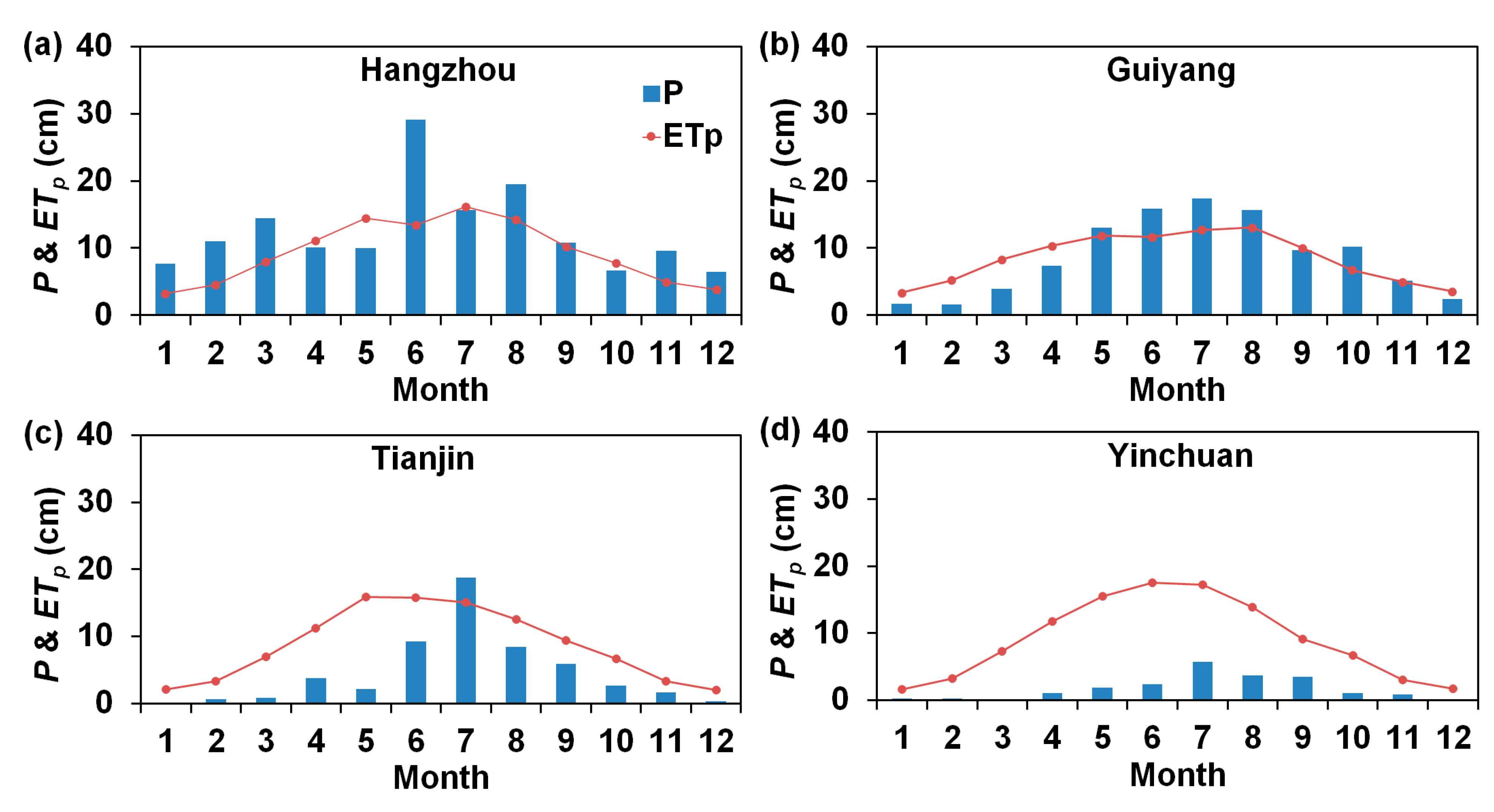
The statistical summary of and during the study period is reported in Table 1 for the study sites. Among the four sites, there was a significant gradient in increasing from 20.8 cm/year at Yinchuan to 150.9 cm/year at Hangzhou; whereas, the spatial variations in were much smaller with a range from 101.7 cm/year at Guiyang to 111.8 cm/year at Hangzhou. As a result, a wide range of mean annual aridity index (i.e., ) existed across the sites, varying from 0.74 at Hangzhou to 5.22 at Yinchuan. Given the diversity of climate regimes among the selected sites (e.g., from arid to humid climates), mean annual ratios of ETa (defined as ) and GR () were used in the following analysis to ensure the comparability of the simulated patterns of ETa and GR at different sites. With regard to the interannual variability, there were also pronounced variations in annual P at all sites; however, the interannual variability in ETp was less significant (Table 1). It should be noted that climate seasonality is another important climatic factor that affects ETa and GR [40,54]. Therefore, to examine the climate seasonality at the study sites, mean monthly P and ETp during the five-year study period are plotted in Figure 1. It can be seen from Figure 1 that the climates at the sites exhibited similar seasonal patterns with highest P and ETp occurring during summer months. As such, it is reasonable to argue that climate seasonality did not exert a significant impact on the comparison of the distribution patterns of the simulated and across the sites in this study.
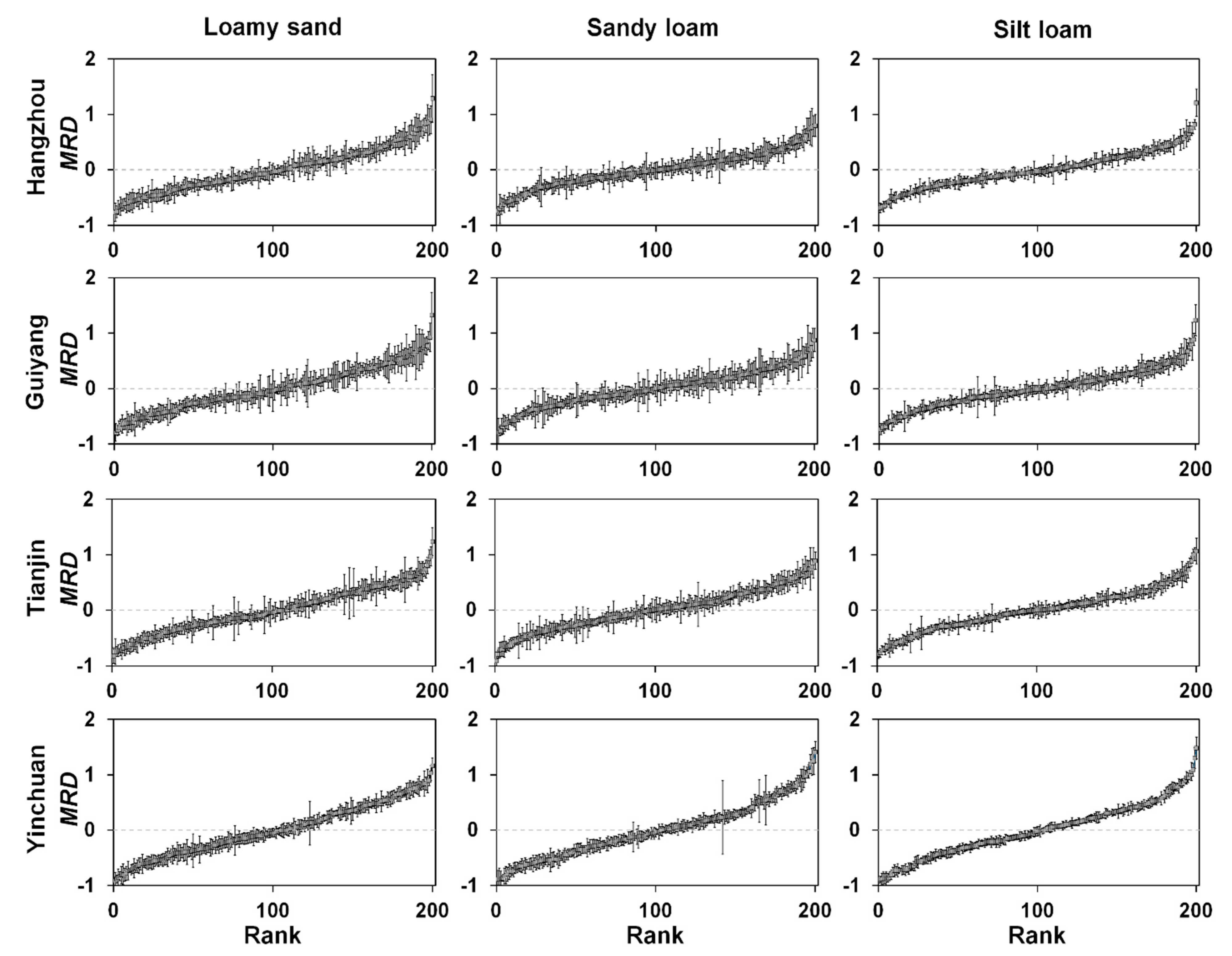
3.2. Simulated Patterns of MRD
To investigate the relationships of soil moisture with ETa and GR on the basis of the TSA method, it is necessary to first examine whether simulated soil moisture data could mimic the field phenomenon of soil moisture temporal stability as shown in previous field studies. To this end, Figure 2 shows the ranked MRD with associated SDRD obtained for different soil textures at the study sites. As previously explained, only soil moisture data simulated at 25 cm were used to compute MRD and SDRD in Figure 2. In general, the simulated MRD patterns were similar to those derived from field observations at various spatiotemporal scales [20,21,22,23,24]. In particular, Figure 2 shows that certain samples displayed consistently wetter soil moisture conditions (i.e., with larger MRD values) than others. More importantly, the ranges of both MRD and SDRD were in line with previously reported values obtained at watershed and regional scales [24,53,55]. For example, the range of MRD for loamy sand was from −0.765 to 1.287 at Hangzhou, from −0.797 to 1.324 at Guiyang, from −0.819 to 1.237 at Tianjin, and from −0.912 to 1.166 at Yinchuan (Table 3). It should be emphasized that there were variations in the statistical characteristics of MRD and SDRD produced by different modeling studies [28,29], which could be largely attributed to the differences in the synthetic soil hydraulic parameter datasets and hydrometeorological conditions used for simulations.
It is worth noting that inconsistent findings have been reported from previous studies regarding the environmental conditions and factors that mainly control soil moisture temporal stability. For example, there still exists a debate on whether soil moisture is temporally more stable under wetter or drier conditions [29,52,56]. In this study, the average soil moisture temporal stability as indicated by mean SDRD values varied noticeably among the sites (Table 3). It appears that soil moisture tended to be temporally more stable under both very wet (e.g., Hangzhou) and dry (e.g., Yinchuan) climatic conditions, while soil moisture temporal stability was lowest under intermediate climatic conditions (e.g., Guiyang). This result is in general agreement with the conclusion made by Lawrence and Hornberger [48], who showed that the observed soil moisture variability peaked in temperature regions with intermediate moisture conditions. Soil moisture levels remain high in humid regions due to the constant P inputs, which results in less temporal dynamics of soil moisture. In contrast, because of infrequent rainfall events in arid regions, soil moisture is also temporally less dynamic. Thus, it leads to the lowest soil moisture temporal stability at the sites with intermediate climatic conditions (e.g., in sub-humid regions).
Table 3 also reveals that mean SDRD values differed for different soil textures under the same climatic condition. For example, mean SDRD values were comparably smaller for silt loam than those for loamy sand and sandy loam at all sites. Based on a theoretical framework, Vereecken et al. [30] showed that the variability in soil hydraulic parameters could significantly affect soil moisture variability. From Table 2, it can be seen that the lower mean SDRD values for silt loam were mostly due to the smaller variability in the parameters α and KS. It, thus, corroborates our previous conjecture that the statistical characteristics of MRD and SDRD produced by synthetic modeling approaches are partly dependent on the variability in soil hydraulic parameters generated for simulations. In summary, the results from the TSA demonstrate the viability of using synthetic modeling approaches for reproducing reasonable spatiotemporal structures of soil moisture as observed in the fields.
3.3. Distribution Patterns of and
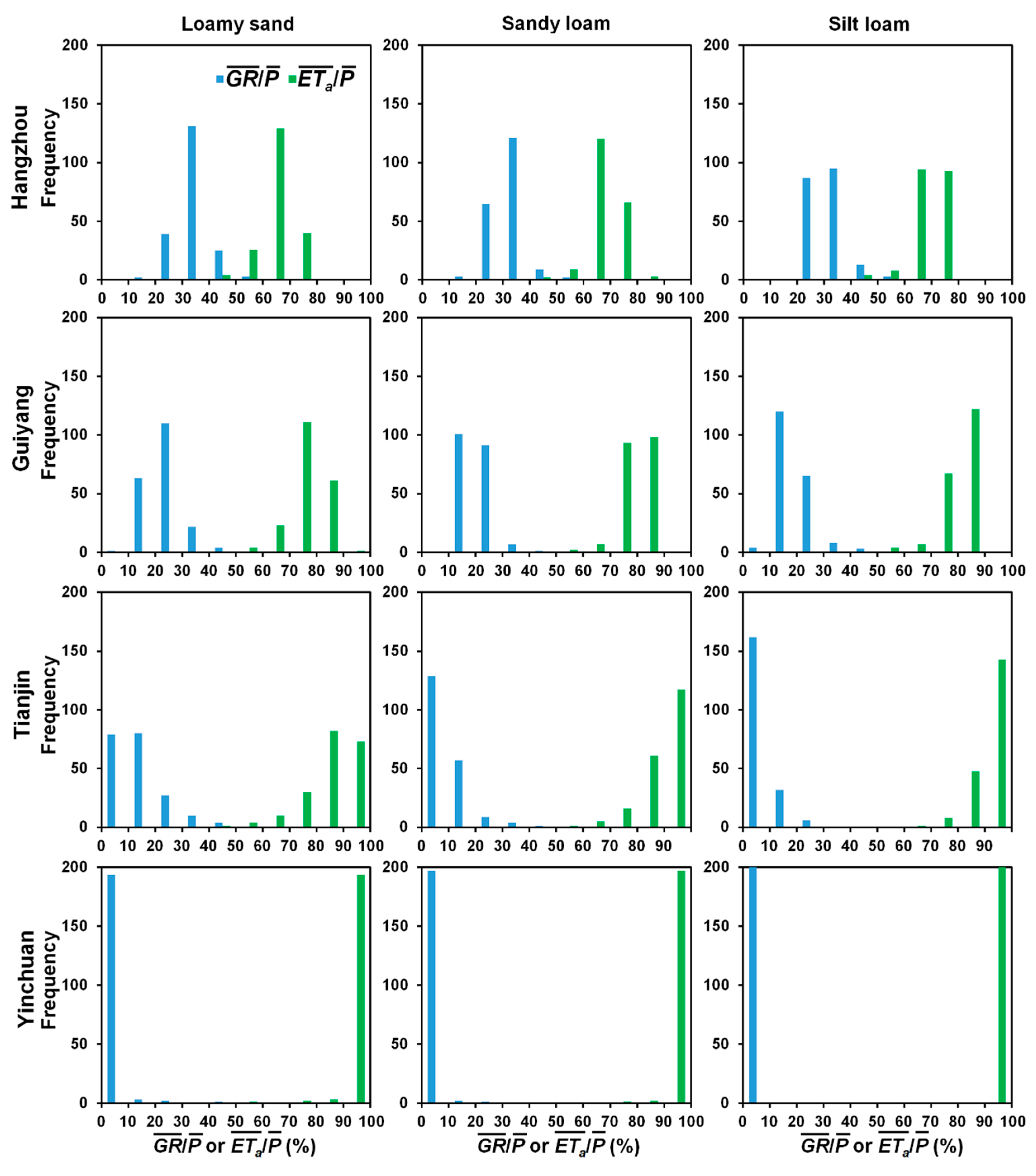
Following Wang et al. [31], histograms of simulated and , as shown in Figure 3, are used to discern the differences in the distribution patterns of and under different climatic conditions and for different soil textures. For the same soil texture, Figure 3 reveals that the ranges of and varied noticeably among the study sites. In particular, the distribution of increased towards the higher end of the range between 0 and 100% with increasing climate dryness, and the distribution of exhibited an opposite trend. This modeling result suggests that becomes progressively larger while grows gradually less important from humid to arid sites, which is consistent with the general understanding of the climate effect on ETa and GR [57]. Rainfall water infiltrated into soils needs to first satisfy the atmospheric demand for ETa before becoming GR. Thus, the opportunity for the infiltrated water to be evapotranspired is much higher under drier climatic conditions due to the higher atmospheric demands for evapotranspiration, resulting in the increasing trend in with increasing climate dryness.
Although the respective ranges were similar for and under the same climatic conditions, there were noticeable variations in the distribution patterns of and for different soil textures (Figure 3). In the order of loamy sand, sandy loam, and silt loam, there were proportionally more samples with higher (or lower ) values towards the higher (or lower) end of the distribution ranges, most notably at the sites of Hangzhou, Guiyang, and Tianjin. It reflects the controls of soil hydraulic properties on ETa and GR processes. Due to the higher infiltration capacities (e.g., Table 2 shows that Ks becomes gradually smaller from loamy sand to sandy loam and silt loam), coarser soils tend to produce lower and higher ratios [40,58]. Interestingly, at the site of Yinchuan with very dry climatic conditions, the contrast in the distribution patterns of and was less obvious among different soil textures. Regardless of soil textural differences, most of P becomes ETa in arid regions due to the limited water supplies, which greatly weakens the dependence of ETa and GR on soil hydraulic properties. It, thus, suggests that the controls of soil hydraulic properties on ETa and GR vary with climatic conditions.
3.4. Relationships of MRD with and
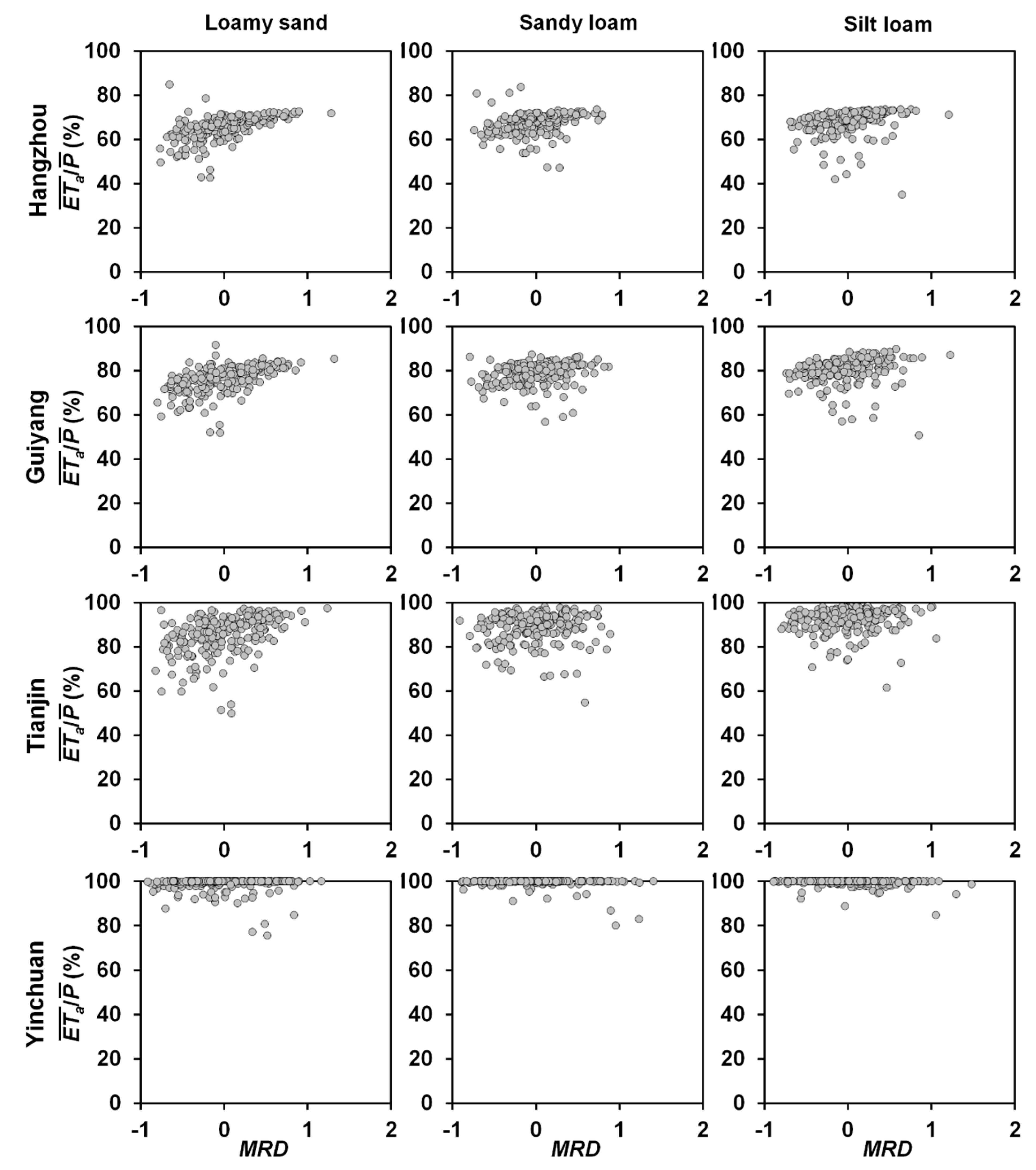
To investigate the interplays between soil moisture and flux hydrological variables across vadose zones on the basis of the TSA method, the relationships between MRD and are plotted in Figure 4 for the study sites. Note that due to the symmetry of the distributions of and (Figure 3), the relationships between MRD and are not shown here for brevity. In addition, the non-parametric Spearman’s rank correlation test was also carried out, and the correlation coefficients (rp) of MRD with and are reported in Table 4. Overall, there existed positive correlations between MRD and , while negative ones between MRD and (Table 4). The positive dependence of ETa on soil moisture levels has been widely observed in the field [12,59]. Meanwhile, finer textured soils tend to have larger water holding capacities and lower GR [31], which leads to higher soil moisture levels and MRD values for finer soils, and thus the negative correlation between MRD and GR.
More importantly, Figure 4 reveals that the ranges of MRD were similar at all sites for different soil textures; whereas, the ranges of varied substantially across the sites. Specifically, the positive correlation between MRD and was much stronger under wetter climatic conditions (e.g., Hangzhou and Guiyang) than under drier climatic conditions (e.g., Tianjin and Yinchuan; Table 4). In addition to climatic controls, soil hydraulic properties also play significant roles in affecting soil moisture levels, and thus MRD. As observed by Wang and Franz [9], the spatial distributions of MRD in Utah and the southeast United States were largely determined by soil hydraulic properties (most notably θr). Physically speaking, soil moisture levels cannot reach below θr under natural conditions. As such, regardless of climatic conditions, soil moisture levels might still vary considerably due to the variability in soil hydraulic properties (Figure 4). In contrast, as previously illustrated, the dependence of ETa on soil hydraulic properties greatly weakened under drier climatic conditions, leading to the smaller variability in for different samples (e.g., at Yinchuan). To further demonstrate the varying dependence of MRD and on soil hydraulic properties with climatic conditions, rp of MRD and with different soil hydraulic parameters was computed for sandy loam, and the results are reported in Table 5. It is clear from Table 5 that the control of θr on MRD greatly strengthened with increasing climate dryness, while the impacts of soil hydraulic properties on along the gradient of increasing climate dryness was less obvious. Therefore, owing to the differences in the dependence of MRD and on soil hydraulic properties, the correlation between MRD and varied across different climate regimes. Moreover, Table 4 shows that the correlation between MRD and was also dependent on soil texture. It appears that correlations between MRD and were stronger for coarser soils (e.g., loamy sand) under the same climatic conditions, probably due to the tighter hydrological connection between vadose zone and land surface processes.
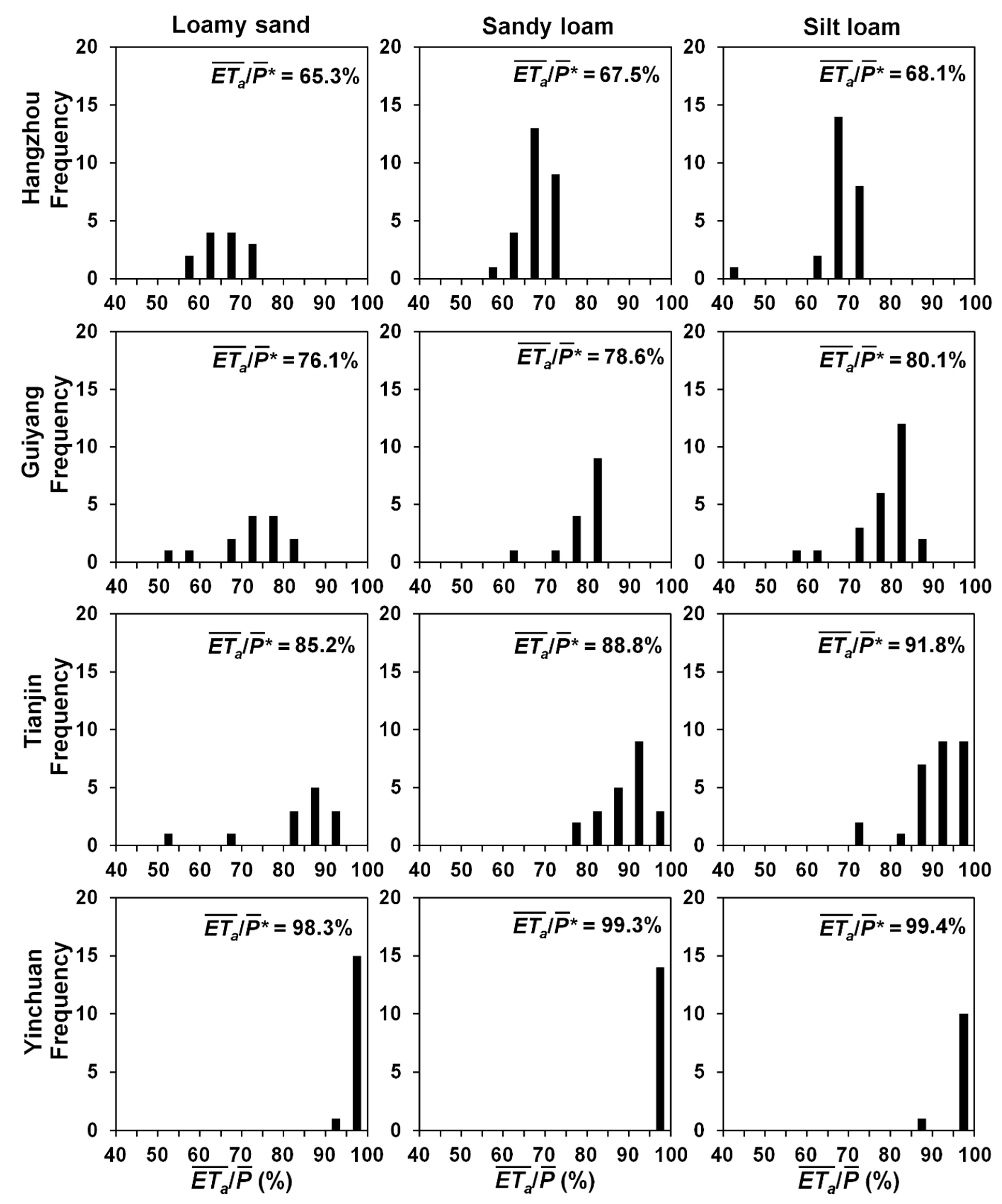
One of the main aims of the TSA method is to identify representative locations for measuring areal average moisture conditions [18]. Here, the criterion of MRD < ±0.05 was adopted to select representative samples with moisture conditions close to the average [60]. To examine whether the selected representative samples could also produce values close to the average of all samples (denoted as hereafter), histograms of associated with MRD < ±0.05 are shown in Figure 5 for different soil textures at the study sites. It can be seen from Figure 5 that the resulting number of representative samples with MRD < ±0.05 were different across the sites and for different soil textures. More importantly, although MRD only changed from −0.05 to 0.05 for the selected representative samples, associated generally exhibited much wider ranges when compared to , except for at the site of Yinchuan. Due to the arid climate at Yinchuan, the spread of associated was significantly reduced; thus, corresponded well with the majority of associated . Nevertheless, Figure 5 suggests that representative soil samples with moisture conditions close to the average as identified by the TSA method did not necessarily lead to representative soil samples for inferring , especially under wet climatic conditions.
With the aid of the TSA concept, the criterion of () < ±0.01 was used here for choosing representative samples with close to . Using the same method as above, a similar result can be obtained, which shows that in spite of the use of the narrow range of for selecting representative samples, the distributions of associated MRD with () < ±0.01 were much more scattered. It suggests that samples with average flux conditions might exhibit significant variability in soil moisture conditions.
To further reveal the correlations between average state and flux hydrological variables, an example is given in Figure 6, which shows the relationships of MRD and with different soil hydraulic parameters for sandy loam at Guiyang. In the figure, samples with MRD < ±0.05 are highlighted. Part of the reason for the loose connection between average state and flux variables can be attributed to the complex interactions of MRD and with soil hydraulic parameters, due to the high non-linearity of subsurface processes. Figure 6 shows that MRD from the representative samples was almost irrespective of θr, but associated exhibited a clear negative relationship with θr. It is clear that samples with average moisture conditions generally do not correspond with samples with average values, especially for the study sites with wet climatic conditions.
4. Conclusions
A synthetic modeling approach with generated soil hydraulic parameters was utilized in this study to investigate the interplays between state and flux hydrological variables across vadose zones in different climate zones. On the basis of the TSA method, reasonable soil moisture spatiotemporal structures were reproduced from the model. The simulation results revealed that although MRD, ETa, and GR were affected by both climate and soil, their dependence on soil hydraulic properties varied considerably with climatic conditions. In particular, the controls of soil hydraulic properties on ETa and GR greatly weakened under arid climatic conditions due to the limited water supplies, whereas the distribution of MRD still largely depended on soil hydraulic properties under the same climatic conditions. As such, the correlations of MRD with ETa and GR varied with climatic conditions. Moreover, the modeling results showed that samples with average moisture conditions did not necessarily correspond with those with average flux conditions, which resulted from the complex interactions of soil moisture, ETa, and GR with soil hydraulic properties. Although the TSA method has been widely used for selecting representative locations for monitoring areal average moisture conditions, the results of this study underscore the importance of using soil moisture information from multiple sites to infer areal average values of ETa and GR, even with the knowledge of representative soil moisture monitoring sites.
Author Contributions
Conceptualization, T.W.; formal analysis, Z.W., T.W. and Y.Z.; data curation, Z.W. and Y.Z.; writing—original draft preparation, T.W.; writing—review and editing, Z.W.
Acknowledgments
The authors would like to thank the National Centers for Environmental Information for providing the hydrometeorological data used in this study. This study was supported by the National Natural Scientific Foundation of China (U1612441) and the National Key R&D Program of China (2016 YFA0601002). The authors would like to acknowledge the financial support from the Tianjin University, and T.W. also acknowledges the financial support from the Thousand Talent Program for Young Outstanding Scientists for this study.
Conflicts of Interest
The authors declare no conflict of interest.
References
- Scanlon, B.R.; Keese, K.E.; Flint, A.L.; Flint, L.E.; Gaye, C.B.; Edmunds, W.M.; Simmers, I. Global synthesis of groundwater recharge in semiarid and arid regions. Hydrol. Process. 2006, 20, 3335–3370. [Google Scholar] [CrossRef]
- Robinson, D.A.; Campbell, C.S.; Hopmans, J.W.; Hornbuckle, B.K.; Jones, S.B.; Knight, R.; Ogden, F.; Selker, J.; Wendroth, O. Soil moisture measurement for ecological and hydrological watershed-scale observatories: A review. Vadose Zone J. 2008, 7, 358–389. [Google Scholar] [CrossRef]
- Wang, K.; Dickinson, R.E. A review of global terrestrial evapotranspiration: Observation, modeling, climatology, and climatic variability. Rev. Geophys. 2012, 50. [Google Scholar] [CrossRef]
- Seneviratne, S.I.; Corti, T.; Davin, E.L.; Hirschi, M.; Jaeger, E.B.; Lehner, I.; Orlowsky, B.; Teuling, A.J. Investigating soil moisture–climate interactions in a changing climate: A review. Earth-Sci. Rev. 2010, 99, 125–161. [Google Scholar] [CrossRef]
- Vereecken, H.; Huisman, J.A.; Pachepsky, Y.; Montzka, C.; van der Kruk, J.; Bogena, H.; Weihermüller, L.; Herbst, M.; Martinez, G.; Vanderborght, J. On the spatio-temporal dynamics of soil moisture at the field scale. J. Hydrol. 2014, 516, 76–96. [Google Scholar] [CrossRef]
- Keese, K.E.; Scanlon, B.R.; Reedy, R.C. Assessing controls on diffuse groundwater recharge using unsaturated flow modeling. Water Resour. Res. 2005, 41. [Google Scholar] [CrossRef] [Green Version]
- Szilagyi, J.; Zlotnik, V.A.; Gates, J.B.; Jozsa, J. Mapping mean annual groundwater recharge in the Nebraska Sand Hills, USA. Hydrogeol. J. 2011, 19, 1503–1513. [Google Scholar] [CrossRef] [Green Version]
- Trambauer, P.; Dutra, E.; Maskey, S.; Werner, M.; Pappenberger, F.; van Beek, L.P.H.; Uhlenbrook, S. Comparison of different evaporation estimates over the African continent. Hydrol. Earth Syst. Sci. 2014, 18, 193–212. [Google Scholar] [CrossRef] [Green Version]
- Wang, T.; Franz, T.E.; Zlotnik, V.A. Controls of soil hydraulic characteristics on modeling groundwater recharge under different climatic conditions. J. Hydrol. 2015, 521, 470–481. [Google Scholar] [CrossRef]
- Daly, E.; Porporato, A. A review of soil moisture dynamics: From rainfall infiltration to ecosystem response. Environ. Eng. Sci. 2005, 22, 9–24. [Google Scholar] [CrossRef]
- Kirchner, J.W. Getting the right answers for the right reasons: Linking measurements, analyses, and models to advance the science of hydrology. Water Resour. Res. 2006, 42. [Google Scholar] [CrossRef]
- Vivoni, E.R.; Moreno, H.A.; Mascaro, G.; Rodriguez, J.C.; Watts, C.J.; Garatuza-Payan, J.; Scott, R.L. Observed relation between evapotranspiration and soil moisture in the North American monsoon region. Geophys. Res. Lett. 2008, 35. [Google Scholar] [CrossRef] [Green Version]
- Peters-Lidard, C.D.; Clark, M.; Samaniego, L.; Verhoest, N.E.C.; van Emmerik, T.; Uijlenhoet, R.; Achieng, K.; Franz, T.E.; Woods, R. Scaling, similarity, and the fourth paradigm for hydrology. Hydrol. Earth Syst. Sci. 2017, 21, 3701–3713. [Google Scholar] [CrossRef] [PubMed] [Green Version]
- Jung, M.; Reichstein, M.; Ciais, P.; Seneviratne, S.I.; Sheffield, J.; Goulden, M.L.; Bonan, G.; Cescatti, A.; Chen, J.; de Jeu, R.; et al. Recent decline in the global land evapotranspiration trend due to limited moisture supply. Nature 2010, 467, 951. [Google Scholar] [CrossRef]
- Wang, T.; Franz, T.E.; Yue, W.; Szilagyi, J.; Zlotnik, V.A.; You, J.; Chen, X.; Shulski, M.D.; Young, A. Feasibility analysis of using inverse modeling for estimating natural groundwater recharge from a large-scale soil moisture monitoring network. J. Hydrol. 2016, 533, 250–265. [Google Scholar] [CrossRef]
- Crow, W.T.; Berg, A.A.; Cosh, M.H.; Loew, A.; Mohanty, B.P.; Panciera, R.; de Rosnay, P.; Ryu, D.; Walker, J.P. Upscaling sparse ground-based soil moisture observations for the validation of coarse-resolution satellite soil moisture products. Rev. Geophys. 2012, 50. [Google Scholar] [CrossRef] [Green Version]
- Liu, S.; Xu, Z.; Song, L.; Zhao, Q.; Ge, Y.; Xu, T.; Ma, Y.; Zhu, Z.; Jia, Z.; Zhang, F. Upscaling evapotranspiration measurements from multi-site to the satellite pixel scale over heterogeneous land surfaces. Agric. For. Meteorol. 2016, 230–231, 97–113. [Google Scholar] [CrossRef]
- Vachaud, G.; Passerat De Silans, A.; Balabanis, P.; Vauclin, M. Temporal stability of spatially measured soil water probability density function1. Soil Sci. Soc. Am. J. 1985, 49, 822–828. [Google Scholar] [CrossRef]
- Vanderlinden, K.; Vereecken, H.; Hardelauf, H.; Herbst, M.; Martínez, G.; Cosh, M.H.; Pachepsky, Y.A. Temporal stability of soil water contents: A review of data and analyses. Vadose Zone J. 2012, 11. [Google Scholar] [CrossRef]
- Pachepsky, Y.A.; Guber, A.K.; Jacques, D. Temporal persistence in vertical distributions of soil moisture contents. Soil Sci. Soc. Am. J. 2005, 69, 347–352. [Google Scholar] [CrossRef]
- Starr, G.C. Assessing temporal stability and spatial variability of soil water patterns with implications for precision water management. Agric. Water Manag. 2005, 72, 223–243. [Google Scholar] [CrossRef]
- Guber, A.K.; Gish, T.J.; Pachepsky, Y.A.; van Genuchten, M.T.; Daughtry, C.S.T.; Nicholson, T.J.; Cady, R.E. Temporal stability in soil water content patterns across agricultural fields. Catena 2008, 73, 125–133. [Google Scholar] [CrossRef]
- Brocca, L.; Melone, F.; Moramarco, T.; Morbidelli, R. Spatial-temporal variability of soil moisture and its estimation across scales. Water Resour. Res. 2010, 46. [Google Scholar] [CrossRef]
- Wang, T.; Liu, Q.; Franz, T.E.; Li, R.; Lang, Y.; Fiebrich, C.A. Spatial patterns of soil moisture from two regional monitoring networks in the United States. J. Hydrol. 2017, 552, 578–585. [Google Scholar] [CrossRef]
- Scanlon, B.R.; Healy, R.W.; Cook, P.G. Choosing appropriate techniques for quantifying groundwater recharge. Hydrogeol. J. 2002, 10, 18–39. [Google Scholar] [CrossRef]
- Turkeltaub, T.; Kurtzman, D.; Bel, G.; Dahan, O. Examination of groundwater recharge with a calibrated/validated flow model of the deep vadose zone. J. Hydrol. 2015, 522, 618–627. [Google Scholar] [CrossRef]
- Foolad, F.; Franz, T.E.; Wang, T.; Gibson, J.; Kilic, A.; Allen, R.G.; Suyker, A. Feasibility analysis of using inverse modeling for estimating field-scale evapotranspiration in maize and soybean fields from soil water content monitoring networks. Hydrol. Earth Syst. Sci. 2017, 21, 1263–1277. [Google Scholar] [CrossRef] [Green Version]
- Martínez, G.; Pachepsky, Y.A.; Vereecken, H. Temporal stability of soil water content as affected by climate and soil hydraulic properties: A simulation study. Hydrol. Process. 2014, 28, 1899–1915. [Google Scholar] [CrossRef]
- Wang, T. Modeling the impacts of soil hydraulic properties on temporal stability of soil moisture under a semi-arid climate. J. Hydrol. 2014, 519, 1214–1224. [Google Scholar] [CrossRef]
- Vereecken, H.; Kamai, T.; Harter, T.; Kasteel, R.; Hopmans, J.; Vanderborght, J. Explaining soil moisture variability as a function of mean soil moisture: A stochastic unsaturated flow perspective. Geophys. Res. Lett. 2007, 34. [Google Scholar] [CrossRef] [Green Version]
- Wang, T.; Zlotnik, V.A.; Šimunek, J.; Schaap, M.G. Using pedotransfer functions in vadose zone models for estimating groundwater recharge in semiarid regions. Water Resour. Res. 2009, 45. [Google Scholar] [CrossRef] [Green Version]
- Simunek, J.; Sejna, M.; Saito, H.; Sakai, M.; van Genuchten, M.T. The HYDRUS-1 D Software Package for Simulating the One-Dimensional Movement of Water, Heat, and Multiple Solutes in Variably-Saturated Media; Version 4.17; Depart. of Environ. Sci., University of California Riverside: Riverside, CA, USA, 2013; p. 308. [Google Scholar]
- Zlotnik, V.A.; Wang, T.; Nieber, J.L.; Šimunek, J. Verification of numerical solutions of the Richards equation using a traveling wave solution. Adv. Water Resour. 2007, 30, 1973–1980. [Google Scholar] [CrossRef]
- Neuman, S.P.; Feddes, R.A.; Bresler, E. Finite Element Simulation of Flow in Saturated-Unsaturated Soils Considering Water Uptake by Plants; Third Annual Report; Proj. A10-SWC-77; Hydraul. Eng. Lab., Technion: Haifa, Israel, 1974. [Google Scholar]
- Feddes, R.A.; Kowalik, P.J.; Neuman, S.P. Simulation of Field Water Use and Crop Yield; John Wiley and Sons: New York, NY, USA, 1978. [Google Scholar]
- Ritchie, J.T. Model for predicting evaporation from a row crop with incomplete cover. Water Resour. Res. 1972, 8, 1204–1213. [Google Scholar] [CrossRef] [Green Version]
- Wang, T.; Zlotnik, V.A. A complementary relationship between actual and potential evapotranspiration and soil effects. J. Hydrol. 2012, 456–457, 146–150. [Google Scholar] [CrossRef]
- Myneni, R.B.; Hoffman, S.; Knyazikhin, Y.; Privette, J.L.; Glassy, J.; Tian, Y.; Wang, Y.; Song, X.; Zhang, Y.; Smith, G.R.; et al. Global products of vegetation leaf area and fraction absorbed PAR from year one of MODIS data. Remote Sens. Environ. 2002, 83, 214–231. [Google Scholar] [CrossRef] [Green Version]
- Jackson, R.B.; Canadell, J.; Ehleringer, J.R.; Mooney, H.A.; Sala, O.E.; Schulze, E.D. A global analysis of root distributions for terrestrial biomes. Oecologia 1996, 108, 389–411. [Google Scholar] [CrossRef]
- Small, E.E. Climatic controls on diffuse groundwater recharge in semiarid environments of the southwestern United States. Water Resour. Res. 2005, 41. [Google Scholar] [CrossRef]
- Available online: http://www.ncdc.noaa.gov/cdo-web/ (accessed on 19 June 2019).
- Hargreaves, G.H.; Samani, Z.A. Estimation potential evapotranspiration. J. Irrig. Drain. Eng. ASCE 1982, 108, 223–230. [Google Scholar]
- Gutiérrez-Jurado, H.A.; Vivoni, E.R.; Harrison, J.B.J.; Guan, H. Ecohydrology of root zone water fluxes and soil development in complex semiarid rangelands. Hydrol. Process. 2006, 20, 3289–3316. [Google Scholar] [CrossRef]
- Vogel, T.; Dohnal, M.; Dusek, J.; Votrubova, J.; Tesar, M. Macroscopic modeling of plant water uptake in a forest stand involving root-mediated soil water redistribution. Vadose Zone J. 2013, 12. [Google Scholar] [CrossRef]
- Wesseling, J.G. Meerjarige Simulatie van Grondwaterstroming voor Verschillende Bodemprofielen, Grondwatertrappen en Gewassen Met Het Model SWATRE. Rapport 152; Wageningen, DLO-Staring Centrum. 1991, p. 63. Available online: https://library.wur.nl/WebQuery/wurpubs/fulltext/304226 (accessed on 19 June 2019).
- Mualem, Y. A new model for predicting the hydraulic conductivity of unsaturated porous media. Water Resour. Res. 1976, 12, 513–522. [Google Scholar] [CrossRef] [Green Version]
- Van Genuchten, M.T. A closed-form equation for predicting the hydraulic conductivity of unsaturated soils. Soil Sci. Soc. Am. J. 1980, 44, 892–898. [Google Scholar] [CrossRef]
- Lawrence, J.E.; Hornberger, G.M. Soil moisture variability across climate zones. Geophys. Res. Lett. 2007, 34. [Google Scholar] [CrossRef]
- Teuling, A.J.; Hupet, F.; Uijlenhoet, R.; Troch, P.A. Climate variability effects on spatial soil moisture dynamics. Geophys. Res. Lett. 2007, 34. [Google Scholar] [CrossRef]
- Zhang, Y.; Schaap, M.G. Weighted recalibration of the Rosetta pedotransfer model with improved estimates of hydraulic parameter distributions and summary statistics (Rosetta3). J. Hydrol. 2017, 547, 39–53. [Google Scholar] [CrossRef] [Green Version]
- Zhang, Y.; Schaap, M.G.; Guadagnini, A.; Neuman, S.P. Inverse modeling of unsaturated flow using clusters of soil texture and pedotransfer functions. Water Resour. Res. 2016, 52, 7631–7644. [Google Scholar] [CrossRef] [Green Version]
- Martínez-Fernández, J.; Ceballos, A. Temporal stability of soil moisture in a large-field experiment in Spain. Soil Sci. Soc. Am. J. 2003, 67, 1647–1656. [Google Scholar] [CrossRef]
- Wang, T.; Franz, T.E. Field observations of regional controls of soil hydraulic properties on soil moisture spatial variability in different climate zones. Vadose Zone J. 2015, 14. [Google Scholar] [CrossRef]
- Yokoo, Y.; Sivapalan, M.; Oki, T. Investigating the roles of climate seasonality and landscape characteristics on mean annual and monthly water balances. J. Hydrol. 2008, 357, 255–269. [Google Scholar] [CrossRef]
- Cosh, M.H.; Jackson, T.J.; Moran, S.; Bindlish, R. Temporal persistence and stability of surface soil moisture in a semi-arid watershed. Remote Sens. Environ. 2008, 112, 304–313. [Google Scholar] [CrossRef]
- Zhao, Y.; Peth, S.; Wang, X.Y.; Lin, H.; Horn, R. Controls of surface soil moisture spatial patterns and their temporal stability in a semi-arid steppe. Hydrol. Process. 2010, 24, 2507–2519. [Google Scholar] [CrossRef]
- Zhang, L.; Dawes, W.R.; Walker, G.R. Response of mean annual evapotranspiration to vegetation changes at catchment scale. Water Resour. Res. 2001, 37, 701–708. [Google Scholar] [CrossRef]
- Wang, T.; Istanbulluoglu, E.; Lenters, J.; Scott, D. On the role of groundwater and soil texture in the regional water balance: An investigation of the Nebraska Sand Hills, USA. Water Resour. Res. 2009, 45. [Google Scholar] [CrossRef] [Green Version]
- Chen, X.; Rubin, Y.; Ma, S.; Baldocchi, D. Observations and stochastic modeling of soil moisture control on evapotranspiration in a Californian oak savanna. Water Resour. Res. 2008, 44. [Google Scholar] [CrossRef]
- Hu, W.; Shao, M.; Han, F.; Reichardt, K.; Tan, J. Watershed scale temporal stability of soil water content. Geoderma 2010, 158, 181–198. [Google Scholar] [CrossRef]
Figure 1.
Mean monthly precipitation (P) and potential evapotranspiration (ETp) during the study period at (a) Hangzhou, (b) Guiyang, (c) Tianjin, and (d) Yinchuan.
Figure 1.
Mean monthly precipitation (P) and potential evapotranspiration (ETp) during the study period at (a) Hangzhou, (b) Guiyang, (c) Tianjin, and (d) Yinchuan.

Figure 2.
Ranked mean relative difference (MRD) of soil moisture with one standard deviation (vertical bars) for different soil textures at the study sites. Simulated soil moisture data at 25 cm were used to compute MRD.
Figure 2.
Ranked mean relative difference (MRD) of soil moisture with one standard deviation (vertical bars) for different soil textures at the study sites. Simulated soil moisture data at 25 cm were used to compute MRD.

Figure 3.
Distributions of simulated mean annual ratios of actual evapotranspiration () and groundwater recharge () over precipitation ().
Figure 3.
Distributions of simulated mean annual ratios of actual evapotranspiration () and groundwater recharge () over precipitation ().

Figure 4.
Relationships of mean relative difference (MRD) of soil moisture with mean annual ratio of actual evapotranspiration () over precipitation ().
Figure 4.
Relationships of mean relative difference (MRD) of soil moisture with mean annual ratio of actual evapotranspiration () over precipitation ().

Figure 5.
Distributions of mean annual ratio of actual evapotranspiration () over precipitation (). Samples with MRD < ±0.05 are used here to plot the distributions of . is the average value of from all samples.
Figure 5.
Distributions of mean annual ratio of actual evapotranspiration () over precipitation (). Samples with MRD < ±0.05 are used here to plot the distributions of . is the average value of from all samples.

Figure 6.
Relationships of MRD and with different soil hydraulic parameters for sandy loam at Guiyang. Samples with MRD < ±0.05 are highlighted in red.
Figure 6.
Relationships of MRD and with different soil hydraulic parameters for sandy loam at Guiyang. Samples with MRD < ±0.05 are highlighted in red.


Table 1.
Mean annual precipitation (), potential evapotranspiration (), and aridity index (/) at the study sites.
Table 1.
Mean annual precipitation (), potential evapotranspiration (), and aridity index (/) at the study sites.
| Location | Latitude | Longitude | (-) | ||
|---|---|---|---|---|---|
| Hangzhou | 30.23°N | 120.17°E | 150.9 (127.4–172.9) * | 111.8 (108.0–115.1) | 0.74 (0.62–0.89) |
| Guiyang | 26.58°N | 106.73°E | 103.8 (73.5–137.1) | 101.7 (95.9–104.6) | 0.98 (0.74–1.40) |
| Tianjin | 39.10°N | 117.17°E | 54.3 (35.6–75.7) | 104.1 (99.9–107.2) | 1.92 (1.37–2.81) |
| Yinchuan | 38.47°N | 106.20°E | 20.8 (16.6–29.2) | 108.6 (106.8–110.5) | 5.22 (3.74–6.43) |
* The range of annual values is given in the parentheses.
Table 2.
Average values of soil hydraulic parameters for the van Genuchten–Mualem model generated for different soil textural classes.
Table 2.
Average values of soil hydraulic parameters for the van Genuchten–Mualem model generated for different soil textural classes.
| Soil Texture | θr (cm3 cm−3) | θs (cm3 cm−3) | α (1/cm) | n (-) | Ks (cm/day) |
|---|---|---|---|---|---|
| Loamy sand | 0.064 (0.035) * | 0.386 (0.063) | 0.036 (0.039) | 1.908 (0.580) | 342.5 (864.1) |
| Sandy loam | 0.076 (0.047) | 0.381 (0.068) | 0.040 (0.075) | 1.673 (0.359) | 125.4 (334.1) |
| Silt loam | 0.098 (0.057) | 0.432 (0.077) | 0.006 (0.007) | 1.790 (0.475) | 62.8 (180.9) |
* Standard deviation values are given in parenthesis.
Table 3.
Statistical summary of mean relative difference (MRD) and standard deviation of relative difference (SDRD) of soil moisture. Simulated soil moisture data at 25 cm were used to compute MRD and SDRD.
Table 3.
Statistical summary of mean relative difference (MRD) and standard deviation of relative difference (SDRD) of soil moisture. Simulated soil moisture data at 25 cm were used to compute MRD and SDRD.
| Location | Loamy Sand | Sandy Loam | Silt Loam | ||||||
|---|---|---|---|---|---|---|---|---|---|
| Range of MRD | Range of SDRD | Mean SDRD | Range of MRD | Range of SDRD | Mean SDRD | Range of MRD | Range of SDRD | Mean SDRD | |
| Hangzhou | −0.765–1.287 | 0.046–0.428 | 0.139 | −0.741–0.799 | 0.041–0.402 | 0.131 | −0.690–1.210 | 0.022–0.264 | 0.085 |
| Guiyang | −0.797–1.324 | 0.037–0.486 | 0.158 | −0.789–0.873 | 0.049–0.430 | 0.159 | −0.732–1.230 | 0.027–0.370 | 0.112 |
| Tianjin | −0.819–1.237 | 0.043–0.462 | 0.133 | −0.977–0.891 | 0.053–0.397 | 0.134 | −0.793–1.064 | 0.032–0.301 | 0.091 |
| Yinchuan | −0.912–1.166 | 0.035–0.397 | 0.114 | −0.889–1.410 | 0.043–0.664 | 0.111 | −0.890–1.485 | 0.024–0.199 | 0.073 |
Table 4.
Spearman’s rank correlation coefficients of mean relative difference (MRD) of soil moisture with mean annual ratios of actual evapotranspiration () and groundwater recharge () over precipitation ().
Table 4.
Spearman’s rank correlation coefficients of mean relative difference (MRD) of soil moisture with mean annual ratios of actual evapotranspiration () and groundwater recharge () over precipitation ().
| Location | Loamy Sand | Sandy Loam | Silt Loam | |||
|---|---|---|---|---|---|---|
| Hangzhou | 0.679 | −0.668 | 0.431 | −0.429 | 0.461 | −0.462 |
| Guiyang | 0.630 | −0.623 | 0.288 | −0.279 | 0.378 | −0.393 |
| Tianjin | 0.482 | −0.478 | 0.123 | −0.145 * | 0.188 ** | −0.258 |
| Yinchuan | 0.255 | −0.297 | 0.227 ** | −0.241 | 0.089 | −0.158 * |
* p < 0.05; ** p < 0.01; values in bold with p < 0.001.
Table 5.
Spearman’s rank correlation coefficients of soil hydraulic parameters for sandy loam with mean relative difference (MRD) of soil moisture and mean annual ratio of actual evapotranspiration () over precipitation ().
Table 5.
Spearman’s rank correlation coefficients of soil hydraulic parameters for sandy loam with mean relative difference (MRD) of soil moisture and mean annual ratio of actual evapotranspiration () over precipitation ().
| Soil Hydraulic Parameters | Hangzhou | Guiyang | Tianjin | Yinchuan | ||||
|---|---|---|---|---|---|---|---|---|
| MRD | MRD | MRD | MRD | |||||
| θr | 0.411 | −0.372 | 0.573 | −0.369 | 0.734 | −0.356 | 0.920 | −0.018 |
| θs | 0.497 | 0.481 | 0.398 | 0.422 | 0.219 ** | 0.351 | 0.026 | −0.095 |
| α | −0.012 | −0.176 * | 0.026 | −0.307 | 0.038 | −0.443 | 0.061 | −0.493 |
| n | −0.568 | −0.270 | −0.578 | −0.351 | −0.548 | −0.363 | −0.294 | −0.156 * |
| Ks | −0.357 | −0.406 | −0.263 | −0.301 | −0.109 | −0.172 * | 0.008 | 0.286 |
* p < 0.05; ** p < 0.01; values in bold with p < 0.001.
© 2019 by the authors. Licensee MDPI, Basel, Switzerland. This article is an open access article distributed under the terms and conditions of the Creative Commons Attribution (CC BY) license (http://creativecommons.org/licenses/by/4.0/).
Share and Cite
MDPI and ACS Style
Wang, Z.; Wang, T.; Zhang, Y. Interplays between State and Flux Hydrological Variables across Vadose Zones: A Numerical Investigation. Water 2019, 11, 1295. https://doi.org/10.3390/w11061295
AMA Style
Wang Z, Wang T, Zhang Y. Interplays between State and Flux Hydrological Variables across Vadose Zones: A Numerical Investigation. Water. 2019; 11(6):1295. https://doi.org/10.3390/w11061295
Chicago/Turabian StyleWang, Zhaoxin, Tiejun Wang, and Yonggen Zhang. 2019. "Interplays between State and Flux Hydrological Variables across Vadose Zones: A Numerical Investigation" Water 11, no. 6: 1295. https://doi.org/10.3390/w11061295
Note that from the first issue of 2016, this journal uses article numbers instead of page numbers. See further details here.