A 60-Year Time Series Analyses of the Upwelling along the Portuguese Coast

Abstract

Coastal upwelling has a significant local impact on marine coastal environment and on marine biology, namely fisheries. This study aims to evaluate climate and environmental changes in upwelling trends between 1950 and 2010. Annual, seasonal and monthly upwelling trends were studied in three different oceanographic areas of the Portuguese coast (northwestern—NW, southwestern—SW, and south—S). Two sea surface temperature datasets, remote sensing (RS: 1985–2009) and International Comprehensive Ocean—Atmosphere Data Set (ICOADS: 1950–2010), were used to estimate an upwelling index (UPWI) based on the difference between offshore and coastal sea surface temperature. Time series analyses reveal similar yearly and monthly trends between datasets A decrease of the UPWI was observed, extending longer than 20 years in the NW (1956–1979) and SW (1956–1994), and 30 years in the S (1956–1994). Analyses of sudden shifts reveal long term weakening and intensification periods of up to 30 years. This means that in the past 60 years a normal climate UPWI occurred along the Portuguese coast. An intensification of UPWI was recorded in recent decades regardless of the areas (RS: 1985–2009). Such an intensification rate (linear increase in UPWI) is only significant in S in recent decades (increase rate: ICOADS = 0.02 °C decade-1; RS = 0.11 °C decade-1) while in NW and SW the increase rate is meaningless. In NW more stable UPWI conditions were recorded, however average UPWI values increased in autumn and winter in NW in recently decades (RS: 1985–2009). An intensification rate of UPWI was recorded during summer (July, August and September) in SW and S in latter decades (RS: 1985–2009). The average UPWI values increased in recent decades in autumn in S. Marked phenological changes were observed in S in summer (before downwelling conditions prevail whilst recently when UPWI regimes prevail) with UPWI seasonal regime in S in recent decades becoming similar to those found in SW and NW. Results of this work can contribute to a better understanding of how upwelling dynamics affect/are correlated with biological data.

1. Introduction

Coastal upwelling regions are rich in nutrients and essential for the trophic chain of coastal fish species. About 20% of the worldwide fish catchment is captured in coastal upwelling regions [1], although upwelling areas enclose less than 1% of the world’s oceans. Populations of small pelagic fishes, such as sardine, horse mackerel, mackerel and anchovy, show evidence of significant long-term natural fluctuations in their abundance due to upwelling, which has implications for medium and long-term forecasting of catches [2,3,4]. Therefore, upwelling systems are among the most studied in the ocean due to their high productivity, intense fisheries activity and consequent economic and social implications [3,4].

The Portuguese coast is a very complex ecosystem as far as the upwelling regime is concerned [5] proposed that the Iberian Margin could be divided into different upwelling regions, each showing a different upwelling pattern related to characteristic topographical constraints. [5,6] documented the presence of a complex mesoscale activity along the Portuguese coast that generates distinct upwelling structures in different spatial scales. [5,7] recognized the necessity of specific wind regimes to generate coastal upwelling along the Iberian Margin only due to its orientation: northerly winds produce upwelling off the western coast whereas westerly winds drive it off the southern coast. The main oceanographic features referred to in the literature for the Iberian Portuguese coast are the Iberian Poleward Current (IPC), the upwelling jet and associated features like upwelling filaments and eddies and the Western Iberia Buoyant Plume [8]. According to the first climatological analyses using wind and sea surface temperature (SST) datasets for periods before 1970, maximum coastal upwelling occurs in the peak summer months (July to September), and minimum in winter [9,10]. After the 1970s several changes in this pattern were reported [2] namely a delay in the peak of intensity of the upwelling-favourable winds [11,12]. At the same time, some authors found an increasing trend in upwelling intensity [11,13], but others reported a decreasing trend [14,15]. Therefore, these changes in upwelling intensity during spring/summer need to be investigated.

The pioneering work of [13] states that an intensification of coastal upwelling as a result of the strengthening of the alongshore wind induced by an increased land-ocean pressure gradient related to the global climate change. Subsequent investigations have reached contradictory results about the temporal fluctuations of the upwelling in Iberian Peninsula. Based on measured coastal winds, [16] 2004) concluded that the upwelling index off the western Iberia coast weakened from the 1940s to the 2000s. Later, based on a statistical model, this result was confirmed by [17]. Based on spatial averages of satellite-derived SST, [17] found that the upwelling variability pattern is better described as a decadal scale shift of upwelling regime intensity from weak upwelling in the 1980s to a stronger one in the 1990s. A summary of these opposed results is given in [18]. This controversy is depicted in [14] who argued that there was no evidence of upwelling intensity off the Iberian coast. [19] studied the response of Iberian upwelling to atmospheric forcing in a regional climate scenario. Latter authors assumed that the process is not easily reproduced by current large-scale coupled models due to its coarse resolution [20] and its simulation still carries difficulties, in particular, in places characterized by frequent on–off switching of upwelling and by complex coastal circulations.

Observations of upwelling, or coastal wind responsible for its establishment, indicate that it can show significant inter-annual variability, with indications of recent systematic changes possibly in response to global warming. The western Iberia system behavior was also associated with the North Atlantic Oscillation [21]. [6,22] showed the presence in the Western Iberia ecosystem of different mesoscale upwelling structures that respond in different ways to the observed ocean warming, superimposed on the larger scale variability, as being the primary factor controlling the ecosystem functioning in the region. A complex structure of interleaved alongshore slope, shelf and coastal currents that interact with eddies, buoyant plumes, upwelling filaments and fronts, surface layer expressions of the subsurface circulation and internal waves is revealed by the latest research of [6,22].

This time-series study will allow us to evaluate climate and environmental changes in upwelling trends. Therefore, results can contribute to fisheries oceanography field by allowing to understand how regional upwelling dynamics affect/correlated with fisheries data or biological oceanographic features. This work uses two datasets to analyze yearly, monthly and seasonal upwelling time series in three different areas of the Iberian Portuguese coast. The datasets included satellite Remote Sensing (RS: from 1985 to 2009) and a longer time series of “in situ” observations, International Comprehensive Ocean—Atmosphere Data Set (ICOADS: 1950 to 2010) that were compared for: (i) assess patterns among time series among datasets; (ii) assess differences in time series among geographic areas. A multi-model time-series analyses approach was employed to assess variation and sudden shifts in upwelling trends.

2. Material and Methods

2.1. Study Area

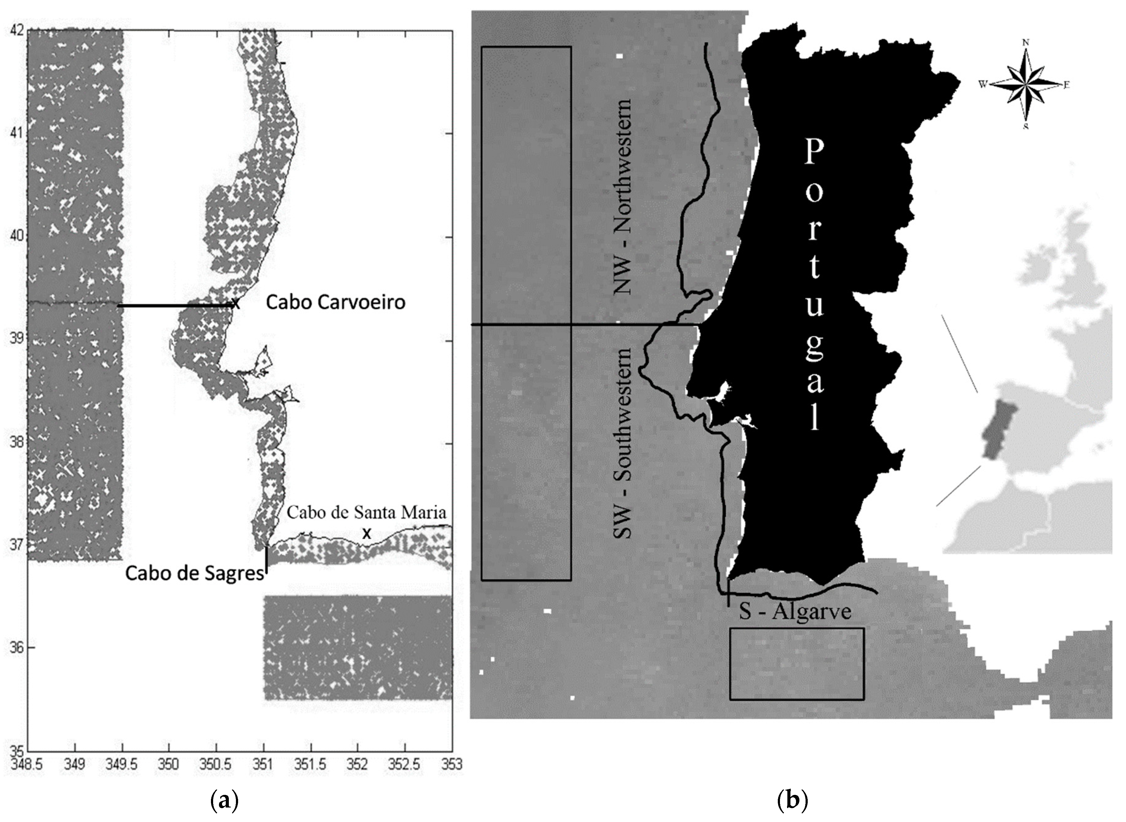
The Portuguese Iberian region covers the northern segment of the Canary Current Upwelling System (CCUS) from 42° N to 35° N and from 15° W to 7° W. For studying upwelling trends the coast was divided into three different oceanographic areas. The geographical division in areas was based on the classification of the typology of the water masses in Portugal [23] that include exposure, tidal regime, SST descriptors (Figure 1): first area from Minho at 42° N to Cabo Carvoeiro at 39°21′32″ N (called hereafter the Northwestern coast—NW), second area from Cabo Carvoeiro to Sagres at 36°59′35″ (called hereafter the Southwestern coast—SW) and the third area in the Algarve coastal zone from Sagres at 8°56′54″ W to Vila Real de Santo António at 6° W (called hereafter the South Algarve coast—S). We develop this upwelling study with future intention of relating upwelling results to fisheries biological data sets (sub-stocks). Thus, we also take into consideration the division of the coast based on ICES fishing areas IXa sub-divisions (IXa-Northwestern; IXa-Southwestern and IXa-South) that generally match the Portuguese water masses oceanographic divisions [2,23,24].

2.2. Oceanographic Data

Monthly data from international databases available through the Internet included: (i) in situ data from ICOADS Data Set Release 2.5 (http://rda.ucar.edu/datasets/ds540.0/#!imma_subset.php; [25]). The format of the ICOADS data output is ASCII text with data in fixed width columns; (ii) RS data obtained from the 4 km Advanced Very High Resolution Radiometer (AVHRR)/NOAA satellites Pathfinder Version 5 from the Physical Oceanography Distributed Active Archive Center (PO.DAAC) at NASA’s Jet Propulsion Laboratory (JPL) (ftp://podaac-ftp.jpl.nasa.gov/allData/avhrr/L3/) [26]. The RS data output is stored in the Hierarchical Data Format-Scientific Data Set (HDF-SDS).

The ICOADS is a global ocean marine meteorological and surface ocean dataset formed by measurements and visual observations from ships (merchant, navy, research), moored and drifting buoys, coastal stations, and other marine platforms. ICOADS SST observations, collected off the Iberian Peninsula, are available for the last 60 years (Figure 1b). In the case of the ICOADS, requested data included the enhanced filter options that allow the exclusion of outliers that fall outside 4.5 (broader limits) standard deviations from the smoothed median. The spatial and temporal resolution of the RS dataset is respectively of 0.044° (Latitude) × 0.044° (Longitude) and one month (monthly averaged SST observations) over 25 years from 1985 to 2009. RS data monthly SST records included only quality flags of 8 or higher. RS and ICOADS monthly SST records were spatially averaged by areas according to the boxes defined in Figure 1. The coastal areas were defined between the coastline and the 200 m isobaths, assumed as the shelf break and the outer limit of the upwelled water. Two datasets were used complementarily to assess if time-series among databases have the same trend (rather than to compare values per se) thus enhancing the confidence regarding upwelling index trends found across time. The coastal data (Figure 1) encompass waters until the 200 m isobath, the depth assumed for the continental shelf break, under upwelling influence.

2.3. Definition of the Upwelling Index

The Upwelling Index (UPWI), for both data sets (ICOADS and RS), was obtained by subtracting the offshore (control area) from the coastal average monthly SST, resulting in one single upwelling time series for each area: northwestern, southwestern and south-Algarve (subsequently referred to in this paper as NW, SW, S). If we assume that the surface expression of the upwelling is a proxy of its intensity, the former index allows us to observe the intensification (upward trend) or relaxation (downward trend) of the coastal upwelling regime. This index is positive when costal upwelling occurs, driven by favourable winds. Negative values of the index indicate upwelling absence or downwelling conditions.

The choice of an upwelling index is somewhat arbitrary and highly dependent of the research targets and available data. Routinely, upwelling indexes rely in coastal-offshore SST differences or in estimations of the Ekman transport [2,5,9,13,27,28]. Both approaches present vulnerabilities, such us the non-consideration of the subsurface structure (stratification) of the coastal region that largely modulates the upwelling efficiency. The long SST time series available and the indirect nature of the Ekman transport estimations that rely in the geostrophic wind approximation, make the first approach more appropriate to investigate the long term decadal and climatic variability. At these long time scales, the short time variability, more vulnerable to the UPWI limitations, are eliminated. The time series are smoothed and retain only the long term trends. This is the reason for their wide use [17,29,30]. The offshore ocean area free from SST upwelling variability was selected as a control area (Figure 1). The control areas for NW and SW area were distanced 2 degrees west of Cabo Carvoeiro (39°21′32″ N; 9°24′32″). Upwelling is mainly a continental shelf process, with the exception of the upwelling filaments and meanders that may occasionally stretch well beyond the shelf break. However, based on the acquired knowledge of the west coast upwelling patterns, this distance is out of the influence of such features [2,27]. The south coast control area was distanced only 1° from the south coast tip Cabo de Santa Maria at, 36°57′42″ N; 7°53′17″ W, to minimize the meridional climatological SST gradient. In S we have reduce the distance from the coast because in the south coast the shelf is narrower than in most of the western coast and it is free from long seaward upwelling front protrusions, characteristics of the western coast (upwelling filaments and meanders).

The yearly, monthly and seasonal variability off the UPWI per area for both data sets were also assessed. Some monthly observations miss from the ICOADS dataset. In these cases, the mean SST, estimated from the same months of the previous and the following years, was used to fill the gap. After 2002, the monthly SST coastal values for the S area are sparse, which could affect the yearly mean. All the analysis of the yearly UPWI long-term time series (ICOADS) for this area comprise only the period 1950–2001. Also, to assess intra-yearly variability in seasonal UPWI trends, monthly data were grouped as follows: (1) winter (January to March); (2) spring (April to June); (3) summer (July to September); and (4) autumn (October to December). Half a decade averages of the UPWI time series were also estimated to infer the inter-decadal variability of the upwelling regime in the different areas.

While it is reasonable to construct an upwelling index on the basis of nearshore-offshore SST differences, it is extremely important to first analyze the offshore SST variability on its own. Exploratory analyses of annual inshore and offshore SST were conducted (Appendix A). ICOADAS data and time series analyses techniques (see below Dynamic Factorial Analyses) showed that one common trend is enough to describe SST inshore and offshore time series across areas. Therefore, this means the inshore and offshore time series have the same trend between 1960–2010 and that the background warming trend is similar within regions for inshore and offshore time series (see also Figure A1 in Appendix A)

2.4. Time Series Analysis

A preliminary analysis of stationarity was based on the graphs of the yearly and monthly detrended observed time series, as well as by the auto-correlation function (ACF) analysis and Partial auto-correlation Function (PACF). Subsequent analyses were conducted with the software package Brodgar 2.5.1 (http://www.brodgar.com), which relates the correlation of time observations separated by different time periods [31]. Both the long-term and short-term monthly UPWI time series have a seasonal pattern. Therefore, Seasonal Decomposition by Loess (SDL) was used to detrend and smooth monthly data (Brodgar 2.5.1).

The Dynamic Factor Analysis (DFA) was used to evaluate the similarity of yearly and monthly (after LOESS transformation) UPWI time series among databases and areas. The DFA is a multivariate technique for non-stationary data that allows assessing if multiple time series (ICOADS and RS regional data) have the same trend, if different time series are related to DFA estimated common trend then they have the same trend [32,33,34]. The method used in this work was the DFA multiple (M) common trend model approach plus noise (data = M common trend + noise). However, the time series for DFA analyses (results provided in Appendix B) included solely years when both ICOADS and RS data matches among data sources, these were: (i) for ICOADS: 1985–2010 for both NW and SW and 1985–2001 for S; (ii) for RS: 1985–2009.

The time series data (yearly and monthly) were standardised before DFA analyses, that is all variables centered on zero and then divided by the sample standard deviation, resulting in unit variance and unit-less (normalisation), as advised by [32,33,34] for DFA analyses. Various DFA analyses were made using the yearly means extracted from the smoothed monthly ICOADS and RS data. These were: (i) similarity in time series within areas among databases, (ii) similarity in time series for each data base among areas. The criterion for identifying the best number of common trends to describe all-time series was based on the comparison of the Akaike Information Criterion (AIC-the lowest the AICs the better the model fitness) and by assessing the model fitness performance (Model fit and residual graphical analyses) [32]. DFA also requires the quantification of the canonical coefficients that are correlations between the original time-series and the common trends. A high canonical correlation (>0.5) indicates that the corresponding time series follows the pattern of the common trend.

A linear regression model was fitted to yearly UPWI time series. The slope parameter of the regression model was used as a proxy of the trend tendency (upward or downward) and to quantify the rate of change in time series data. The statistical significance of the linear model was assessed via a student-t test (p-value < 0.01). The null hypothesis was formulated as no trend that describes an unchanging UPWI.

2.5. Sudden Changes (Yearly and Monthly Data)

For sudden change analyses the long-term (ICOADS) datasets was used. Regime shifts are defined as rapid reorganizations of oceanographic conditions from one relatively stable state to another. In the marine environment, regimes may last for several decades and shifts often appear to be associated with changes in the climate system. There are several methods designed to detect regime shifts in both the individual time series and entire systems [35]. The overwhelming majority of these methods, however, experience deterioration in their performance toward the ends of time series [36] developed a method based on a sequential t-test that can indicate a possibility of a regime shift in real time. Herein, discontinuities in the yearly time series were detected using the Regime Shift Analyses Index—RSI [35,37] using a National Oceanic and Atmospheric Administration software application (http://www.beringclimate.noaa.gov/regimes/).

One tool that can detect the regime shifts in monthly data is the Kolmogorov-Zurbenko Adaptive (KZA) Filter [38]. This filter is available in two R packages: the kzft, Kolmogorov–Zurbenko Fourier transform and application [39] and the kza, Kolmogorov–Zurbenko adaptive algorithm for the image detection [40]. The KZ and KZA filters analyses were conducted with R-software 3.0.2 (“kza” and “kzft” packages). They both run in the RStudio program and use an interactive moving average that adjusts the length of the window according to the rate of change of the process and performs different tasks when monthly data is used: remove noise and seasonality, separate low frequency components from the original signal.

The Rodionov algorithm [35,37] was used to detect sudden changes in yearly UPW data. The Kolmogorov-Zurbenko (KZ) filter and the Kolmogorov-Zurbenko Adaptive (KZA) filter [38,41] were used to identify shifts in monthly records.

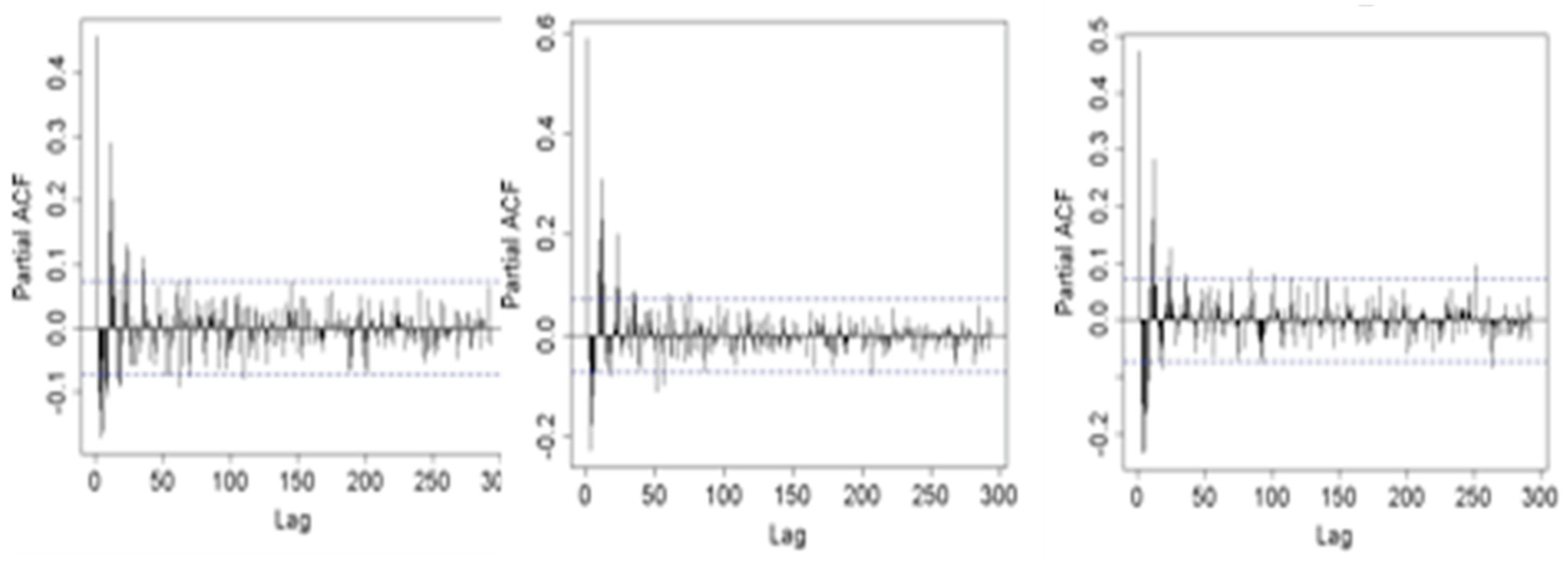
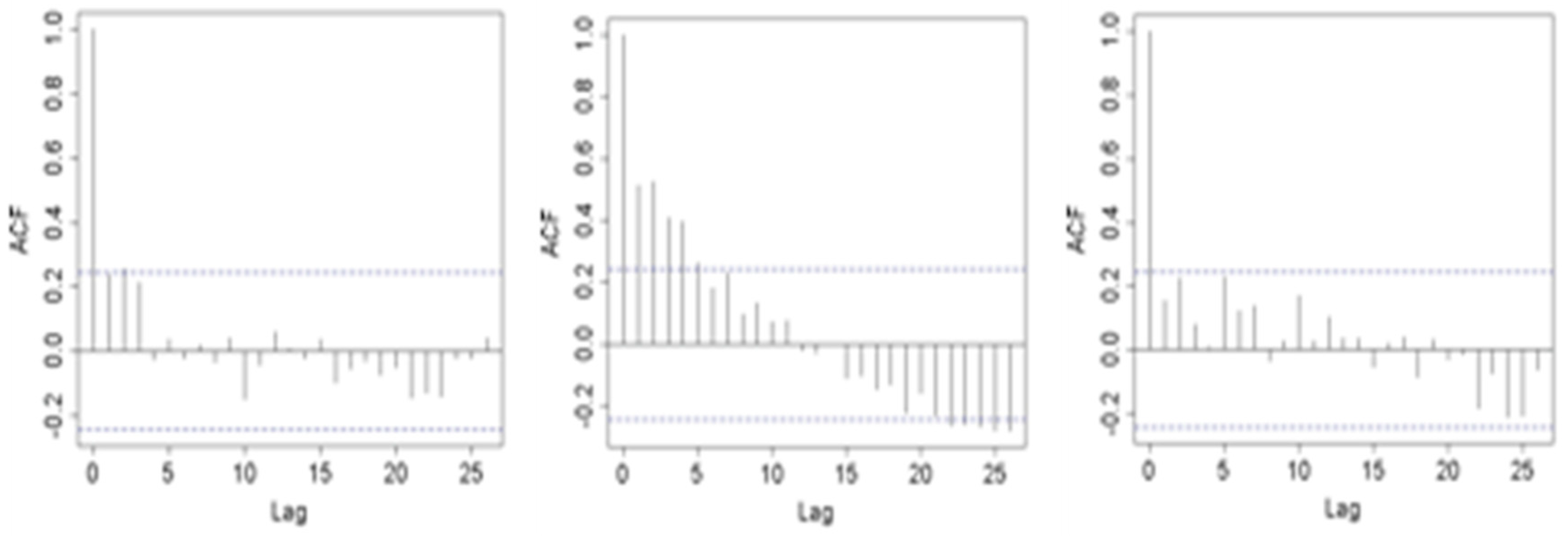
Assuming that both datasets have a common trend, the longer time-series was chosen to conduct the sudden shifts analyses (yearly and monthly). The ACF analysis was applied to the long-term UPW (ICOADS: 1950–2010) time series as a similarity between observations as a function of the time lag between them is useful for selection of the smooth and time windows components required to be modelled/applied in the Regime Shift Indicator test and KZ and KZA filters. After re-testing several models with different smooth/window sizes and considering the ACF, a lag of 3 years, 4 years and 2 years (size of the window) were used for the Northwestern, Southwestern and Southern coasts, respectively (Appendix C).

3. Results

Results achieved by the DFA of LOESS-monthly (Figure 2) and yearly (Figure 3) data show that time-series between databases within each area are described by a single common trend. That means that the different time series are similar (Appendix B:

Table A3. DFA results for evaluation of the trends among areas in each datasets (ICOADS and RS) for the monthly UPW mean values with a symmetrical matrix (see Figure 2). If the canonical correlation values (numeric value provided in table to each time-series) are higher or lower than 0.5 in absolute value than the time series correlate significantly with the common trend. The AICs value of the best model fit is provided in table, in this case the best model (lowest AICs) was for 1—common trend.

Sea Area	ICOADS	RS
	1 Trend	1 Trend
Northwestern	0.810	0.944
Southwestern	0.833	1.000
South-Algarve	−0.670	0.540
AIC Values	53.8	11.3

,

Table A4. DFA results for evaluation of the trends among datasets (ICOADS and RS) in each area for the monthly UPW mean values with a diagonal matrix model (see Figure 2). If the canonical correlation values (numeric value provided in table to each time-series) are higher or lower than 0.5 in absolute value than the time series correlate significantly with the common trend. The AICs value of the best model fit is provided in table, in this case the best model (lowest AICs) was for 1—common trend.

	Northwestern	Southwestern	South-Algarve
	1 Trend	1 Trend	1 Trend
ICOADS	0.975	0.95	1
RS	1	1	−0.682
AIC Values	12.1	11.3	28.4

,

Table A5. DFA results for evaluation of the trends among areas in each datasets (ICOADS and RS) for the annual UPW mean values with a diagonal matrix model (see Figure 4). If the canonical correlation values (numeric value provided in table to each time-series) are higher or lower than 0.5 in absolute value than the time series correlate significantly with the common trend. The AICs value of the best model fit is provided in table, in this case the best model (lowest AICs) was for 1—common trend.

	ICOADS		RS
	1 Trend	2 Trend	1 Trend
Northwestern	−0.758	0.174	0.669
Southwestern	0.414	0.649	0.983
South-Algarve	−0.402	0.853	0.891
AIC Values	210.2		191.1

,

Table A6. DFA results for evaluation of the trends among datasets (ICOADS and RS) in each area for the annual UPW mean values with a diagonal matrix model (see Figure 4). If the canonical correlation values (numeric value provided in table to each time-series) are higher or lower than 0.5 in absolute value than the time series correlate significantly with the common trend. The AICs value of the best model fit is provided in table, in this case the best model (lowest AICs) was for 1—common trend.

	Northwestern	Southwestern	South-Algarve
	1 Trend	1 Trend	1 Trend
ICOADS	0.952	0.89	0.826
RS	0.603	0.718	0.497
AIC Values	148.8	142.6	141.8

,

Table A7. DFA results for evaluation of the trends among areas in each datasets (ICOADS and RS) for the annual UPW slopes of the linear regression with a diagonal matrix model (see Figure 5). If the canonical correlation values (numeric value provided in table to each time-series) are higher or lower than 0.5 in absolute value than the time series correlate significantly with the common trend. The AICs value of the best model fit is provided in table, in this case the best model (lowest AICs) was for 1—common trend.

	ICOADS	RS
	1 Trend	1 Trend
Northwestern	−0.637	0.736
Southwestern	0.855	1.000
Southern	0.804	0.766
AIC Values	107.5	98.9

and

Table A8. DFA results for evaluation of the trends among datasets (ICOADS and RS) in each area for the annual UPW slopes of the linear regression with a diagonal matrix model (see Figure 5). If the canonical correlation values (numeric value provided in table to each time-series) are higher or lower than 0.5 in absolute value than the time series correlate significantly with the common trend. The AICs value of the best model fit is provided in table, in this case the best model (lowest AICs) was for 1—common trend.

	Northwestern	Southwestern	South-Algarve
	1 Trend	1 Trend	1 Trend
ICOADS	0.775	0.0974	−0.46
RS	1	0.924	0.905
AIC Values	70.1	63.4	78.8

). For RS yearly data, DFA showed that a single trend described all regions while for ICOADS yearly data two DFA common trends were necessary to describe all areas (1st trend—NW, and 2nd trend—SW and S areas) (Appendix B: Table A3, Table A4, Table A5 and Table A6).

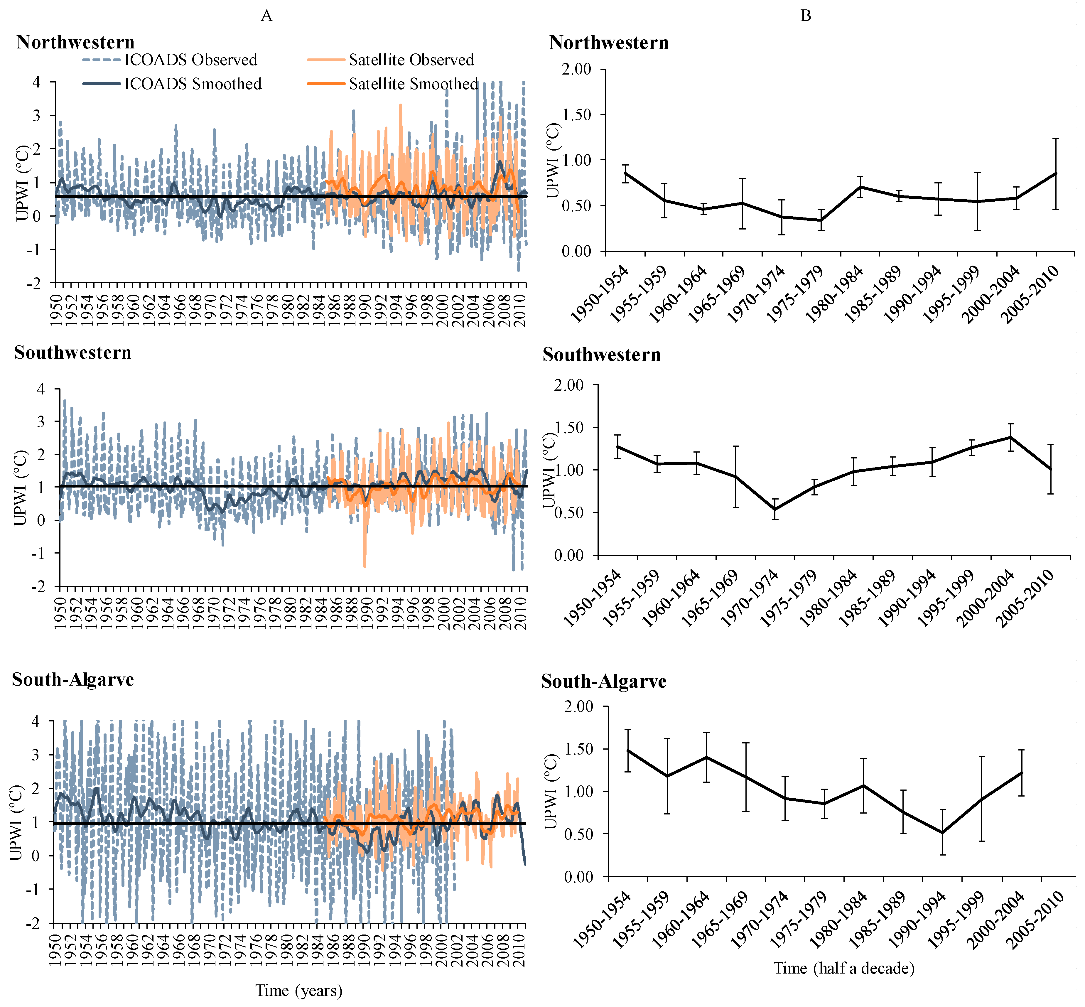
The observed monthly UPWI time series show a large variability (Figure 2, Table 2). Overall, observed and smoothed (LSD) UPWI monthly values together with the half a decade averages (

Table 1. Long-term time series (ICOADS: 1950–2010 for NW and SW and 1950–2001 for S) half decade annual UPWI mean (± standard deviation), minimum (Min) and maximum (Max) values (Celsius degrees-°C) observed (see Figure 2).

Years		Northwestern			Southwestern			S-Algarve
	Mean	Max	Min	Mean	Max	Min	Mean	Max	Min
1950−1954	0.85 (±0.10)	1.02	0.74	1.27 (±0.14)	1.40	1.08	1.48 (±0.25)	1.71	1.09
1955−1959	0.55 (±0.19)	0.81	0.28	1.07 (±0.10)	1.16	0.90	1.18 (±0.44)	1.93	0.88
1960−1964	0.46 (±0.06)	0.54	0.40	1.08 (±0.13)	1.22	0.88	1.40 (±0.29)	1.73	0.96
1965−1969	0.52 (±0.28)	0.91	0.11	0.92 (±0.36)	1.21	0.31	1.17 (±0.40)	1.66	0.58
1970−1974	0.37 (±0.19)	0.55	0.09	0.54 (±0.12)	0.66	0.39	0.92 (±0.26)	1.22	0.51
1975−1979	0.34 (±0.12)	0.52	0.21	0.80 (±0.09)	0.96	0.73	0.86 (±0.17)	1.11	0.68
1980−1984	0.70 (±0.11)	0.85	0.58	0.98 (±0.16)	1.20	0.79	1.07 (±0.32)	1.48	0.72
1985−1989	0.60 (±0.06)	0.66	0.51	1.04 (±0.11)	1.16	0.86	0.76 (±0.26)	0.96	0.32
1990−1994	0.57 (±0.18)	0.80	0.38	1.09 (±0.17)	1.38	0.93	0.52 (±0.27)	0.81	0.22
1995−1999	0.54 (±0.32)	0.98	0.14	1.26 (±0.09)	1.35	1.12	0.91 (±0.50)	1.41	0.20
2000−2004	0.58 (±0.12)	0.74	0.46	1.38 (±0.16)	1.54	1.13	1.22 (±0.27)	1.68	1.02
2005−2010	0.85 (±0.39)	1.60	0.57	1.01 (±0.29)	1.39	0.68	-	-	-

and

Table 2. Long-term (ICOADS: (1950–2010 for NW and SW and 1950–2001 for S) and short-term time series (RS: 1985-2009) monthly UPWI mean values (Celsius degrees—C°) in Northwestern (NW), Southwestern (SW) and South-Algarve (S) (see Figure 3). SD—standard deviation.

Month	ICOADS			RS
	NW	SW	S	NW	SW	S
January	0.19 ± 0.49	0.35 ± 0.77	0.35 ± 0.77	0.51 ± 0.48	1.11 ± 0.36	1.11 ± 0.36
February	0.14 ± 0.61	0.85 ± 1.17	0.85 ± 1.17	0.46 ± 0.5	1.03 ± 0.35	1.03 ± 0.35
March	0.11 ± 0.55	1.23 ± 0.83	1.23 ± 0.83	0.32 ± 0.45	0.96 ± 0.32	0.96 ± 0.32
April	0.03 ± 0.65	1.72 ± 0.84	1.72 ± 0.84	0.26 ± 0.47	0.95 ± 0.37	0.95 ± 0.37
May	0.01 ± 0.49	2.67 ± 0.94	2.67 ± 0.94	0.25 ± 0.59	1.16 ± 0.41	1.16 ± 0.41
June	0.18 ± 0.66	2.61 ± 1.15	2.61 ± 1.15	0.24 ± 0.67	0.94 ± 0.67	0.94 ± 0.67
July	0.95 ± 0.8	2.21 ± 1.3	2.21 ± 1.3	1.18 ± 0.57	0.88 ± 0.87	0.88 ± 0.87
August	1.81 ± 0.93	2 ± 1.55	2 ± 1.55	1.8 ± 0.5	1.05 ± 0.7	1.05 ± 0.7
September	1.6 ± 0.82	0.32 ± 1.58	0.32 ± 1.58	1.88 ± 0.6	1.31 ± 0.6	1.31 ± 0.6
October	1.03 ± 0.69	−0.55 ± 1.47	−0.55 ± 1.47	1.61 ± 0.71	1.61 ± 0.73	1.61 ± 0.73
November	0.61 ± 0.74	−0.35 ± 0.98	−0.35 ± 0.98	1.02 ± 0.82	1.33 ± 0.62	1.33 ± 0.62
December	0.34 ± 0.66	−0.5 ± 0.81	−0.5 ± 0.8	0.7 ± 0.52	0.77 ± 0.51	1.09 ± 0.52

) of the UPWI showed that:

(i)

all the areas show the highest UPWI values in the 50s;

(ii)

the UPWI values are higher in S, which means that the thermal gradient between offshore and coastal waters is higher there. Moreover, the UPWI standard deviations are higher in this area;

(iii)

overall UPWI generally decrease until mid 70’s in SW area, late 70s in NW area and mid 90s in S area;

(iv)

in the NW and SW UPWI increases since the 1980 and 2005;

(v)

in the S contrary to both NW and SW, the UPWI generally decreased along the entire time-series until 1995, increasing afterwards;

(vi)

half a decade averages of the UPW are positive, which indicates predominance of upwelling regime;

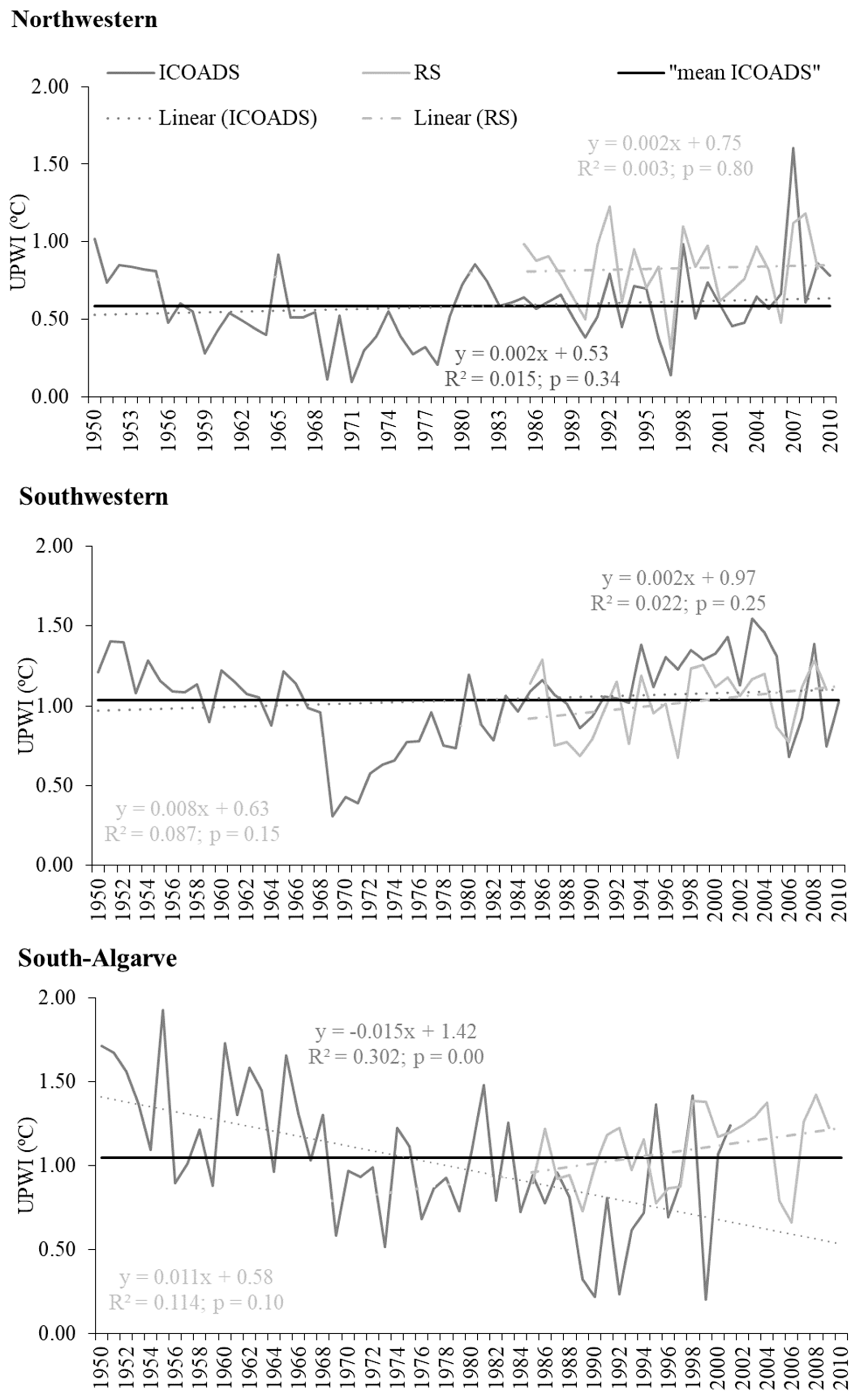
The long-term (ICOADS: 1950–2010) yearly linear UPW trend increased smoothly (un-meaningful) in NW and SW (0.02 °C decade-1) while in the S the UPW (−0.15 °C decade-1) decrease at a stronger rate (approximately 7 times more) than in western areas (Figure 3,

Table 3. For both UPWI time-series (ICOADS: 1950–2010 for NW and SW and 1950–2001 for S; and RS: 1985–2009) the slope values (Celsius degrees—C°) for the annual and half decade regression in each month and season within every area (see Figure 5). * represents the p-values < 0.1.

ANNUAL		RS			ICOADS			RS			ICOADS
		Annual			Annual			Half a decadal			Half a decadal
	NW	SW	S	NW	SW	S	NW	SW	S	NW	SW	S
	0.002	0.008	0.010*	0.002	0.002	−0.015*	0.001	0.008	0.008	0.002	0.003	−0.011*
January	−0.001	0.000	0.008	−0.007	0.003	−0.003	−0.005	−0.003	0.006	−0.005	0.002	−0.007
February	−0.002	−0.010	0.005	0.002	0.007*	0.011	−0.005	−0.010	0.004	0.000	0.007*	0.013
March	0.003	−0.010	0.004	0.009	0.010*	0.006	0.005	−0.011	0.005	0.010*	0.012*	0.011
April	−0.003	−0.008	−0.010	0.005	0.004	−0.018	−0.005	−0.012	−0.014	0.004	0.005*	−0.015*
May	0.003	0.016*	0.014	−0.003	0.002	0.000	0.001	0.020	0.014	−0.002	0.006*	0.001
June	−0.008	−0.002	−0.020	−0.003	0.004	−0.025*	−0.007	−0.005	−0.023	−0.005	0.004	−0.027*
July	0.015	0.026	0.041	0.008	0.003	−0.028*	0.001*	0.025*	0.036	0.007	0.002	−0.030*
August	0.022	0.039	0.024	0.016	−0.009	−0.026	0.025	0.039	0.018	0.013	−0.009*	−0.020*
September	0.006	0.025	0.019	0.011	−0.009	−0.025	0.008	0.032	0.029	0.012	−0.009*	−0.020
October	−0.013	0.007*	0.003	−0.005	0.004	−0.025*	−0.015	0.005	0.001	−0.006	0.002	−0.025*
November	−0.002	0.008	0.014*	−0.006	0.004	0.012	0.000	0.004	0.016	−0.004	0.004	0.013
December	−0.001	0.006	0.016*	−0.002	0.004	0.004	0.001	0.008	0.025*	−0.001	0.003	0.008
Winter	0.000	−0.007	0.005	0.001	0.007	0.010	−0.002	−0.008	0.005	0.001	0.007*	0.010
Spring	−0.003	0.002	−0.006	0.000	0.003	−0.009*	−0.004	0.001	−0.008	−0.001	0.005*	−0.010*
Summer	0.015	0.030	0.028	0.012	−0.005	−0.020	0.013	0.029	0.030	0.011*	−0.005	−0.015*
Autumn	−0.005	0.007	0.014*	−0.005	0.004	−0.003	−0.005	0.008	0.012	−0.003	0.003	−0.002

). Similar to ICOADS findings the short-term (RS: 1985–2009), the yearly linear UPWI trend increased smoothly (un-meaningful) for the NW and SW coasts (0.02 °C decade-1 and 0.08 °C decade-1). However, the linear yearly trend in the Southern area increased for RS data (0.11 °C decade-1) while in ICOADS it decreased (ICOADS: 1950–2002). Overall, the linear regression model was only statistically significant (p < 0.01) for S area regardless of the dataset (Figure 3). Nevertheless, the coefficient regression values (R2–value) were low independent of the area and dataset.

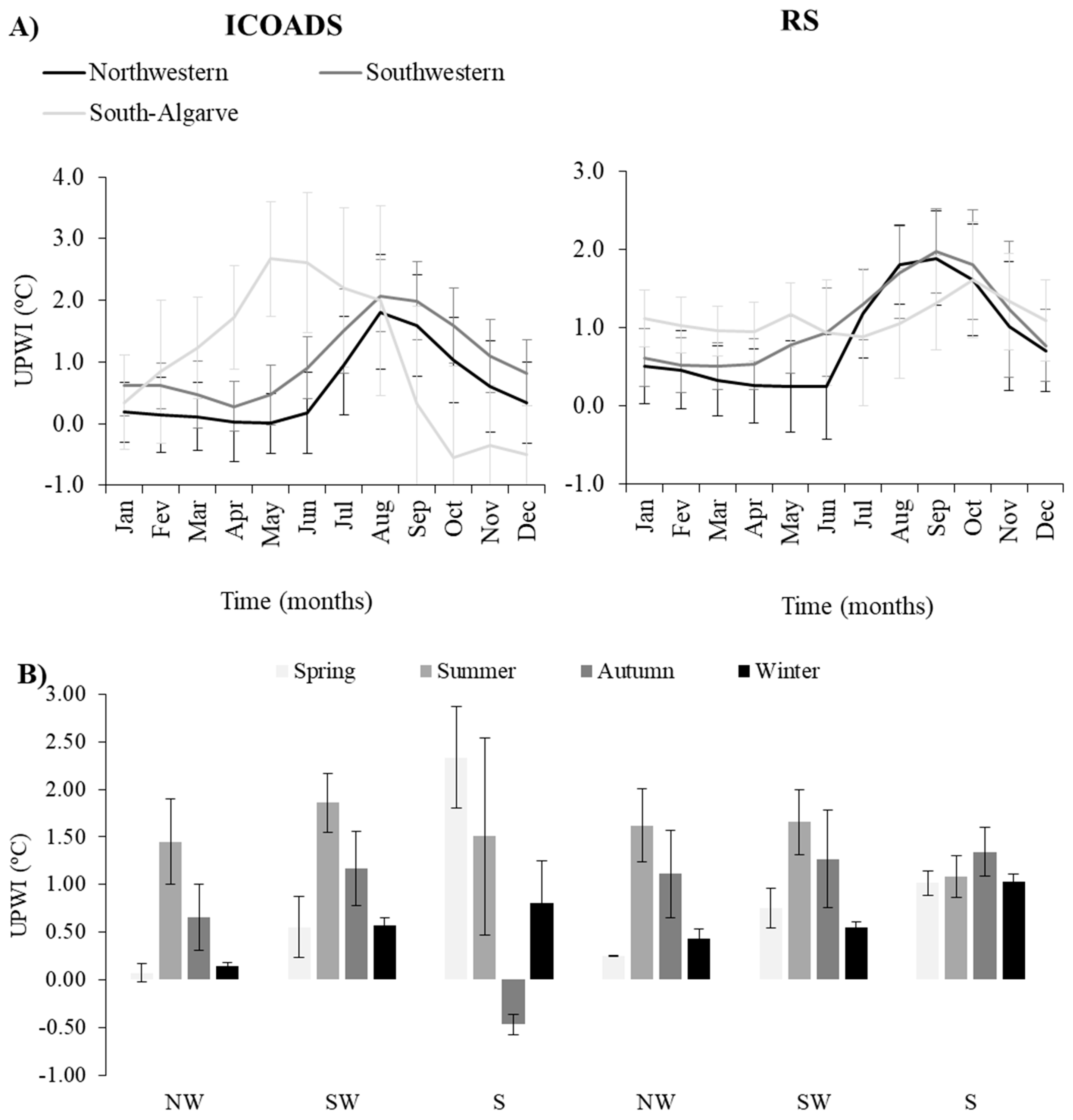
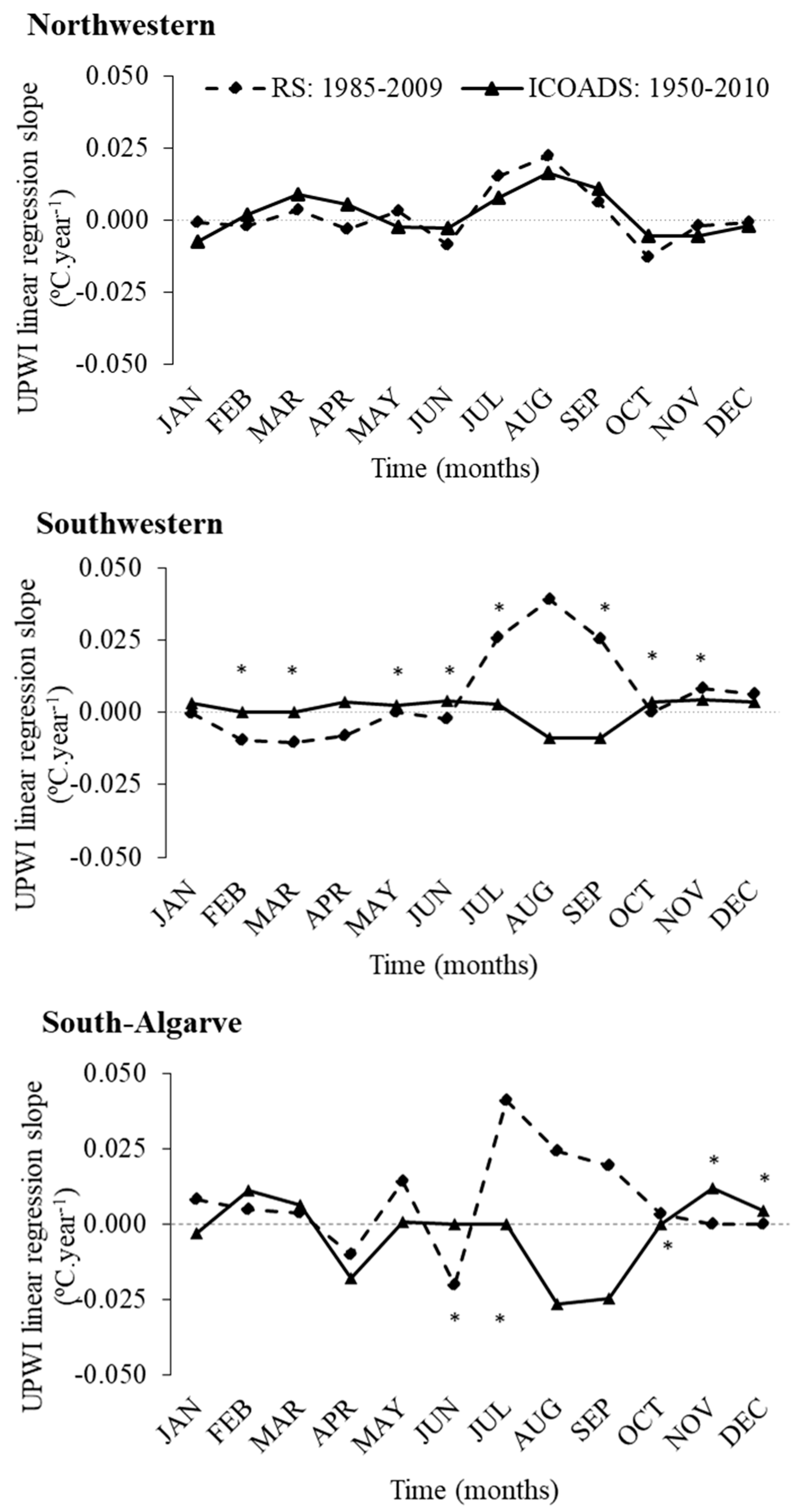
The yearly evolution of monthly UPWI-average (Figure 4; Table 2) show a seasonal pattern (Figure 5) characterized by:

(i)

in the west (NW and SW) coast for both databases (IOCADS and RS) the UPWI index values are lower from January until June peaking in August-September and decreasing after September until December;

(ii)

in S some differences are found among databases regarding the evolution of average monthly UPWI index over the years. In the ICOADS dataset the upwelling season (May to August) differed from NW and SW coasts (July to September).

(iii)

The seasonal pattern of UPWI (Figure 4B) is similar in ICOADS (ICOADS: 1950–2010) and RS (RS: 1985–2009) datasets in NW and SW coasts (increase of UPWI values from spring to summer when it peaks and a decline thereafter in autumn and winter), regardless of the season. In S coast the ICOADS (ICOADS: 1950–2010) seasonal averaged data reveal large UPWI values in spring and summer, with a drop into negative values (downwelling) in autumn. After autumn in S UPWI average seasonal value increased again in winter. In S coast the RS data (RS: 1985–2009) reveal that the UPW seasonal variation in recently decades are similar to seasonal patterns found for both RS (RS: 1985–2009) and ICOADS (ICOADS: 1950–2009) for NW and SW.

(iv)

In NW and S, in recent decades (RS: 1985–2009), an increase in UPWI in Autumn was recorded; in S, in recently decades, a decline of the average Spring and Summer UPW values are observed relative to long-term data (ICOADS: 1950–2002).

Higher yearly UPW intensity rates (slope of the linear regression analyses) were recorded for RS than in ICOADS dataset in June/July-August in SW and S areas (Figure 5; Table 3). In the SW, however, in recent years (RS: 1985–2009) in winter (February and Mars) and early spring (April) of the UPWI index was lower than for long-term data (ICOADS: 1950–2010).

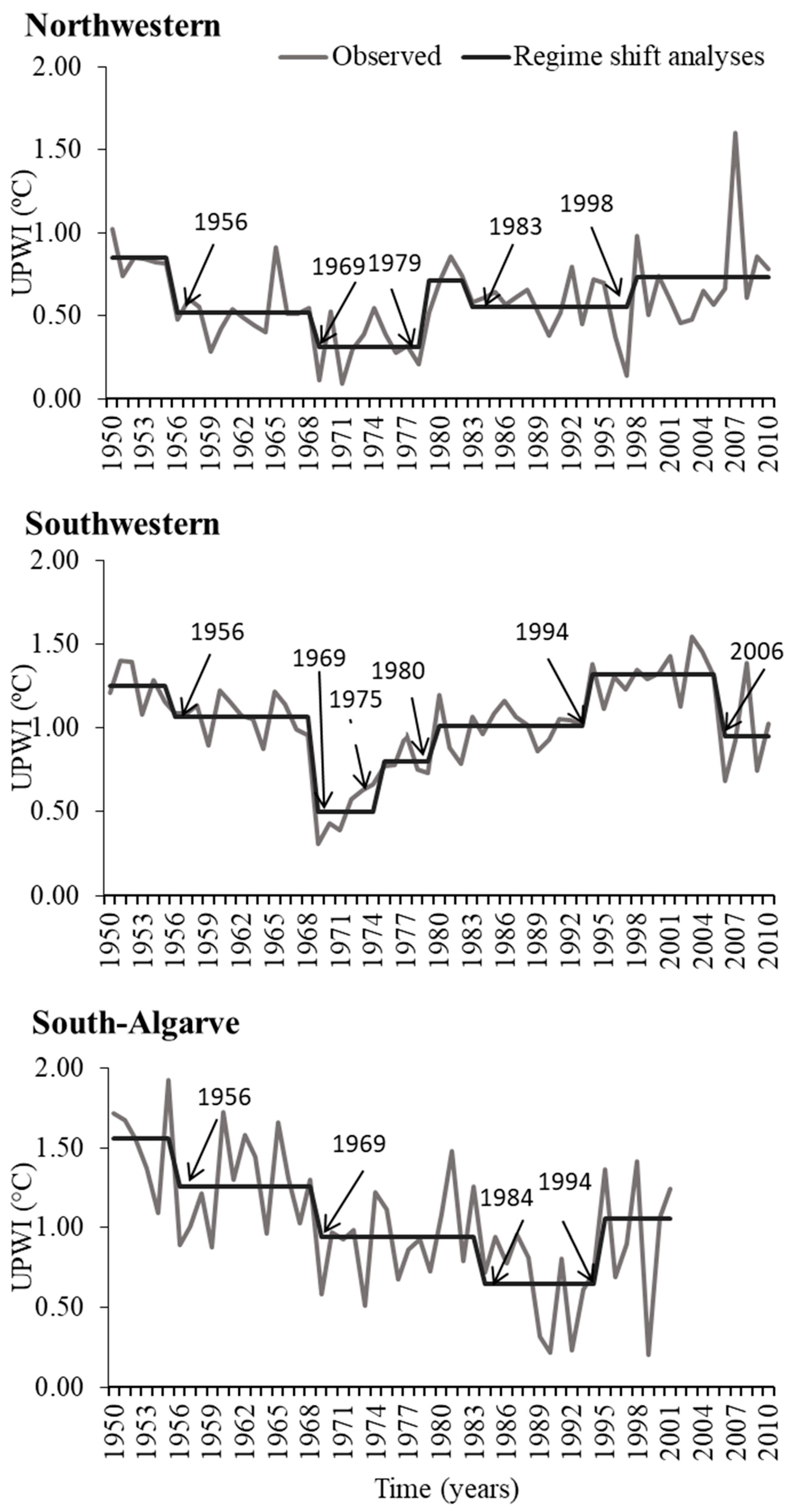
The observed yearly time series trends agree with the estimated Regime Shift Index (RSI) trends (Figure 6;

Table 4. Regime intervals (RSI) separated by shifts detected and confidence level (conf) for each shift detected within every area in the Regime shift analysis (see Figure 6).

Year	Northwest		Southwest		S-Algarve
	RSI	Conf	RSI	Conf	RSI	Conf
1956	−0.846	0.000	−0.876	0.015	−0.604	0.063
1969	−0.077	0.005	−0.900	0.000	−0.681	0.006
1975	0	-	0.902	0.003	0	-
1979	0.822	0.003	0	-	0	-
1980	0	-	0.467	0.003	0	-
1983	−0.195	0.106	0	-	0	-
1984	0	-	0	-	−0.517	0.011
1994	0	-	0.853	0.000	0	-
1995	0	-	0	-	0.887	0.005
1998	0.606	0.074	0	-	0	-
2006	0	-	−1.255	0.039	0	-

). The RSI reveal considerable relaxation from 1956 to 1968 in all areas. Comparing UPWI values using 1950s as the historical period the RSI analyses showed that:

(i)

in NW coast after 1956 a significant drop in UPW intensity was observed over a 23-year period with two markedly sudden changes periods after 1956 and 1969. By 1979 the UPWI rise to values similar to those observed in the beginning of the time series (0.31 °C to 0.71 °C; RSI = 0.82) enduring until 1983 when another shift is detected, with the decrease of the UPW (0.71 °C to 0.55 °C; RSI = −0.20) until 1998 when UPWI rises to similar values of the previous shift (0.55 °C to 0.73 °C; RSI = 0.61); in latter decades UPW intensity is lower than in the early 1950s.

(ii)

in the SW area before 1975, two significant shifts, that lasted 20 years (1956–1968 and 1969–1975), showing a decline in UPWI intensity are found. Afterwards, a clear upwelling intensification was recorded in three consecutive periods that lasted thirteen years: from 1975 to 1980 (0.50 °C to 0.80 °C; RSI = 0.90), from 1980 to 1994 (0.80 °C to 1.01 °C; RSI = 0.45) and from 1994 to 2006 (1.01 °C to 1.32 °C; RSI = 0.85) when the UPWI reached the maximum values in the entire time series and then abruptly drops resulting in a new relaxation period (1.32 °C to 0.95 °C; RSI = −1.26), to values lower than in the early 1950s; in latter decades, the UPWI values are lower than in the early 1950s.

(iii)

in the S area, after mid 1950s (1956), a relaxation of UPWI was recorded in three consecutive periods: 1956–1968, 1969–1983 and 1984–1994 (0.94 °C to 0.65 °C; RSI = −0.52). That means that a significant decline over more than thirteen five years. After 1995, the UPWI values show an intensification period (0.65 °C to 1.06 °C; RSI = 0.89) that continues until the end of the time series (2002); in later decades UPWI intensity is lower than in the early 1950s.

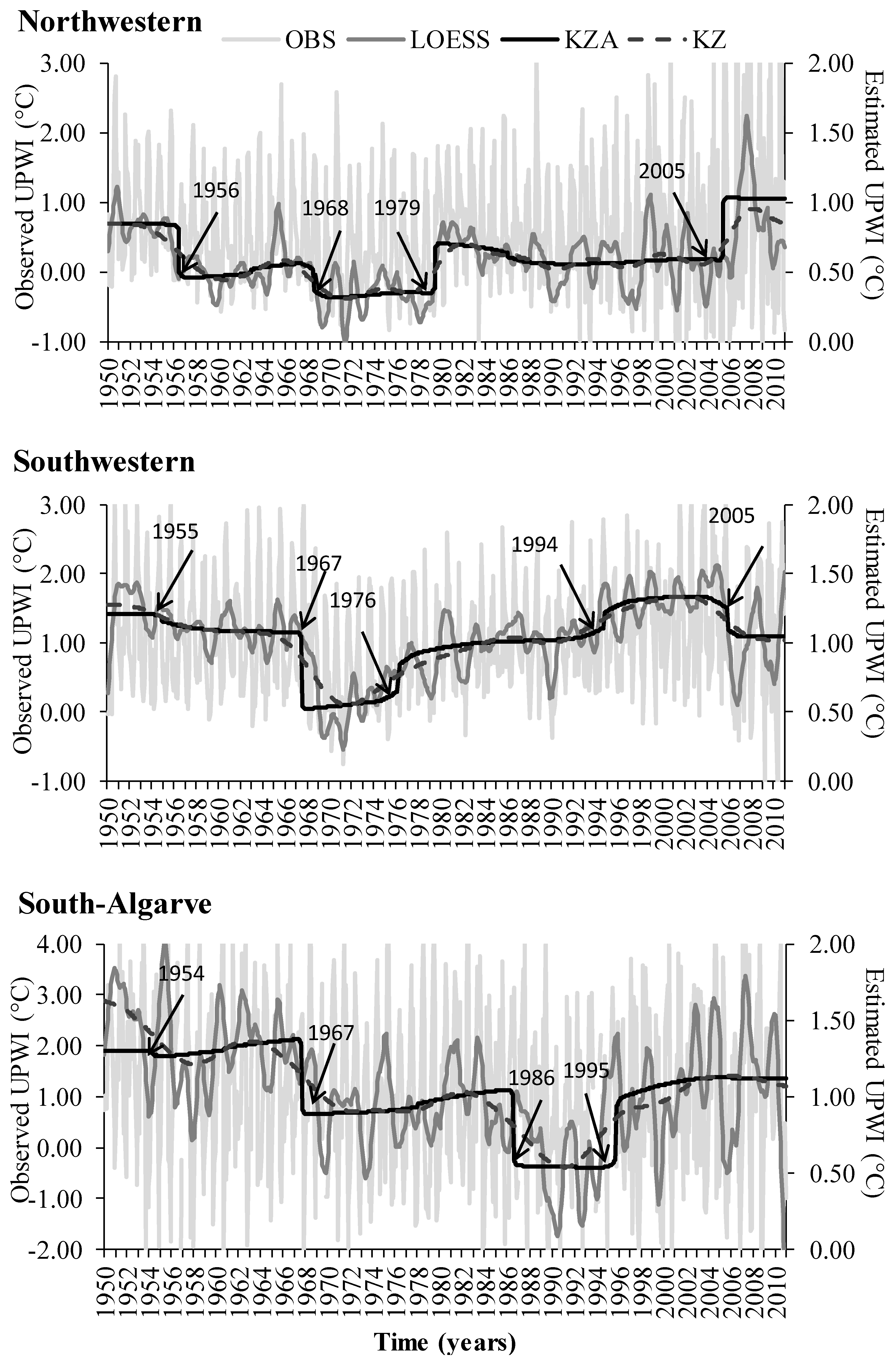
The results from the KZA and KZ analyses (Figure 7;

Table 5. Regime shift periods for each shift detected within the long-term (ICOADS) monthly data in each area with the KZA filter (see Figure 7).

Northwestern				Southwestern			S-Algarve
trend	start	end	trend	start	end	trend	start	end
-	Jan-50	May-56	-	Jan-50	Jun-67	-	Jan-50	Aug-67
decrease	Jun-56	Jul-68	decrease	Jul-67	Feb-76	decrease	Sep-67	Jul-86
decrease	Aug-68	Jun-79	increase	Mar-76	Sep-94	decrease	Aug-86	Sep-95
increase	Jul-79	5-May	increase	Oct-94	5-Oct	increase	Oct-95	10-Dec
increase	5-Jun	10-Dec	decrease	5-Nov	10-Dec

) resemble some periods detected previously by the RSI analyses. In both analyses (RSI and KZA/KZ) the same two UPWI relaxation periods (from 1956 to 1959 and from 1968–1969 to 1979) were observed in the beginning of NW time-series. They lasted over 23 years, with approximately the same time interval recorded for RSI: from 1956 to 1968 and from 1968–1969 to 1979. After 1979 two shifts revealing a progressive increase of UPWI were identified by the KZA and KZ: (i) a first rise of the UPWI from 1979 to 2005 and (ii) afterwards another increase from 2005 onwards, when the UPWI values reach a maximum.

For the SW, KZA and KZ results were equivalent to previous obtained by the RSI analyses.

In S, KZA and KZ overall showed also similar results to those achieved by the RSI analyses, that is a long time period (~35 years) of UPWI decrease with two periods of sudden shifts, rather than 3 as in RSI: from 1967 to 1986 and from 1986 to 1995 (with UPWI reaching a minimum and even negative values, that is downwelling prevalence) followed by recover of the mean UPWI values after 1995.

Comparing the half decade averages of the UPW index long-term time-series from ICOADS dataset (recall Figure 2b) with the results of the sudden changes (Figure 6 and Figure 7), it was possible to observe similar results:

(i)

a decrease of the UPWI half-decadal values until 1970–1975 in NW and 1970-1975s in the SW

(ii)

in S, a continuous decline in half-decadal is observed until 1995.

Overall, RSI, both KZ and KZA and half-decadal observations reveal that in the late 2000s the UPW was lower than in the early 1950–1960s, excluding some peaks in particular observed years/half-decades periods.

4. Discussion

Overall, the long-term and short-term yearly and monthly time-series have the same common trend regardless of the areas, as DFA analyses reveal, although the absolute UPWI values are different. Therefore, this allows comparison among different periods (short term: 1985–2009, and long-term: 1950–2010) as the time series are expected to be similar over time, independently of the data/years availability.

The long-term time-series (ICOADS) enables a good understanding of the evolution of the UPWI across different areas of the Portuguese coast. UPWI time series along the Portuguese Iberian coast is characterized by high inter-annual and monthly variability, as shown by observational data. Considering monthly smoothed-LOESS and linear yearly trends, in the last 60 years (ICOADS: 1950–2010), the results showed that UPWI intensification rate in NW and SW was 0.02 °C decade-1, while in the S UPWI weakened at −0.08 °C decade-1. In S the yearly linear regression trends were statistically significant for both ICOADS and RS data. Moreover, the results also reveal that during the last 25 years (RS: 1985–2010) the entire Portuguese coast experienced a stronger intensification of the upwelling regime with S, presenting the highest increase rate (0.011 °C year-1). Therefore, comparison between recent (RS) and long-term data reveal different information regarding UPWI in two distinct periods.

The sudden shifts analyses (RSI, KZA and KZ) provide complementary information to the observed, linear, and SDL, and reveal episodes of UPWI sudden shifts superimposed to the inter-annual and seasonal variability. The UPWI trend and the shifts interval (increase or decrease the intensity of the UPWI over a period) are coincident among monthly (KZA and KZ) and annual (RSI) sudden change techniques. These analyses showed that in a given shift the change in UPWI values could be several times higher than the inter-annual (yearly linear intensity rate) and seasonal variability. The duration of intervals between successive shifts, regardless of the area, is of several decades (decadal trends). For instance, in S three successive intervals encompassed more than three decades of UPWI weakening. This trend changed in 1994 with a new shift (Figure 6). In the SW coast, a relaxation of UPWI occurred over more than 20 years (1955–1969), and thereafter intensification was recorded for more than three decades. In NW after a relaxation of UPWI, from 1956 until 1969, intensification and relaxation periods alternated over decadal or decadal and half intervals. Different analyses reveal different information that may contribute to a better picture of the UPWI trends and oscillations over the last half-century and results are open to discussion. Analyzing the SST over the Western coast of Iberian Peninsula, [42] observed a cooling period between 1950 and 1974 followed by intense warming between 1974 and 2008, corresponding to our upwelling intensification and relaxation shifts, regardless of the coastal areas. [15] through their work based on measured coastal winds and SST datasets concluded that the upwelling off western Iberia coast had weakened since the 1940s until 2000s. This is in line with the observed results for the three coastal areas until 1967–1968.

Long-term data allow the identification of climatic change periods (the climate normals are 30 years, as defined by the World Meteorological Organization) and such profiles leads to question about large scale cycles (several decades) in UPWI regimes that are still poorly understood. Across Portugal, different coastal areas results showed climatic cycles of UPW relaxation and intensification (more than 30 years) followed by a turnover regime of several decades. This could mean that long-term events or low frequency events are a matter of discussion, but more data would be required to answer such a question.

In NW the yearly UPWI rates (slope of the regression models; Figure 3) were similar among RS and ICOADS and the sudden shifts intervals shorter and more variable than in SW and S, highlighting the more regular UPW behavior at decadal scales (RSI and KZA results) further north. This is consistent with the findings of [22] that showed that warming rates differences between offshore and coast (our UPW index) in NW increase in a similar way. Conversely, in the SW the authors found a larger warming rate offshore than inshore, resulting in an increase contrasting in SST along the years. This also matches our results, as the UPWI increased during that period. Results showed that the upwelling pattern off the SW Iberian Peninsula underwent a slight intensification since 1969. The results from the present work and [22] are corroborated by [43] who showed that between 1989 and 2007 opposite trends in upwelling frequency are found at the western northern limit (NW), where upwelling has been decreasing in recent decades. At the western south edge (SW) there is some evidence of increased upwelling.

In S, different results between present work, [22,43] works are found. According to [22], in S warming of offshore water occur between 1985 and 2008 at a large rate than in nearshore waters. Therefore, the latter authors expected intensification of upwelling between 1985 and 2008. Nevertheless, [43] simulations showed that offshore waters have increased at higher rate in recent decades (1989–2001). The results of [43] are in agreements with S results in the last decades (RS: 1985–2009), as the intensification of UPWI is noted only after 1994. Such an increase in UPWI in recent decades in S (1994–200) is lower than in earlies 1950s and preceded a great period of 30 years of UPWI decline until middle 1990s. In S the RSI and KZA between 1984 and 1994 revealed some of the lowest UPWI values. For S the discrepancy between present results and warming rates in [22] may be attributed to the sparse upwelling events off the south coast and the local particularities of the circulation in the region [44]. Accordingly, [45] stated that the Algarve cannot be assumed to be an upwelling system, defined as a system were upwelling prevails during a substantial part of the year, but rather a region where upwelling events do occur at times.

With our results the hypothesis proposed by [10] and later taken up by [12,17,46,47], which states that the existence of an intensification of coastal upwelling in the last part of the 20th century due to global climate change, is not supported by considering our ICOADS and RS SST short-term data analyses. For instance, such a global pattern was only evident in S (providing linear regression significant slope for RS) and SW (sudden shift analyses). This finding validates the hypothesis taken by [13,15,16] that found evidence of a decrease in coastal upwelling in similar periods in SW. Nonetheless, for the SW and S, a critical remark is observed: (i) since 2005 the upwelling intensity diminished to smaller yet positive UPWI values (prevailing UPW conditions) in SW; and (ii) in S the increased mean values of UPWI are below those recorded in the early 1950s. That is, the UPWI values at the early 1950s in the present study are anchor points for interpretation of recent time series data. Such upwelling intensification described by the above works for the latter 20th century was not observed in NW, where a more stable condition remains, as shown by: (i) weak magnitude regarding consecutive variation in UPWI average shifts values and (ii) shifts among consecutive intensification or relaxation periods in NW contrasting with consecutive shifts with the same trend in SW and S. Therefore, our results show meridional variation of the upwelling behavior with more stable conditions in NW.

Differences in monthly UPWI rates (Figure 4 and Figure 5) between the long-term (ICOADS) and short-term (RS) time series in the SW and S areas during summer months (June/July–August) were observed. It is evident that the strongest upwelling signal takes place between July and September, i.e., corresponding to the peak summer months, as expected for the Iberian Upwelling System [5]. The similarities observed between both datasets in NW could be related to intrinsic features, namely as a transition zone with a particular oceanographic regime [22,48]. The average monthly UPWI results (ICOADS: 1950–2010) reveal that UPW season varied between S (from May to July) and NW and SW (from July to October). ICOADS is a much larger dataset and thus the average values are the results of a large number of years. In S coast the RS data (1985–2009) show that the average mean seasonal variation values in recent decades are similar to seasonal patterns found in both RS and ICOADS for other areas (NW and SW). Therefore, based on RS data, we can postulate about phenological changes in UPWI in S. In fact, in recent decades, individual monthly analyses reveal (slope of the linear regression analyses): (i) relaxation in UPWI in SW in specific winter months (February and Mars) and (ii) intensification of the UPWI in July to September summer months in SW and S coast. [22] found an increase of the SST in SW for the same period. This matches the present results in SW and also in S. Another finding supporting phenological UPWI shifts is the increase of the mean seasonal autumn UPWI values in S from downwelling conditions (ICOADAS: 1950–2010) to strong upwelling values. In recent years the higher mean seasonal UPWI values are found in autumn in S. Moreover, comparing RS and ICOADAS average UPW monthly and seasonal values, results allow us to postulate that the slightly inter-annual increase rate of UPWI in NW and SW, namely in recent decades, are linked to increasing of upwelling intensity in autumn and winter in NW and winter in SW after the mid-1980s.

Upwelling long-term variability studies are controversial, both at a global or regional scale. This applies to [12] results that contrast with other studies after re-analysis of the same data for the same locals with different data sets [49] or many of the studies cited here for the Portuguese Iberian coast and the present work. In part, such differences are also the result of using different time series data analyses (time period), seasonal amalgamation or geographic constraints of the original time series. The question of whether long-term changes in UPWI are associated with inshore, offshore or both SST changes or to other related features (e.g., NAO or currents shifts) is a matter for future studies and analyses.

5. Conclusions

The analysis of SST series (Appendix A) suggests that interannual changes in both offshore and inshore areas were due to similar mechanisms which would be a support for the usage of UPWI as an indicator of upwelling. Since the 1950s, the upwelling in the Portuguese margin has experienced successive weakening periods. Such weakening lasted until the mid/late 1970s in the NW and SW but was prolonged for 20 years more in the S—until 1994. Afterwards, UPWI evolved in different ways:

(i)

in NW more stable conditions were recorded, although the average UPWI values increased in autumn there,

(ii)

in SW an increase in UPWI was recorded after 1970s until 2006 and from July to September,

(iii)

in S a significant increase in inter-annual UPWI intensity rate was observed in latter decades, that also matches an increase of the UPWI rate from July to September; the average UPWI values in Autumn in S denoted a substantial increase from negative (downwelling conditions, ICOADS: 1950–2002) to strong (average values similar to spring and summer) UPWI mean values in latter decades (RS: 1985–2010).

Global results show that:

(i)

sudden, wide amplitude shifts frequently occur, namely in SW and S. These drops of the UPWI usually reach twice the mean UPWI during the previous/following period,

(ii)

These sudden shifts occur at a decadal time-scale,

(iii)

the consecutive intensification or weakening for UPWI shifts (cascading patterns) can last from decades, as in NW where consecutive shifts are more frequent, to more extended periods of more than 30 years, as in SW and S. This large periodicity suggests climatic variability,

(iv)

phenological changes depicted by the increases in UPWI rate are observed in SW and S during the summer of recent decades (RS: 1985–2009).

References

- Pauly, D.; Christensen, V. Primary production required to sustain global fisheries. Nature 1995, 374, 255257. [Google Scholar] [CrossRef]
- Santos, A.M.P.; Chícharo, M.A.; dos Santos, A.; Moita, T.; Oliveira, P.B.; Peliz, A.; Ré, P. Physical–biological interactions in the life history of small pelagic fish in the Western Iberia Upwelling Ecosystem. Prog. Oceanogr. 2007, 74, 192–209. [Google Scholar] [CrossRef]
- Baptista, V.; Leitão, F. Commercial catch rates of the clam Spisula solida reflect local environmental coastal conditions. J. Mar. Syst. 2014, 130, 79–89. [Google Scholar] [CrossRef]
- Leitão, F. Time series analyses reveal environmental and fisheries controls on Atlantic horse mackerel (Trachurus trachurus) catch rates. Cont. Shelf Res. 2015, 111, 342–352. [Google Scholar] [CrossRef]
- Fiúza, A. Upwelling patterns off Portugal. In Coastal Upwelling: Its Sediment Record, Part A; Suess, E., Thiede, J., Eds.; Plenum: New York, NY, USA, 1983. [Google Scholar]
- Relvas, P.; Barton, E.D.; Dubert, J.; Oliveira, P.B.; Peliz, Á.J.; da Silva, J.C.; Santos, A.M.P. Physical oceanography of the Western Iberia Ecosystem: Latest views and challenge. Prog. Oceanogr. 2007, 74, 149–173. [Google Scholar] [CrossRef]
- Wooster, W.; Bakun, A.; McLain, D. The seasonal upwelling cycle along the eastern boundary of the North Atlantic. J. Mar. Res. 1976, 34, 131–141. [Google Scholar]
- Relvas, P.; Barton, E.D. Mesoscale patterns in the Cape Sao Vicente (Iberian peninsula) upwelling region. J. Geophys. Res. Oceans 2002, 107, 28-1–28–23. [Google Scholar] [CrossRef]
- Fiúza, A.; Macedo, M.; Guerreiro, M. Climatological space and time variation of the Portuguese coastal upwelling. Oceanol. Acta 1982, 5, 31–40. [Google Scholar]
- Dickson, R.; Kelly, P.; Colebrook, J.; Wooster, W.; Cushing, D.H. North winds and production in the eastern North Atlantic. J. Plankton Res. 1988, 10, 151–169. [Google Scholar] [CrossRef]
- Moita, M.T.; Vilarinho, M.G.; Palma, A.S. On the Variability of Gymnodium Catenatum Graham Blooms in Portuguese Waters B; Xunta da Galicia and IOC-UNESCO; Reguera, B., Blanco, J., Fernández, M.L., Wyatt, T., Eds.; Harmful Algae: Vigo, Spain, 1998; pp. 118–121. [Google Scholar]
- Bakun, A. Global climate change and intensification of coastal ocean upwelling. Science 1990, 247, 198–201. [Google Scholar] [CrossRef]
- Lavin, A.; Díaz del Rio, G.; Casas, G.; Cabanas, J.M. Afloramiento en el Noroeste de la Península Ibérica. Índices de Afloramiento Para el Punto 43° N, 11° W, Periodo 1990–1999 (Upwelling in the NW of the Iberian Peninsula. Upwelling indexes at 43° N, 11° W, between 1990–1999); Instituto Español de Oceanografia: Madrid, Spain, 2000. [Google Scholar]
- Barton, E.D.; Field, D.B.; Roy, C. Canary current upwelling: More or less? Prog. Oceanogr. 2013, 116, 167–178. [Google Scholar] [CrossRef] [Green Version]
- Lemos, R.T.; Pires, H.O. The upwelling regime off the west Portuguese coast, 1941–2000. Int. J. Climatol. 2004, 24, 511–524. [Google Scholar] [CrossRef]
- Lemos, R.; Sansó, B. Spatio-temporal variability of ocean temperature in the Portugal Current System. J. Geophys. Res. Oceans 2006, 111, C0401. [Google Scholar] [CrossRef]
- Santos, A.M.P.; Kazmin, A.S.; Peliz, A. Decadal changes in the Canary upwelling system as revealed by satellite observations: Their impact on productivity. J. Mar. Res. 2005, 63, 359–379. [Google Scholar] [CrossRef]
- Arístegui, J.; Álvarez-Salgado, X.A.; Barton, E.; Figueiras, F.G.; Hernández-León, S.; Roy, C.; Santos, A.M.P. Oceanography and fisheries of the Canary Current/Iberian region of the eastern North Atlantic. In The Global Coastal Ocean: Interdisciplinary Regional Studies and Syntheses; The Sea, Ideas and Observations on Progress in the Study of the Seas; Robinson, A., Brink, K., Eds.; Harvard University Press: Cambridge, MA, USA, 2006. [Google Scholar]
- Miranda, P.M.A.; Alves, J.M.R.; Serra, N. Climate change and upwelling: Response of Iberian upwelling to atmospheric forcing in a regional climate scenario. Clim. Dyn. 2013, 40, 2813–2824. [Google Scholar] [CrossRef]
- Wang, M.; Overland, J.E.; Bond, N.A. Climate projections for selected large marine ecosystems. J. Mar. Syst. 2010, 79, 258–266. [Google Scholar] [CrossRef]
- Borges, M.F.; Santos, A.M.P.; Crato, N.; Mendes, H.; Mota, B. Sardine regime shifts off Portugal: a time series analysis of catches and wind conditions. Sci. Mar 2003, 67, 235–244. [Google Scholar] [Green Version]
- Relvas, P.; Luís, J.; Santos, A.M.P. Importance of the mesoscale in the decadal changes observed in the northern Canary upwelling system. Geophys. Res. Lett. 2009, 36, L22601. [Google Scholar] [CrossRef]
- Bettencourt, A.; Bricker, S.B.; Ferreira, J.G.; Franco, A.; Marques, J.C.; Melo, J.J.; Nobre, A.; Ramos, L.; Reis, C.S.; Salas, F.; et al. Typology and Reference Conditions for Portuguese Transitional and Coastal Waters Development of Guidelines for the Application of the European Union Water Framework Directive; Sardine Regime Shifts off Portugal: A Time Series Analysis of Catches and Wind Conditions; Instituto da Agua (INAG)—Institute of Marine Science (IMAR): Lisbon, Portugual, 2004; Volume 67, pp. 235–244. [Google Scholar]
- Cunha, M.E. Physical Control of Biological Processes in a Coastal Upwelling System: Comparison of the Effects of Coastal Topography, River Run-off and Physical Oceanography in the Northern and Southern Parts of Western Portuguese Coastal Waters. Ph.D. Thesis, Faculdade de Ciências da Universidade de Lisboa, Lisbon, Portugal, 2001. [Google Scholar]
- Woodruff, S.D.; Worley, S.J.; Lubker, S.J.; Ji, Z.; Freeman, J.E.; Berry, D.I.; Philip Brohan, P.; Kent, E.C.; Reynolds, R.W.; Smith, S.R.; et al. ICOADS Release 2.5: Extensions and enhancements to the surface marine meteorological archive. Int. J. Climatol. 2011, 31, 951–967. [Google Scholar] [CrossRef]
- Kilpatrick, K.A.; Podesta, G.P.; Evans, R. Overview of the NOAA/NASA advanced very high resolution radiometer Pathfinder algorithm for sea surface temperature and associated matchup database. J. Geophys. Res. Oceans 2001, 106, 9179–9197. [Google Scholar] [CrossRef]
- Santos, A.M.P.; Borger, M.F.; Groom, S. Sardine and horse mackerel recruitment and upwelling off Portugal. ICES J. Mar. Sci. 2001, 58, 589–596. [Google Scholar] [CrossRef]
- Jacox, M.G.; Edwards, C.A.; Hazen, E.L.; Bograd, S.J. Coastal upwelling revisited: Ekman, Bakun, and improved upwelling indices for the U.S. West Coast. J. Geophys. Res. Oceans 2018, 123, 7332–7350. [Google Scholar] [CrossRef]
- Nykjaer, L.; Van Camp, L. Seasonal and interyearly variability of coastal upwelling along northwestern Africa and Portugal from 1981 to 1991. J. Geophys. Res. 1994, 99, 14197–14208. [Google Scholar] [CrossRef]
- Narayan, N.; Paul, A.; Mulitza, S.; Shulz, M. Trends in coastal upwelling intensity during the late 20th century. Ocean Sci. 2010, 6, 815–823. [Google Scholar] [CrossRef] [Green Version]
- Zuur, A.F.; Ieno, E.N.; Smith, G.M. Analysing Ecological Data; Springer: New York, NY, USA, 2007. [Google Scholar]
- Zuur, A.F.; Fryer, R.J.; Jolliffe, I.T.; Dekker, R.; Beukema, J.J. Estimating common trends in multivariate time series using dynamic factor analysis. Environmetrics 2003, 15, 665–685. [Google Scholar] [CrossRef]
- Zuur, A.F.; Pierce, G.J. Common trends in Northeast Atlantic squid time series. J. Sea Res. 2004, 52, 57–72. [Google Scholar] [CrossRef]
- Zuur, A.F.; Tuck, I.D.; Bailey, N. Dynamic factor analysis to estimate common trends in fisheries time series. Can. J. Fish. Aquac. Sci. 2003, 60, 542–552. [Google Scholar] [CrossRef]
- Rodionov, S.N. A brief overview of the regime shift detection methods. In Large-Scale Disturbances (Regime Shifts) and Recovery in Aquatic Ecosystems: Challenges for Management Toward Sustainability; Velikova, V., Chipev, V., Eds.; UNESCO-ROSTE/BAS Workshop on Regime Shifts: Varna, Bulgaria, 2005. [Google Scholar]
- Rodionov, S.N. A sequential algorithm for testing climate regime shifts. Geophys. Res. Lett. 2004, 31, L09204. [Google Scholar] [CrossRef]
- Rodionov, S.N. Detecting regime shifts in the mean and variance: Methods and specific examples. In Large-Scale Disturbances (Regime Shifts) and Recovery in Aquatic Ecosystems: Challenges for Management toward Sustainability; Velikova, V., Chipev, N., Eds.; UNESCO-ROSTE/BAS Workshop on Regime Shifts: Varna, Bulgaria, 2005. [Google Scholar]
- Yang, W.; Zurbenko, I. Kolmogorov–Zurbenko filters. WIREs Comput. Stat. 2010, 2, 340–351. [Google Scholar] [CrossRef]
- Yang, W.; Zurbenko, I. Kzft: Kolmogorov–Zurbenko Fourier transform and application. 2006; Unpublished work. [Google Scholar]
- Close, B.; Zurbenko, I. Kza: Kolmogorov–Zurbenko adaptive algorithm for the image detection. 2013; Unpublished work. [Google Scholar]
- Zurbenko, I.G.; Porter, P.S.; Rao, S.T.; Ku, J.Y.; Gui, R.; Eskridge, R.E. Detecting discontinuities in time series of upper air data: Development and demonstration of an adaptive filter technique. J. Clim. 1996, 9, 3548–3560. [Google Scholar] [CrossRef]
- Santos, F.; Gomez-Gesteira, M.; deCastro, M. Coastal and oceanic SST variability along the western Iberian Peninsula. Cont. Shelf Res. 2011, 31, 2012–2017. [Google Scholar] [CrossRef]
- Alves, J.M.R.; Miranda, P.M.A. Variability of Iberian upwelling implied by ERA-40 and ERA-Interim reanalyses. Dyn. Meteorol. Oceangr. 2013, 65, 19245. [Google Scholar] [CrossRef]
- Lafuente, J.G.; Ruiz, J. The Gulf of Cádiz pelagic ecosystem: A review. Prog. Oceanogr. 2007, 74, 228–251. [Google Scholar] [CrossRef]
- Garel, E.; Laiz, I.; Drago, T.; Relvas, P. Characterisation of coastal counter-currents on the inner shelf of the Gulf of Cadiz. J. Mar. Syst. 2016, 155, 19–34. [Google Scholar] [CrossRef] [Green Version]
- McGregor, H.; Dima, M.; Fischer, H.; Mulitza, S. Rapid 20thcentury increase in coastal upwelling off northwestern Africa. Science 2007, 315, 637–639. [Google Scholar] [CrossRef] [PubMed]
- Cropper, T.E.; Hanna, E.; Bigg, G.R. Spatial and temporal seasonal trends in coastal upwelling off Northwestern Africa, 1981–2012. Deep Sea Res. Part I Oceanogr. Res. Pap. 2014, 86, 94–111. [Google Scholar] [CrossRef]
- Gómez-Gesteira, M.; Gimeno, L.; deCastro, M.; Lorenzo, M.N.; Alvarez, I.; Nieto, R.; Taboada, J.J.; Crespo, A.J.C.; Ramos, A.M.; Iglesias, I.; et al. The state of climate in NW Iberia. Clim. Res. 2011, 48, 109–144. [Google Scholar] [CrossRef] [Green Version]
- Varela, R.; Álvarez, I.; Santos, F.; deCastro, M.; Gómez-Gesteira, M. Has upwelling strengthened along worldwide coasts over 1982-2010? Sci. Rep. 2015, 5, 10016. [Google Scholar] [CrossRef]
- Sen, P.K. Estimates of the regression coefficient based on Kendall’s tau. J. Am. Stat. Assoc. 1968, 63, 1379–1389. [Google Scholar] [CrossRef]
- Theil, H. A Rank-Invariant Method of Linear and Polynomial Regression Analysis. In Henri Theil’s Contributions to Economics and Econometrics. Advanced Studies in Theoretical and Applied Econometrics, vol 23; Raj, B., Koerts, J., Eds.; Springer: Dordrecht, The Netherlands, 1992. [Google Scholar] [CrossRef]
- Thorsten, P. Trend: Non-Parametric Trend Tests and Change-Point Detection. R package version 1.1.1. 2018. Available online: https://CRAN.R-project.org/package=trend (accessed on 22 January 2018).
Figure 1.
Map of the Portuguese coast, showing the studied areas (Northwestern—NW, Southwestern—SW, and South-Algarve—S) and information on the International Comprehensive Ocean—Atmosphere Data Set (ICOADS) point data (a) and satellite (b) observation points/pixels used to extract the mean sea surface temperature in coastal (till 200 m isobath) and offshore areas.
Figure 2.
(A) ICOADS (1950-2010 for NW and SW and 1950-2001 for S) and RS (1985-2009) monthly upwelling Index (UPWI) means for Portuguese coastal areas; (B) Long-term half-decadal (ICOADS) UPWI mean values and corresponding standard deviations intervals time series in study areas.
Figure 3.
Observed and linear adjusted annual ICOADS (1950-2010 for NW and SW and 1950-2001 for S) and upwelling Index (UPWI) time series by study areas: Northwestern (NW), Southwestern (SW) and South-Algarve (S).
Figure 4.
(A) Average monthly upwelling Index (UPWI) and (B) average seasonal UPWI for the ICOADS (1950–2010 for NW and SW and 1950–2001 for S) and RS (1985–2009) observed data by study areas. Northwestern (NW), Southwestern (SW) and South-Algarve (S).
Figure 5.
Yearly upwelling Index (UPWI) rates, based on the linear regression models, for the ICOADS (1950–2010 for NW and SW and 1950–2001 for S) and RS (1985–2009) observed data by study areas: Northwestern (NW), Southwestern (SW) and South-Algarve (S). *-statistical significant regressions (p < 0.1) for either ICOADS and RS (see Table 3).
Figure 6.
Sudden shifts in the Upwelling Index (UPWI) by study area for ICOADS data (1950–2010 for NW and SW and 1950–2001 for S). The black lines representing the RSI—Regime Shift Index. The inflexion years in sudden shifts analyses are indicated with arrows (see also Table 4).
Figure 7.
Monthly observed, Kolmogorov-Zurbenko (KZ) and Kolmogorov-Zurbenko Adaptative (KZA) filters trends for upwelling Index (UPWI) by study area: Northwestern (NW), Southwestern (SW) and South-Algarve (S).