Can the Quality of the Potential Flood Risk Maps be Evaluated? A Case Study of the Social Risks of Floods in Central Spain


1
Department of Geodynamics, Stratigraphy and Paleontology, Complutense University of Madrid, E-28040 Madrid, Spain
2
Ferrovial Agroman, US Corp., North America Headquarters, Austin, TX 78759, USA
3
Geological Survey of Spain (IGME), Ríos Rosas 23, E-28003 Madrid, Spain
*
Author to whom correspondence should be addressed.
Water 2019, 11(6), 1284; https://doi.org/10.3390/w11061284
Submission received: 9 May 2019
/
Revised: 17 June 2019
/
Accepted: 18 June 2019
/
Published: 20 June 2019
(This article belongs to the Special Issue Flood Risk Assessments: Applications and Uncertainties)
Abstract
:Calibration and validation of flood risk maps at a national or a supra-national level remains a problematic aspect due to the limited information available to carry out these tasks. However, this validation is essential to define the representativeness of the results and for end users to gain confidence in them. In recent years, the use of information derived from social networks is becoming generalized in the field of natural risks as a means of validating results. However, the use of data from social networks also has its drawbacks, such as the biases associated with age and gender and their spatial distribution. The use of information associated with phone calls to Emergency Services (112) can resolve these deficiencies, although other problems are still latent. For example, a bias does exist in the relationship between the size of the population and the number of calls to the Emergency Services. This last aspect determines that global regression models have not been effective in simulating the behavior of related variables (calls to Emergency Services–Potential Flood Risk). Faced with this situation, the use of local regression models (such as locally estimated scatterplot smoothing (LOESS)) showed satisfactory results in the calibration of potential flood risk levels in the Autonomous Community of Castilla-La Mancha (Spain). This provides a new methodological path to the calibration studies of flood risk cartographies at national and supra-national levels. The results obtained through LOESS local regression models allowed us to establish the correct relationship between categorized potential risk levels and the inferred potential risk. They also permitted us to define the cases in which said levels differed ostensibly and where potential risk due to floods assigned to those municipalities led to a lower level of confidence. Therefore, based on the number of calls to the Emergency Service, we can categorize those municipalities that should be the subject of a more detailed study and those whose classification should be revised in future updates.
1. Introduction and Objectives: The Assessment of Quality of Maps and the Peculiarities of Flood Risk Maps
Floods are probably the natural process with the greatest temporal and spatial recurrence affecting society throughout the world. Data compiled by “The international disasters database” for the period 1900–2018 [1], for example, show that maximum annual flooding was reached during the year 2008. That is why flood risk management has become an essential tool from both social and economic perspectives to reduce both economic losses and loss of human lives. However, the extension of the territory conditions the flood risk analysis approach [2]; each scale of work requires the use of different methods of analysis, and the results must satisfy different uses. Depending on the spatial extent of the analysis, de Moel et al. [2] propose four scales (supra-national, macro-scale or national, meso-scale or regional, and micro-scale or local). This does not mean they are isolated, because some of the analysis methodologies are valid for different scales (in many cases by using grouping techniques or by simplifying calculation processes). Approaches, analysis techniques, results, uncertainties, and processes used for validation of the results associated with each of these four working scales are included in de Moel et al. [2]. The processes used to validate results are key points that will require a greater effort in the future (regardless of the scale of work of the analysis), since they also determine the utility for end users [3]. Thus, de Moel et al. [2] raise the need to focus efforts on obtaining post-disaster information (with as much detail as possible) as a fundamental tool to improve the calibration, the validation, and the representativeness of flood risk models.
When the study area is large (macro-scale analysis and above), one of the main problems we face in validation and calibration of the results is the lack of post-event information uniformly distributed throughout the territory. This lack of validation, as has been shown in several previous works [4,5,6], can lead to an over-estimation of risk from a quantitative analysis point of view. However, other authors showed that this quantitative overestimation did not have a negative influence in terms of prioritization between localities for future, more detailed work [6,7]. The quantitative magnitude of the risk varies but not its scalar ordering and ranking. This problem of validation and calibration of the results was also considered by Dottori et al. [8]; they state that the validation of supra-national models of flood hazard is limited by the scarce availability of reference maps of flooded areas. This is largely the case in Africa, Asia, and South America, and in developing countries in general [9].
In cases of both macro-scale (national) and supra-national scale models, validation of the results is affected by the scarce availability of contrast information—an aspect favored by the spatial and the temporal discontinuity in the occurrence of floods. The particularities of flood risk maps contribute to this situation [10] in which the use of information referring to flooded areas in river floodplains (through, for example, the use of aerial or satellite images) does not necessarily produce good results in locations of great interest for flood risk analysis; for example, the purpose of validation of flood risk models based on data from insurance policies [11]. Although the extension of the affected areas remains homogeneous (with respect to the validation through data from flooded areas), a tendency to reduce the damage associated with the flood events considered is observed.
Another form of risk map calibration used mainly in the analysis of flood hazards (by hydro-dynamics modeling) is one that was proposed at the beginning of 2010s. It suggested using data contributed through citizen collaboration [12,13,14,15,16]. It is worth highlighting the state of the art of these citizen observation techniques [17] carried out by Assumpção et al. [18], which includes not only data provided by direct observation but also those provided by social networks. The use of data from social networks has gained importance in recent years, with a proliferation of works in which these data are used for flood modeling and monitoring [19,20,21,22,23,24], the spatial planning of settlements for displacement by floods [25], as well as other natural disasters [26]. However, the use of data from citizen collaboration (in its different modalities) is not trivial despite the great interest in using such sources in the assessment of natural hazards [27]. As pointed out by Rosser et al. [28], the data have generally not undergone any type of validation or quality assessment [29] and may contain deliberate or unintentional biases [30].
In addition, as noted by Xiao et al. [30], socio-economic factors play a major role (of greater importance than the size of populations or the magnitude of associated natural disasters) in the “natural disasters–social networks” relationship. This means that factors such as age, sex, educational and economic level, or location in urban or rural areas can condition this relationship, since they also condition the access and the use of social networks. This combination of factors and their relationship with the use of social networks can be a negative handicap for the calibration of risk analysis in rural areas (with an ageing population and, in general, lower educational and economic levels).
This study tries to overcome some of the limitations previously raised. First, a flood risk analysis model was developed in the region of Castilla-La Mancha (located in the center of the Iberian Peninsula), which mainly focused on the social analysis of flood risk. Although the analysis could be administratively placed on a regional scale, the autonomous community of Castilla-La Mancha covers a very large area (greater than over 50% of the countries in Europe), meaning that the study could be placed within the macro or the national scale. The flood risk analysis (RICAM project) was developed for the Civil Protection Service (regional government of Castilla-La Mancha), thus the validation of the results obtained was of vital importance. To this end, a validation/calibration model of potential flood risk analysis was proposed (associated with different flood return periods or recurrence probabilities), and this analysis was based on the information gathered in the emergency telephone (112) of the Castilla-La Mancha region. This approach was based on the hypothesis of a higher accessibility to this service (emergency telephone) than to other social networks and a less biased calibration due to the socio-economic factors of the population.
Therefore, two main objectives were achieved. The first objective was to propose a methodological approach for the analysis of potential flood risks (with a predominantly social focus) with the objective of obtaining a flood risk level ranking (using a multi-criterion analysis-geographic information system approach, MCA-GIS). The second objective was to propose a validation method for the results obtained in the previous phase (with the combination of Emergency Service 112–locally estimated scatterplot smoothing (LOESS)). The ultimate goal was to prioritize mitigation actions and maximize the efficiency of economic investments.
2. Study Site
2.1. Environmental Description
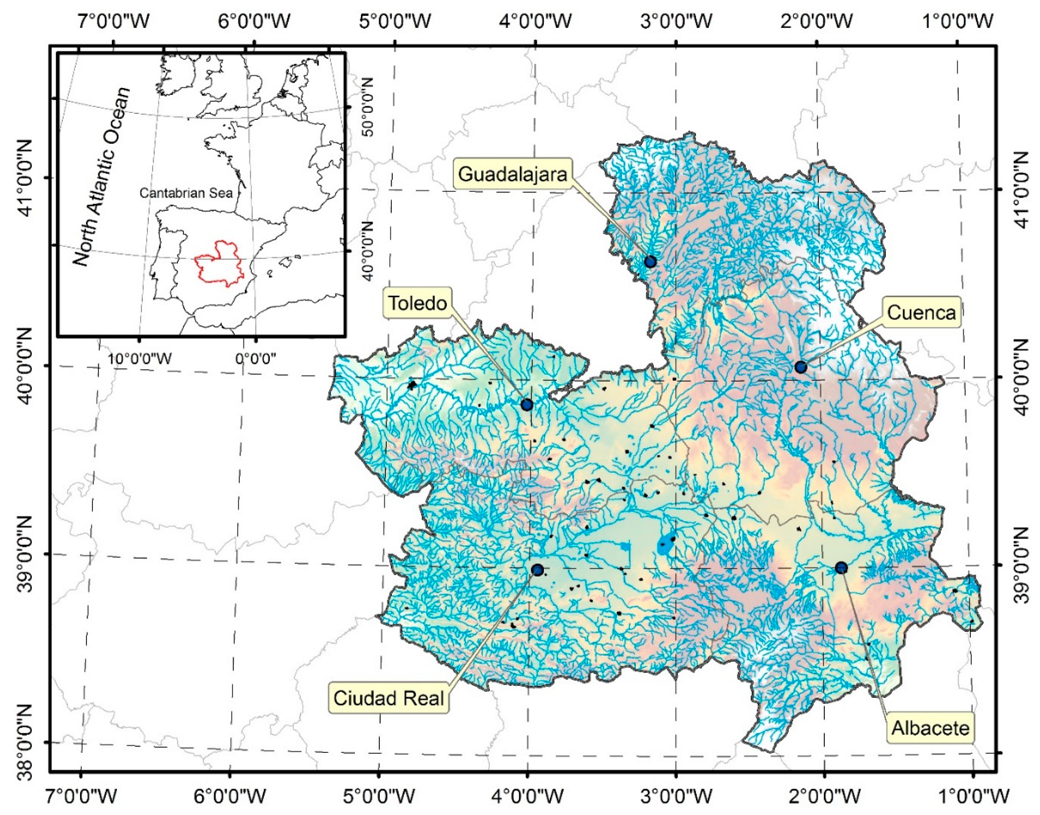
The region of Castilla-La Mancha (Figure 1) is located in the southern half of the Iberian Peninsula (between latitudes 38°01’ and 41°20’ N and longitudes 0°55’ to 5°24’ W), occupying the greater part of the South Sub-plateau with an area of 79,226 km2.
The region has an average altitude between 600 and 700 m above sea level (a.s.l.). The maximum and the minimum elevations can be found in the Pico Lobo (2262 m) and in the floodplain of the Tagus River (289 m) at the western boundary of the province of Toledo. The autonomous community of Castilla-La Mancha has three major relief groups. The first of them corresponds to a plain that covers the entire central area of the autonomous community, and it is thus called “La Mancha plain”. The relief of this area fluctuates between 500–1000 m high, and it makes up close to 70% of the total territory.
The second group is associated with the most important reliefs, which are mainly located in the northeastern boundary of the region (where there are mountains peaks above 2000 m a.s.l.). The foothills of other major reliefs of the Iberian Peninsula (Cordillera Bética, Cordillera Ibérica, Sierra Morena, and Central System) are in the region of Castilla-La Mancha where altitudes can range between 1000 and 1500 m a.s.l. Finally, the third orographic group includes the valleys of the main rivers that drain the territory of the autonomous community. The largest area of this group is associated with flood plains and adjacent areas of the Tagus and the Guadiana Rivers and their main tributaries.
Castilla-La Mancha has a Mediterranean climate, although the special latitudinal and geographical configuration of the region makes it very continentalized [31]. The weather is characterized by the seasonality of its temperatures, a clear period of summer drought (usually very severe in both duration and intensity), and the irregularity of annual rainfall. The distribution of precipitation is conditioned by the sequence of anticyclonic or cyclonic conditions throughout the year. The weather is anticyclonic in summer and winter (warm and cold anticyclonic) and cyclonic in autumn and spring equinoxes. In terms of annual rainfall [32], the total volume is 41,000 hm3, which is equivalent to an average of 510 mm m−2 year−1, with maximum values associated with the Tagus and the Guadalquivir river basins (590 mm m−2 year−1) and a minimum value for the Segura river basin (410 mm m−2 year−1). Rainy days can vary between 53 and 78 days, with very few days of snow except in the northeast quadrant, which clearly stands out from the rest (19 days). Storms, however, affect the entire territory in a similar way (between 15 and 25 days a year).
The waters of the autonomous community of Castilla-La Mancha are distributed among eight hydrographic basins of the Iberian Peninsula. The most important are the Tagus, the Guadiana, and the Júcar basins, while the area covered by the remaining five can be considered marginal. In general, the main rivers and their tributaries have the usual characteristics of Mediterranean rivers with a very low water level in summer, a maximum in spring, a secondary maximum in autumn, and a secondary minimum in winter. Only the rivers with their headwaters in the central system have a nivo-pluvial supply; most are supplied with rainwater, often through large avenues. This pattern translates into an annual distribution of floods that is concentrated from September to April.
2.2. Social Description
The autonomous community of Castilla-La Mancha is administratively divided into five provinces in which approximately 1.8 million inhabitants live (with an average population density of 22.25 inhabitants per km2). These five provinces are subdivided into 919 municipalities with 1487 population centers. The largest population center of the autonomous community corresponds to the city of Albacete (capital of the homonymous province) with 149,000 inhabitants. Next are other provincial capitals (Ciudad Real, Cuenca, Guadalajara, and Toledo, also with names homonymous to those of their provinces) and the city of Talavera de la Reina (the second largest population in the autonomous community). All of them have populations that fluctuate between 50,000 and 75,000 inhabitants. In only 54 of the remaining 913 municipalities does the number of inhabitants exceed 5000. These data show that the population is spread out over a large number of small population centers. Thus, the average population values per municipality stands at around 2000 inhabitants, while the average inhabitants per population centers would be reduced to 1200.
Population distribution by age and gender is very similar in all the provinces, and the population pyramid reaches a maximum (independent of sex) between the ages of 40 and 60 with a second peak in the age range of 80 and 90. While the male population is slightly higher in the young and the middle-aged groups, the trend is reversed for the older population in which female inhabitants dominate.
This trend in population distribution has been preferentially observed in the most populated municipalities. However, smaller municipalities (those with a total population of less than 2000 inhabitants) do not fit very well into the age distribution pattern noted above. In these small urban centers, population distribution remains stable throughout all of the age ranges used (five year intervals), and the maxima, which is poorly defined, moves upward, which points us towards aging populations. This situation is important and should be taken into account in a flood risk analysis with a social approach, as older population groups may be more vulnerable. To conclude, the population scenario of the autonomous community of Castilla-La Mancha indicates that 635 of its 919 municipalities have a population of less than 1000 inhabitants (representing 69% of municipalities) in which aging is more evident.
Finally, from a socio-economic point of view, services are considered the main productive sector of the autonomous community, accounting for almost 60% of its gross domestic product (GDP). This sector is followed by industry (23% of GDP), whose major activities include energy production, agro-food industry, wood and furniture manufacturing, leather and footwear, production of non-metallic minerals, and oil refining. Finally, the influence that the agricultural sector has on the autonomous community (7.5% of GDP), where rain-fed cereals, vines, and olive trees are the main crops, cannot be ignored.
3. Data Sources and Methodologies
3.1. The Flood Risk Maps of the PRICAM Project (MCA and GIS)
The RICAM project [33] was developed between 2005 and 2007 to comply with the Spanish civil protection legislation in terms of risk prevention against floods in the national territory [34]. Specifically, the project formed the basis of knowledge for the development of the Special Plan of Civil Protection against the Flood Hazard of the autonomous community of Castilla-La Mancha (PRICAM, level II plan, regional scope) for which the autonomous community itself is responsible.
The objective of the PRICAM project was to determine the social risk of floods and the categorization of the different population centers of Castilla-La Mancha. These administrative entities were therefore established as units of analysis in the project. PRICAM was initially a flood risk study that shared characteristics associated with macro- and meso-scale studies [2] on the 79,000 km2 extension of the autonomous community of Castilla-La Mancha. The PRICAM project considered floods that were produced from the typologies listed below:
- River flooding,
- In situ rainfall flooding,
- Dam failure flooding.
For flood risk analysis, MCA techniques supported in a GIS environment were used. As stated by Meyer et al. [35], the use of spatial MCA techniques began to spread in different fields of study from the last quarter of the 20th century and the first years of the 21st century, including the analysis of flood risk [35,36,37,38]. This analysis approach could be classified into the parametric approaches to the study of flood risks [39,40,41]. One of the main factors in the spatial MCA analysis is the allocation of weights for the different variables used. In this case, a simplified variant of the so-called Delphi method consensus was applied [42,43]. Simplification consisted of eliminating the second circulation of the results of the first round of surveys, considering it inoperative with adequate convergence of answers in the first round. The importance assigned by the experts to each of the variables was therefore considered in the MCA model (Table 1), reducing the subjectivity of the analysis and the results obtained [44].
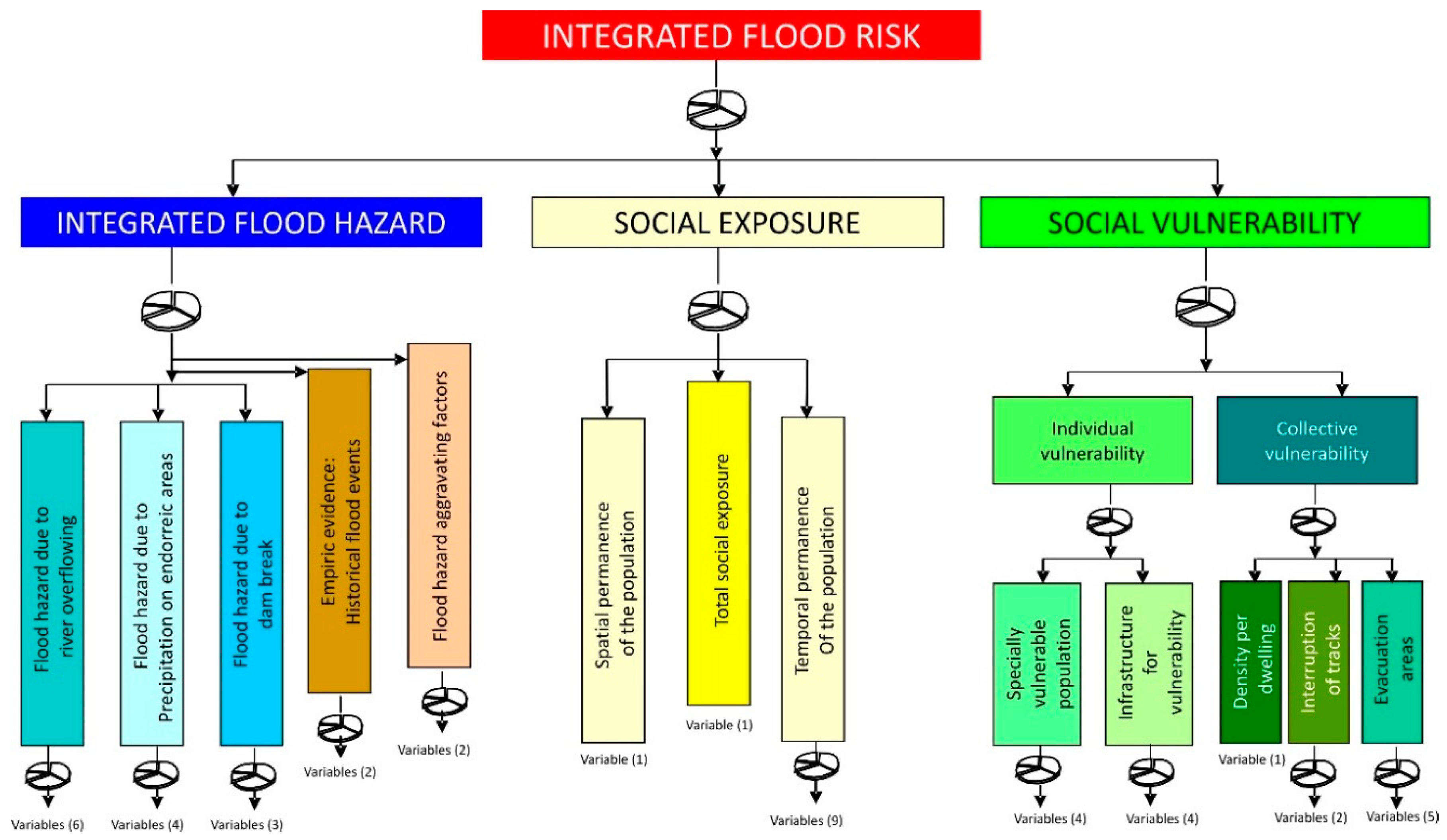
Within the spatial MCA, up to 44 variables were evaluated (17 associated with flood hazard, 11 with flood exposure, and 16 with flood vulnerability), as can be seen in Figure 2. The sources of information and data for the estimation of the different variables considered within the MCA were mostly official. This information was in both vector and raster format. The topography came from raster datasets with a spatial resolution of 100 × 100 m. Meteorological variables were contained from raster datasets with a resolution of 500 × 500 m [45]. Furthermore, geology, lithology, and geomorphology data came from two cartographies at a scale of 1:200 k and 1:400 k, both in vector format [46]. All socio-economic information had its origin in the Ministry of Public Administration of the Spanish Government. All datasets were supported by a GeoDatabase in ArcGIS (ESRI Geosystems).
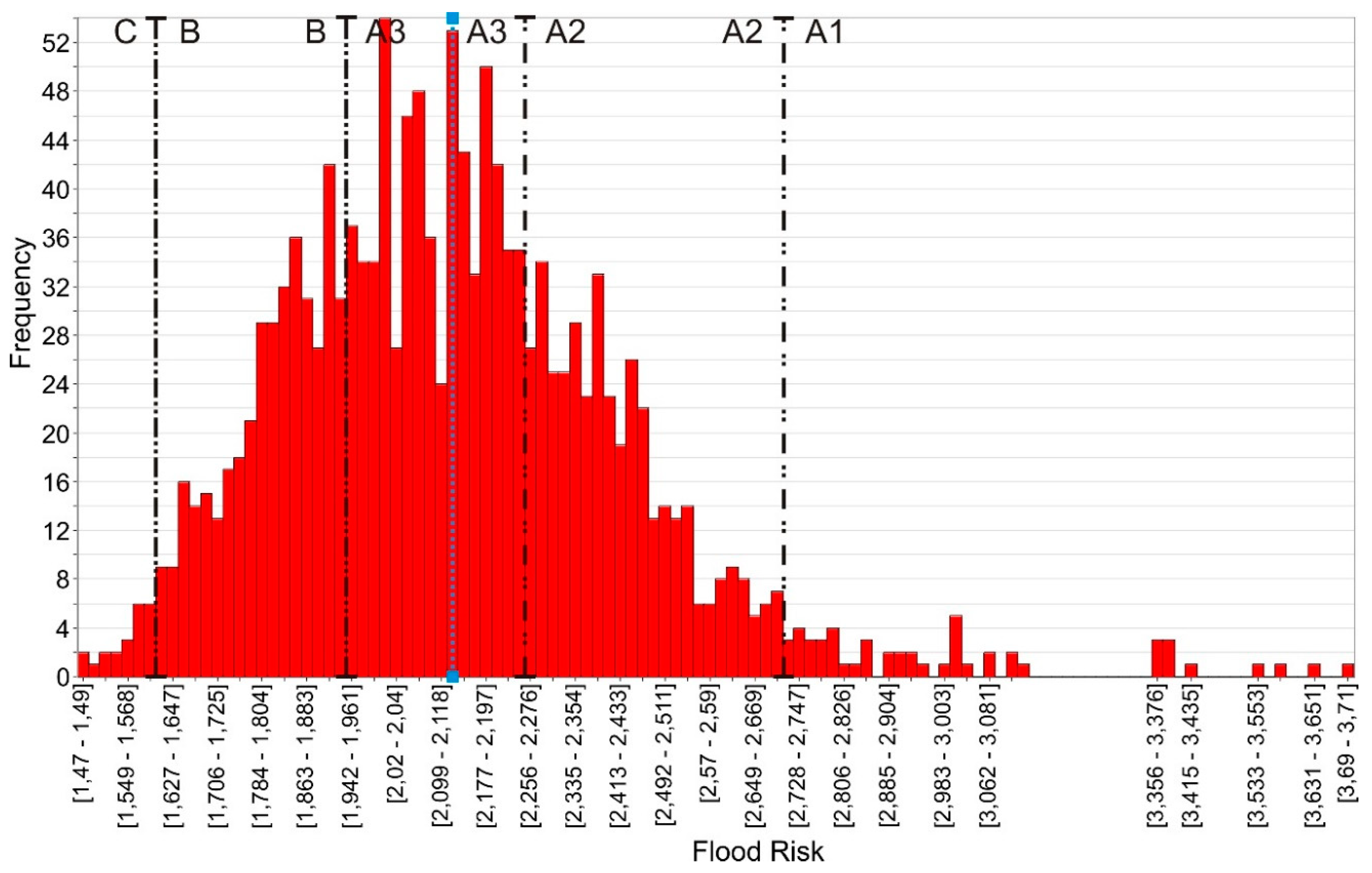
Results for each criterion (variable), factor, and total integrated risk were obtained from the MCA and the whole of Castilla-La Mancha. The scales were quantitative and qualitative (normally with values between one and five) or three classes (low, medium, and high). In the case of the integrated total risk map, the scale of the Basic Directive for Civil Protection against Flood Hazards [34] was used, which established classes A1, A2, A3, B, and C (Table 2). The spatial units for estimating the flood risk were the 1487 population centers of Castilla-La Mancha, to which we added the protected natural areas and the campsites. Categorization of population centers into risk classes based on the statistical analysis of flood risk values (flood frequency histogram) and binary graphs (risk vs. hazard) resulted in the interval classes reflected in Figure 3.
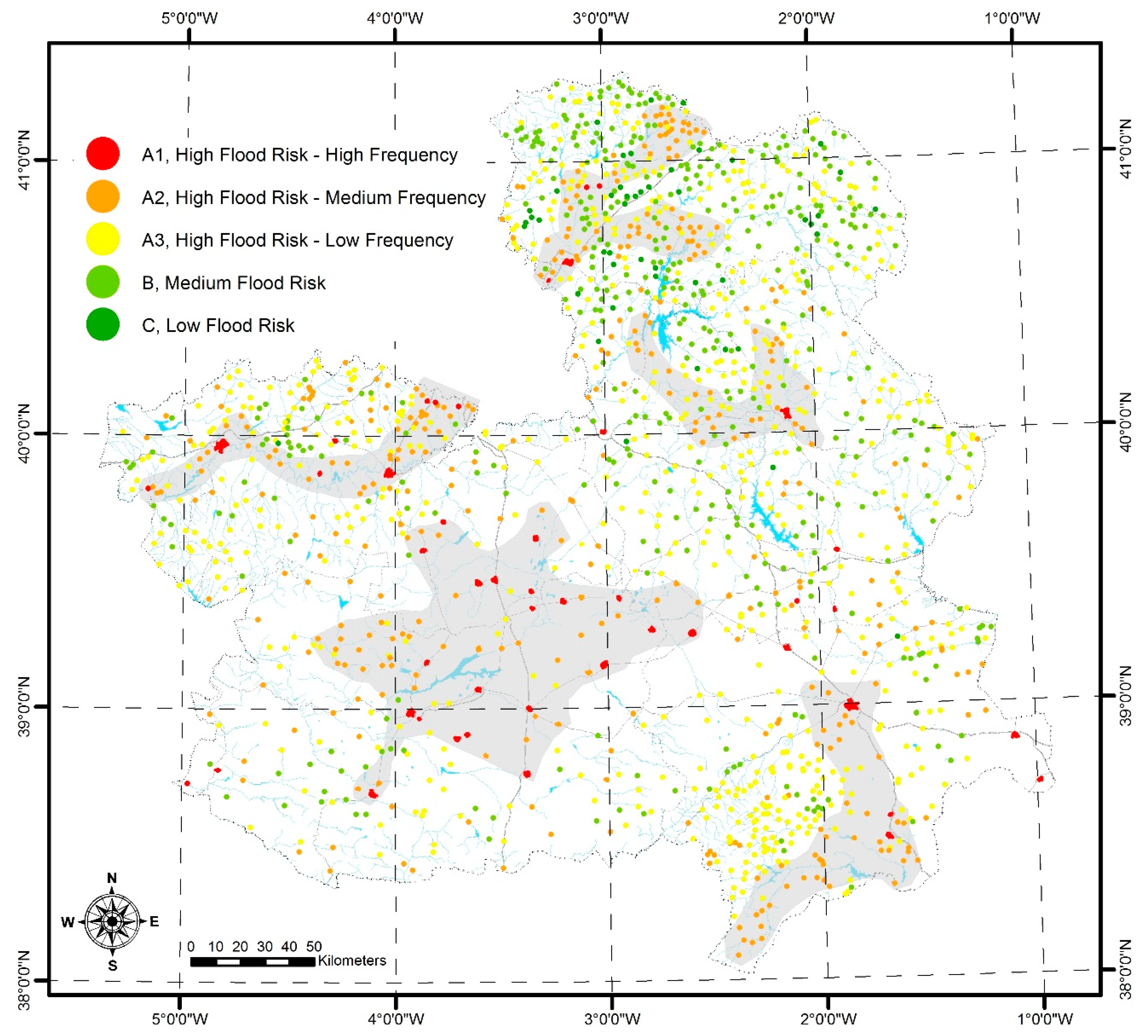
The results of the spatial MCA process allowed us to differentiate those population centers with a greater potential social flood risk. Thus, of the 1489 entities analyzed, 49 (3.4%) of them were assigned a maximum risk (A1), 371 (24.9%) were considered high risk (category A2), 605 (40.6%) were medium risk (A3), 417 (28%) were low risk (B), and 47 (3.1%) were assigned a very low risk (C).
Based on the results from the flood risk analysis, a proposal was made for population centers to identify hot-spots with the objective of prioritizing the development of local flood risk mitigation plans. It should be kept in mind that there will always be a priority for action by those population centers classified within risk groups A1 and A2. However, based on proximity and spatial concentration, five areas were delimited (Figure 4):
- The so-called “La Mancha” area,
- Southeast area of the province of Albacete,
- East Zone of the province of Guadalajara,
- Axis of the Tagus River in the province of Toledo,
- Areas surrounding the city of Cuenca.
Another important result was the high flood risk level of the main population centers of the autonomous community of Castilla-La Mancha. Out of the 62 populations that exceed the 5000 inhabitants threshold, almost 70% were classified with a maximum risk level (A1).
3.2. The Quality Assessment of Flood Risk Analysis (Phone Calls and LOESS)
As stated in the Introduction, the quality assessment of risk analysis and cartography as a potential situation is not easy. In the present study, we opted for the use of telephone calls to the Emergency Services during the seven years after the risk analysis ended (2007–2013). The data were analyzed using advanced statistical methods.
The set of baseline data used in this study was that provided by the Public Emergency Service 112 of the Castilla-La Mancha region. The service’s mission is to provide effective and coordinated help through the emergency number 112 in situations of emergency that may endanger people’s lives, the environment, property, rights, and the heritage of this region. The information contained in the records of the 112 Service is very basic for each phone call: identifier, date and time, municipality and province, and cause of the emergency (fire, flood, etc.). The dataset used corresponded to the calls received (only related to flooding processes) in the seven years after the completion of the risk analysis (year 2007), which amounted to around 17,000 phone calls distributed as shown in Table 3.
The statistical function LOESS [47,48] consists of a locally weighted regression to moderate a set of baseline data. The function attempts to smooth data to generate scatter diagrams.
The purpose of local regression is to create a trend line starting with a point cloud and taking into account the vicinity of the data to minimize the error. The algorithm is iterative and does not generate a function. It has the following parameters: bandwidth (h), which acts as a smoothing coefficient, and the polynomial degree used in interpolation. When performing a local regression, a parametric family is used as in a global regression adjustment, but the adjustment is only performed locally.
In practice, certain assumptions are made: (i) regression, continuity, and derivability are assumed, thus it can be well approximated by polynomials of a certain degree; (ii) for the variability of Y around the curve, for example, a constant variability is assumed.
The estimation methods that result from this type of models are relatively simple: (i) for each point x, an environment is defined; (ii) within that environment, we assume that a regressor function is approximated by some member of the parametric family that would be quadratic polynomials; (iii) the parameters are then estimated using contour data; (iv) the local adjustment is that of the adjusted function evaluated at x.
Generally, a weight function, W, is incorporated to give greater weight to the xi values that are close to x. Estimation criteria depend on the assumptions made about the distribution of the Y’s. If, for example, we assume that they have a Gaussian distribution with constant variance, it makes sense to use the least squares method.
The point cloud for which one wants to use LOESS is expressed as:
For example, use a third-degree polynomial that is expressed as:
In general, a polynomial of degree p can be expressed as:
where ak is the coefficient that must be solved to interpolate the value of x through local regression. To calculate the value of the coefficient ak, the following formula can be used:
in which X is the design matrix, where:
In the case of the third-degree polynomial that is being used as an example:
W is a diagonal matrix where each value assigns a weight:
The matrix Y simply represents the y coordinates of the input data:
The LOESS model in this study (source code for LOESS model is available as a Supplementary File) was applied using the R working environment. R is a free software environment for statistical computing that is widely used in academic and scientific fields (i.e., [49]) and which was created by Robert Gentleman and John Chambers in the Bell laboratories [50]. The degree of adjustment between the risk values and the number of phone calls defined both the statistical capacity of simulating the phenomena of the LOESS model and its usefulness for the validation of the analysis and the flood risk cartographies. Additionally, a positive correlation between the risk level of each municipality (according to MCA) and the number of calls to the Emergency Services (112) would show the usefulness of the analysis of 112 calls as a method for calibrating potential risk cartographies.
4. Results: Correlation Risk Categories vs. Number of Phone Calls
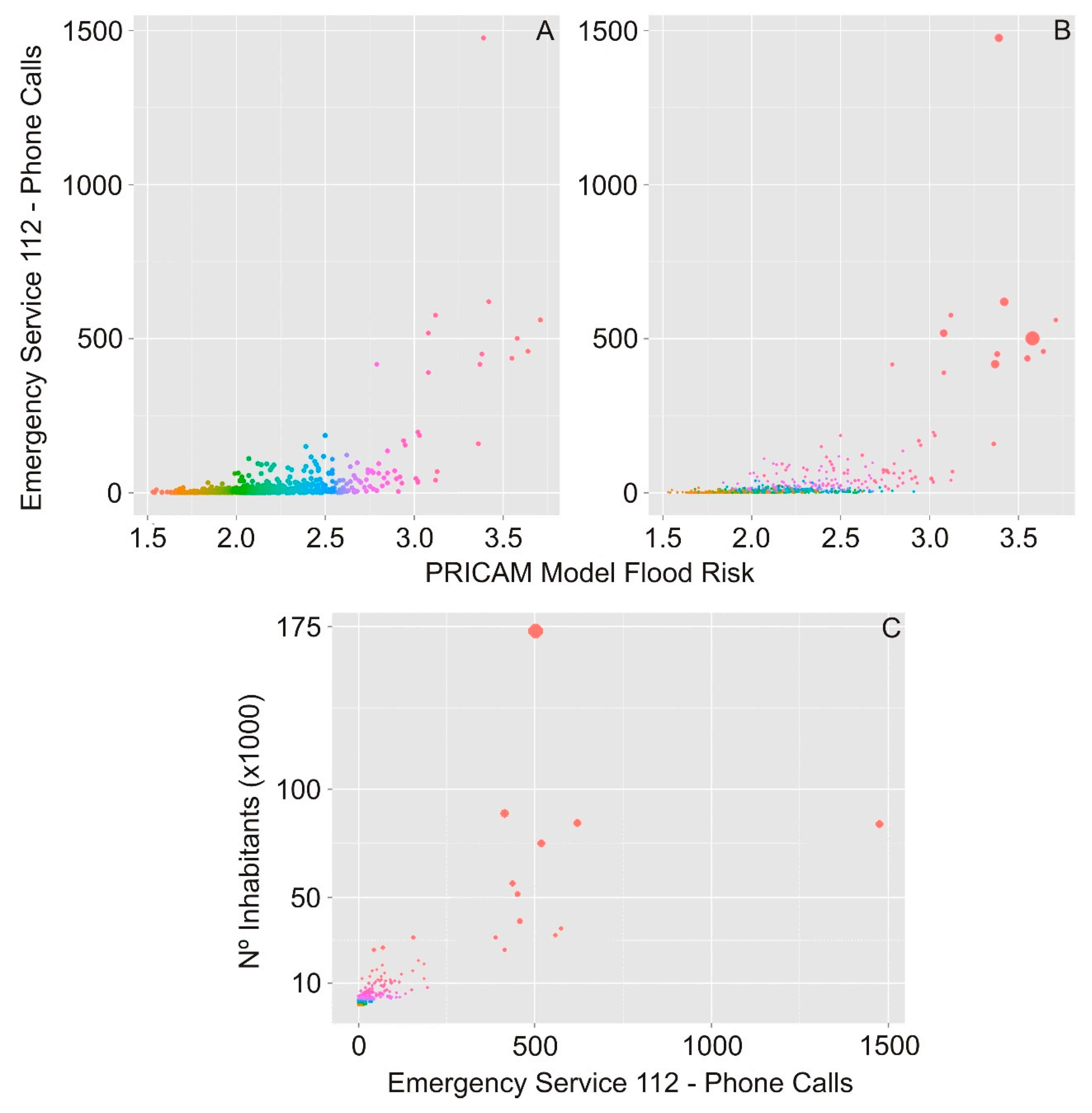
The combination of information and data sources used in this study allowed us firstly to describe the relationship between these variables as flood risk–population–emergency calls. As would be expected (and as shown in Figure 5), a positive relationship could be established between the variables considered both in the flood risk–emergency calls relationship and in the population–emergency calls relationship. However, even if there was a positive (and expected) relationship between these variables, the presence of values (corresponding to municipalities) that did not fit perfectly in this relation was observed. Those populations stood out that seemed to present a number of calls greater than what was expected for their assigned risk and population.
In addition to this descriptive analysis, the LOESS model also provided a detailed analysis of the relationship between the pairs of variables considered. This analysis allowed us to relate the flood risk value established from the MCA analysis (PRICAM project) with respect to the inferred risk value established from the LOESS statistical model. When applying the LOESS model using R, a table was obtained in which, for each municipality, a new risk value was inferred using the population of each locality as a major reason for the adjustment. In this table, one could see the municipalities for which there was a greater difference between the categorized risk and the inferred risk. A municipality appearing above or below the LOESS trend line in the LOESS graph indicated the need for a categorized risk review. The points above the trend line indicated that the categorized risk was greater than the inferred one, and the opposite situation was indicated for those that were below it.
Although the regression analysis gave good results, the presence of municipalities with a very high number of records (phone calls) controlled the shape of the local regression function in such a way that the municipalities with the highest number of calls presented extreme risk values that were much higher than the values from the PRICAM model. The highest value of the inferred risk obtained through the local regression function was 4.96, whereas it was only 3.64 from the PRICAM model.
A non-systematic search of incidents and information (from newspapers, reports, and field visits) on these municipalities showed that they were places in which episodes of floods were periodically recorded with important consequences for people and assets. Thus, high flood risk values were justified. It could be concluded that these inferred flood risk values should not be understood as a new flood risk assignment but as a starting point for the review of the PRICAM model flood risk database and its cartography on a risk map.
The inferred flood risk value for municipalities with a lower number of phone calls was very similar to those collected in the PRICAM. For municipalities with a record of incidences below 300 calls, the LOESS graph had a very high positive slope, thus it was understood that the inferred risk grew according to the calls, which indicated a good correlation between the calls and the value of the risk.
An inferred flood risk value lower than the categorized risk (PRICAM model) could also be used as a starting point in the PRICAM update process, since it indicated that the consequences of floods may have been neglected in these urban centers.
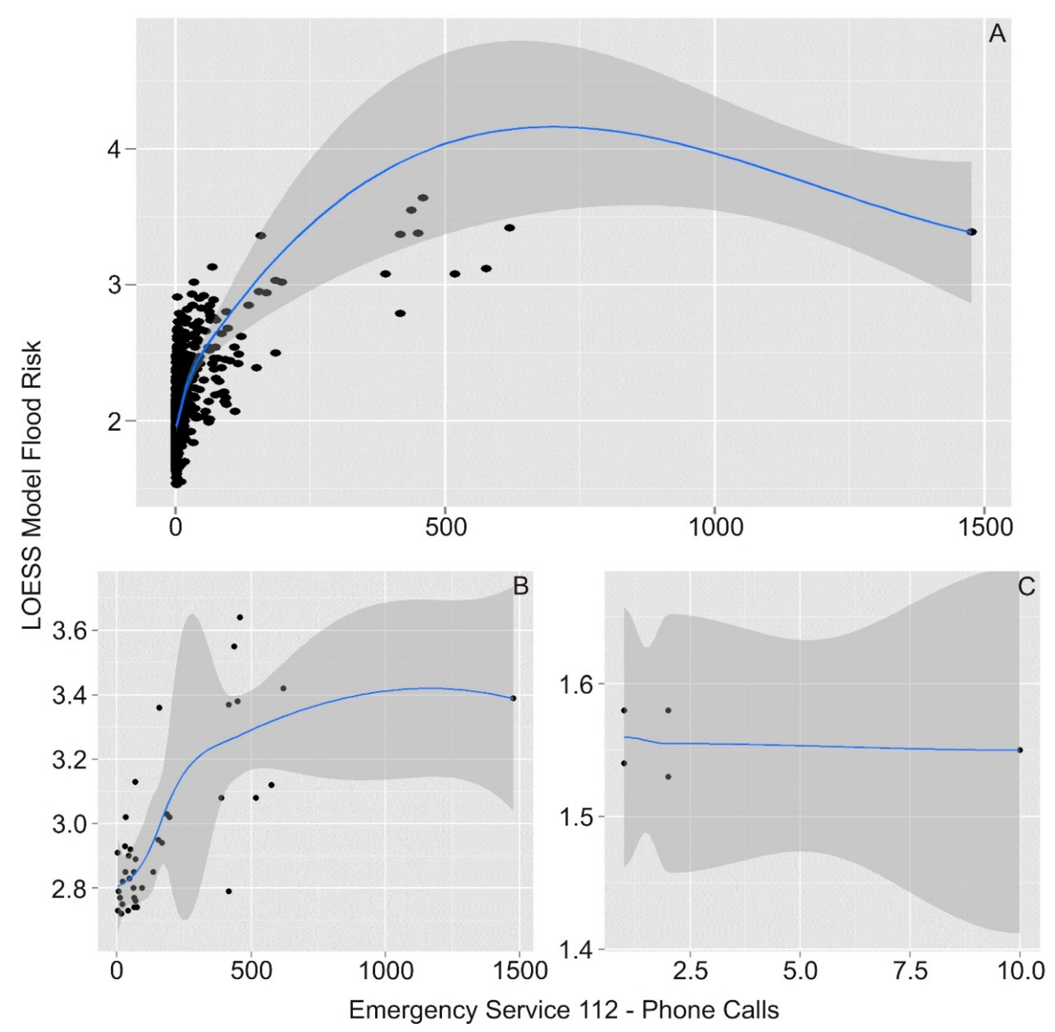
As the PRICAM model classified each urban center into one of the five risk categories used by Civil Protection regulations (A1, A2, A3, B, and C), a local regression trend could be established for each class using LOESS. In this way, the degree of correlation between the variables (emergency phone calls and flood risk) could be inferred for each level of risk considered (Figure 6). Figure 6 shows that the best correlation was established for the urban centers of flood risk group A1, since the higher the number of calls corresponded to higher risk value. In any of the other groups, the slope of the graph remained mainly constant, indicating a low correlation between the number of calls and the risk, which may have also indicated that the number of flood events collected was insufficient to establish the relationship between phone calls and risk.
For the regression trend by flood risk level, the local regression function no longer generated inferred risk values greater than those contemplated in the PRICAM model and even showed values below these.
For the municipalities of flood risk classes B and C, there were two situations to consider— the number of urban centers in these classes was very small, and the number of phone calls was also scarce. In these cases, LOESS assigned all municipalities a very similar risk value (which occurred in class C), or the dispersion between the value of the risk categorized and the one inferred was very small, thus there was hardly any difference.
5. Discussion
5.1. Data Sources and Methodological Limitations
The methodological proposal developed for the analysis of flood risk in the civil protection plan of Castilla-La Mancha solved, in an imaginative or an innovative way, the initial limitations and the difficulties derived from the limited availability of both cartographic and alphanumeric data. This point limited the variables that could be considered and the conditions implemented using the Delphi Fuzzy method for selection and weighting. Therefore, for its application to other spatial areas, the variables that could be used should be reconsidered by adapting them to the particularities of the study area.
Flood risk analyses that present a macro-scale approach generally imply some simplification in the analysis model, either in the hazard estimation [2] or the exposed elements [51], in order to make their development viable. In the potential flood risk PRICAM analysis model, floods affect the population as a whole, not subsets of it. This is due to not knowing the extension of the water surface and because the spatial resolution of socio-economic information would not allow it.
Therefore, the results derived from the PRICAM project would define a maximum potential flood risk for urban centers, which could differ (being generally greater) from the real flood risk obtained from micro-scale approaches [4,5,6,52]. However, according to the main objective of the study (potential flood risk ranking of urban centers as a criterion for the development of their local plan against flood risk), the deviations in the estimation of the real flood risks due to analysis simplification should not condition the validity of the analysis [2].
Beyond these limitations and simplifications, any risk analysis implies a certain subjectivity that depends on the method chosen or the variables analyzed. In the PRICAM project, a combination of MCA and GIS was chosen for flood risk analysis [53]. The choice of this model was based on considerations such as the type and the quality of the data available, the extent of the study area, or the type of result expected by the model. This choice was made despite the fact that, in most case studies, the MCA-GIS combination has been used more to evaluate flood risk mitigation measures than for risk mapping itself [35]. Perhaps the main source of subjectivity in the results obtained from an MCA is associated with the choice and the weighting of the variables used [35,54]. To limit this subjectivity, a Delphi Fuzzy model was used in such a way that the criteria that governed the MCA were based on the consensus among a national and multidisciplinary team of flood risk experts and the fact that the convergence of the experts’ criterion was reasonable.
The level of aggregation of socio-economic data can condition flood risk assessments (through its exposure and vulnerability components) based on MCA models and can thus bring about the assignment of high-risk levels that are associated with main urban areas. This effect can be found fundamentally when aggregation reaches municipality or urban center levels. This relationship would be based on considerations such as:
- High exposure linked to the total number of people in the urban center,
- High exposure linked to population density,
- High exposure linked to the presence of educational institutions, tourist camps, nursing homes, hospitals, or industrial estates,
- High vulnerability linked to the presence of children,
- High vulnerability linked to the presence of patients or convalescents (hospitals),
- Most of these major urban areas are historically developed close to rivers, thus the hazard factor (according to the characteristics of the model used) will also show a high value.
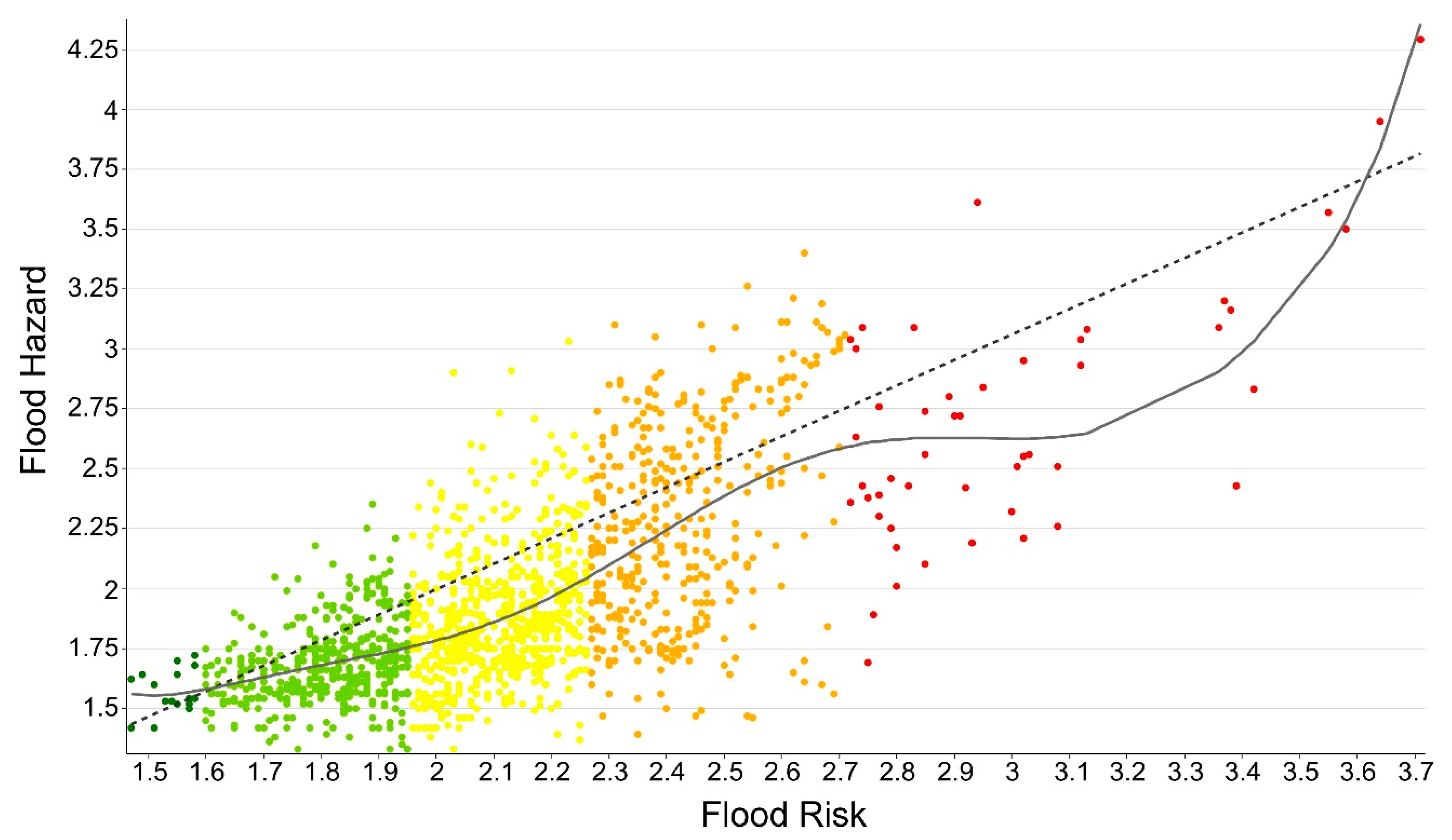
The situation described above could be considered as a bias in the results obtained. The clearest example of this effect is found if we analyze those urban centers classified as an A1 flood risk. Out of the total 1489 urban centers, only 49 reached that level of risk, and 43 of these 49 urban centers could be considered as “major towns”. Therefore, the following conclusion could be reached—the results of the MCA model of flood risk analysis magnify the level of risk in the main urban centers, underestimating the role of the flooding hazard in the obtained results. However, after a more in-depth analysis, this statement loses its validity. Let us start with one data item; from the 1489 urban centers, only 31 were classified with the maximum level of flood hazard. Out of those 31 populations, only one obtained a flood risk assessment lower than A2. As regards the other 30 urban centers, 13 were included in flood risk level A1, and the remaining 17 were in flood risk level A2. From these results, another (perhaps more realistic) conclusion could be drawn regarding the results of the analysis—the flood hazard played an equal role in the whole flood risk analysis, as can be seen in the figure relating both variables (Figure 7). Those urban centers that presented high values of flood hazard were finally included in the high or the extreme flood risk classes.
Another point of the PRICAM model with which a certain degree of subjectivity could be associated was the urban center flood risk classification into the Basic Civil Protection Directive flood risk levels of Spain. This classification was based on the opinion of the experts involved in the development of the PRICAM model from descriptive and graphical statistical analyses (Figure 3 and Figure 7) of the results of the project. Similar approaches to the assessment and the management of flood risk have been adopted for the flood risk management policy in countries such as the United Kingdom, Austria, and Germany [55].
Regarding the LOESS function used to approach a calibration method for the analysis of potential flood risk from phone calls to the Emergency Service (112), it was observed that an individual flood risk level analysis was necessary. The conclusion came from visual analysis of the graphs showing the number of calls and the flood risk. When all flood risk levels were included without any discrimination, unexpected results were obtained in such a way that the greater value of the inferred risk (the one obtained through the local regression fit) was much higher than the maximum value of flood risk collected for any urban center in the PRICAM model. Therefore, the error estimated by the regression model was very high.
In a second approach, it was decided to use the flood risk classes of the Basic Civil Protection Directive of Spain—those that differentiated urban centers into A1, A2, A3, B, and C levels. As expected, the largest number of phone calls was concentrated on the first classes, which suffered more flooding events. By focusing on the analysis of these flood risk levels, more accurate analyses were achieved, the local regression trend worked much better, and estimated errors were smaller.
For any of the risk levels, analysis of flood risk validation required filtering the phone calls to the 112 service. This was due to the fact that, in urban centers for which only one or two flood events were registered in the time period analyzed (2007–2013), very few phone calls could imply “noise” that altered the regression model and did not contribute valuable data. In this sense, as proposed by Calle et al. [49] for the generation of longitudinal profiles of rivers and the adjustment of historical precipitation trends, the application of the LOESS function could limit the “noise” generated by small anomalies in the variable analyzed.
Although the above could be considered as a bias in the spatio-temporal distribution of data associated with 112 phone calls, the magnitude and the importance of this bias were not comparable to those currently associated with the use of citizen or crowd-source data [30,56], which is higher by one or two orders of magnitude. On the other hand, the use of citizen sources is more common in studies focused on natural hazards assessment (disasters detection and real time monitoring), not for integrated risk assessment (including damages and losses). This circumstance may be due to the need for element vulnerability (elements fragility) when we consider the existence of risk. Additionally, in these situations, the population tends to contact those agencies in charge of emergency management more than social or citizen projects and networks.
Moreover, the study time period (seven years) seemed insufficient, since the frequency of flood events in many of the urban centers analyzed was less than the time range covered by the used phone call dataset. However, this methodological approach could be a good starting point to determine which urban centers should be considered for PRICAM model reviews. The criteria for doing the reviews can be considered as follows:
- Urban centers for which the value of the inferred flood risk (LOESS regression trend) is greater than that of the categorized risk (PRICAM model); in these urban centers, flooding events have registered consequences on people and/or assets that result in a high number of phone calls to the Emergency Service 112.
- Urban centers with a value of inferred flood risk lower than the categorized risk; in these situations, there have not been enough flooding events to justify flood risk classifications greater than those inferred by LOESS.
5.2. Future Applications
Due to the impossibility of calibrating and validating the results of an analysis of potential flood risk over large areas due to the innumerous exposed elements and their different vulnerabilities, it is necessary to search for methodologies that allow us to implement post-analysis calibration measures. In order to achieve these goals, the use of information derived from social (or citizen) networks is generalized in the process of calibrating the hazard level (less for risk characterization) posed by different natural phenomena [19,20,21,22,23,24,25,26,27]. However, it has been observed that the use of data from social networks has its disadvantages [28,29,30]. From the results of other recent studies [56], a bias in crowd-source data availability and spatial distribution could be denoted, even in projects that enjoyed an important degree of maturity, as in the case of the CrowdHydrology project in the USA. In this sense, the use of information from Emergency Services solves some of these weak points, such as the different degree of implementation and the use of social networks based on age, gender, and location (rural or urban environment). In spite of the above, it is evident that the joint use of official and crowd-source data must be developed and improved in the coming years, and it can and should be the future trend for the validation of natural hazard and risk assessments.
However, data collected from phone calls to Emergency Services are also limited (and require a multi-year period of data collection to be considered significant), as they do not collect information regarding the severity of the flood event, the exposed elements affected, or the degree of damage suffered by them. In this sense and with the aim of achieving the best possible calibration of potential flood risk cartographies, we may have to focus our efforts on the implementation and/or the detailed study of the reports generated by Territorial Intervention Units in the territory with the flood risk, mainly formed in Spain by the Civil Guard (SEPRONA), local police, fire departments, and Civil Protection Units. Thus, reports generated in the field by the intervention units can respond to the uncertainties associated with the severity of the phenomenon or the elements affected by it. The use of this type of information together with local regression models (such as the LOESS model used in the present study) should allow better calibration of the studies of potential flood risk as well as prioritization based on scientific criteria of the more detailed studies (meso- and micro-scale).
5.3. Map Update
Regarding the flood risk analysis, the most important updates and those that should be made more frequently are those related to the determination of exposure and vulnerability of the population. The variables that take into account characteristics of the buildings, as well as some related to the population (e.g., civil status, economic activity) are only updated every ten years in the case of the Spanish official Census of the Population. The variables linked to the basic characteristics of the population (age, sex, nationality, level of studies) may have a much higher update frequency, since they are included in the Municipal Register, which is constantly updated. However, because the record-keeping systems are non-standard, using the 919 available municipal registers seems to be unfeasible from the point of view of methodology and the time needed.
Regarding the variables associated with flood hazard, the optimal update frequency tends to prefer a 10-year review rather than a continuous update. The updating of peak flows (or rainfall) associated with different return periods based on a series of instrumental measures regarding annual maximum peak flows should not show significant variations (for the proposed frequency update), even in the global climate change scenario.
The development or the general acceptance of new techniques or methodologies for the validation and the calibration of flood risk should at least be taken into account for their use in the next scheduled update. In any case, in the field of flood risk analysis at a regional or a national scale, the implementation of a program of regular model updates should be considered as the fourth axis on which the risk analysis is based.
6. Conclusions
A new proposal was presented for the calibration and the validation of flood risk maps at a regional, a national, or even a supra-national scale based on information derived from phone calls to the Emergency Service (112) of the autonomous community of Castilla-La Mancha (Spain) and the use of local regression models such as LOESS. Within this methodological framework, the LOESS model establishes the relationship between the number of calls to the Emergency Service and the categorized flood risk level derived from the PRICAM project.
The results obtained in the study show the usefulness of the data provided by citizen collaboration (calls to the emergency telephone number) in the process of calibration of flood risk analysis and maps. Since this calibration process is not biased by the socio-economic factors of the population, the limiting calibration factor depends on the volume of data available (which are limited by the period of time elapsed after completion of the flood risk analysis).
When the local regression model (LOESS) used the total number of calls to the Emergency Service, it was observed that the model overestimated the potential risk value defined within the PRICAM project, mainly in those populations with the highest number of phone calls. However, these differences between categorized and inferred risk values did not modify the hierarchical order of municipalities according to the level of risk, thus they remained valid in their prioritization. When regression trends were calculated on subsets of calls (defined by the flood risk level of urban centers in the PRICAM model), the differences disappeared between categorized and inferred flood risk; moreover, no change in the layout of urban centers with respect to their flood risk level was observed.
These results highlight two main ideas; on the one hand, the estimation of the flood risk level carried out in the PRICAM project (combining Fuzzy DELPHI, MCA, and GIS techniques) can be considered optimal for a national scale analysis. On the other hand, the application of statistical models of local regression on data collected in the regional or the national Emergency Services will serve to improve the processes of calibration and validation of potential flood risk cartographies. It also allows us to prioritize urban centers for the development of flood risk analysis at regional or local scales.
Supplementary Materials
The following are available online at https://www.mdpi.com/2073-4441/11/6/1284/s1.
Author Contributions
All authors have a significant contribution to final version of the paper. Conceptualization, J.G. and A.D.-H.; Flood risk analysis, J.G. and A.D.-H.; LOESS analysis, I.G.-P. and A.D.-H.; Writing—original draft, J.G. and A.D.-H.; Writing—review & editing, all authors.
Funding
This research was funded by the project DRAINAGE, CGL2017-83546-C3-R (MINEICO/AEI/FEDER, UE), and it is specifically part of the assessments carried out under the coverage of the sub-project DRAINAGE-3-R (CGL2017-83546-C3-3-R).
Acknowledgments
The authors would like to thank the following administrations for their collaboration: the Civil Protection Service, 112, and the General Directorate for Citizen Protection of the Regional Government of Castilla-La Mancha; the Statistical Institute of Castilla-La Mancha; to the Geological Survey of Spain (IGME); and to all the staff of experts who collaborated in the Fuzzy DELPHI analysis. Part of the present manuscript constituted the Master Thesis of the second of the authors, presented in the Master in Evaluation and Management of the Geographic Information Quality of the University of Jaén (Spain).
Conflicts of Interest
The authors declare no conflict of interest.
References
- Centre for Research on the Epidemiology of Disasters. The International Disaster Database. Available online: http://emdat.be/emdat_db/ (accessed on 10 October 2018).
- De Moel, H.; Jongman, B.; Kreibich, H.; Merz, B.; Penning-Rowsell, E.; Ward, P.J. Flood risk assessments at different spatial scales. Mitig. Adapt. Strateg. Glob. Chang. 2015, 20, 865–890. [Google Scholar] [CrossRef] [PubMed] [Green Version]
- Sayers, P.; Lamb, R.; Panzeri, M.; Bowman, H.; Hall, J.; Horritt, M.; Penning-Rowsell, E. Believe it or not? The challenge of validating large scale probabilistic risk models. In Proceedings of the FLOODrisk 2016, Lyon, France, 17–21 October 2016. [Google Scholar]
- Evans, E.P.; Johnson, P.J.; Green, C.H.; Varsa, E. Risk assessment and programme prioritisation: The Hungary flood study. In Proceedings of the 35th Annual MAFF Conference of River and Coastal Engineers, London, UK, July 2000. [Google Scholar]
- Cook, A.; Merwade, V. Effect of topographic data, geometric configuration and modeling approach on flood inundation mapping. J. Hydrol. 2009, 377, 131–142. [Google Scholar] [CrossRef]
- Penning-Rowsell, E.C. A realistic assessment of fluvial and coastal flood risk in England and Wales. Trans. Inst. Br. Geogr. 2015, 40, 44–61. [Google Scholar] [CrossRef]
- Penning-Rowsell, E.C. A ‘realist’ approach to the extent of flood risk in England and Wales. In Comprehensive Flood Risk Management: Research for Policy and Practice; Klijn, F., Schweckendiek, T., Eds.; Taylor and Francis: London, UK, 2013. [Google Scholar]
- Dottori, F.; Salamon, P.; Bianchi, A.; Alfieri, L.; Hirpa, F.A.; Feyen, L. Development and evaluation of a framework for global flood hazard mapping. Adv. Water Resour. 2016, 94, 87–102. [Google Scholar] [CrossRef]
- McCallum, I.; Liu, W.; See, L.; Mechler, R.; Keating, A.; Hochrainer-Stigler, S.; Mochizuki, J.; Fritz, S.; Dugar, S.; Arestegui, M.; et al. Technologies to support community flood disaster risk reduction. Int. J. Disaster Risk Sci. 2016, 7, 198–204. [Google Scholar] [CrossRef]
- Pappenberger, F.; Beven, K.; Frodsham, K.; Romanowicz, R.; Matgen, P. Grasping the unavoidable subjectivity in calibration of flood inundation models. A vulnerability weighted approach. J. Hydrol. 2007, 333, 275–287. [Google Scholar] [CrossRef]
- Zischg, A.P.; Mosimann, M.; Bernet, D.B.; Röthlisberger, V. Validation of 2D flood models with insurance claims. J. Hydrol. 2018, 557, 350–361. [Google Scholar] [CrossRef] [Green Version]
- Alfonso, L.; Lobbrecht, A.; Price, R. Using mobile phones to validate models of extreme events. In Proceedings of the 9th International Conference on Hydroinformatics, Tianjin, China, 7–11 September 2010; pp. 1447–1454. [Google Scholar]
- Poser, K.; Dransch, D. Volunteered geographic information for disaster management with application to rapid flood damage estimation. Geomatica 2010, 64, 89–98. [Google Scholar]
- Hung, K.C.; Kalantari, M.; Rajabifard, A. Methods for assessing the credibility of volunteered geographic information in flood response: A case study in Brisbane, Australia. Appl. Geogr. 2016, 68, 37–47. [Google Scholar] [CrossRef]
- Le Coz, J.; Patalano, A.; Collins, D.; Guillén, N.F.; García, C.M.; Smart, G.M.; Bind, J.; Chiaverini, A.; Le Boursicaud, R.; Dramais, G.; et al. Crowd-sourced data for flood hydrology: Feedback from recent citizen science projects in Argentina, France and New Zealand. J. Hydrol. 2016, 541, 766–777. [Google Scholar] [CrossRef]
- Rollason, E.; Bracken, L.J.; Hardy, R.J.; Large, A.R.G. The importance of volunteered geographic information for the validation of flood inundation models. J. Hydrol. 2018, 562, 267–280. [Google Scholar] [CrossRef]
- Montargil, F.; Santos, V. Citizen observatories: Concept, opportunities and communication with citizens in the first EU experiences. In Beyond Bureaucracy: Towards Sustainable Governance Informatisation; Paulin, A.A., Anthopoulos, L.G., Reddick, C.G., Eds.; Springer International Publishing: Cham, Switzerland, 2017; pp. 167–184. [Google Scholar]
- Assumpção, T.H.; Popescu, I.; Jonoski, A.; Solomatine, D.P. Citizen observations contributing to flood modelling: Opportunities and challenges. Hydrol. Earth Syst. Sci. 2018, 22, 1473–1489. [Google Scholar] [CrossRef]
- Schnebele, E.; Cervone, G. Improving remote sensing flood assessment using volunteered geographical data. Nat. Hazards Earth Syst. Sci. 2013, 13, 669–677. [Google Scholar] [CrossRef] [Green Version]
- Triglav-Čekada, M.; Radovan, D. Using volunteered geographical information to map the November 2012 floods in Slovenia. Nat. Hazards Earth Syst. Sci. 2013, 13, 2753–2762. [Google Scholar] [CrossRef] [Green Version]
- Smith, L.; Liang, Q.; James, P.; Lin, W. Assessing the utility of social media as a data source for flood risk management using a real-time modelling framework. J. Flood Risk Manag. 2015, 10, 370–380. [Google Scholar] [CrossRef]
- Cervone, G.; Sava, E.; Huang, Q.; Schnebele, E.; Harrison, J.; Waters, N. Using Twitter for tasking remote-sensing data collection and damage assessment: 2013 Boulder flood case study. Int. J. Remote Sens. 2016, 37, 100–124. [Google Scholar] [CrossRef]
- Li, Z.; Wang, C.; Emrich, C.T.; Guo, D. A novel approach to leveraging social media for rapid flood mapping: A case study of the 2015 South Carolina floods. Cartogr. Geogr. Inf. Sci. 2017, 45, 97–110. [Google Scholar] [CrossRef]
- Starkey, E.; Parkin, G.; Birkinshaw, S.; Large, A.; Quinn, P.; Gibson, C. Demonstrating the value of community based (“citizen science”) observations for catchment modelling and characterization. J. Hydrol. 2017, 548, 801–817. [Google Scholar] [CrossRef]
- Kusumo, A.N.L.; Reckien, D.; Verplanke, J. Utilising volunteered geographic information to assess resident’s flood evacuation shelters. Case study: Jakarta. Appl. Geogr. 2017, 88, 174–185. [Google Scholar] [CrossRef]
- Kryvasheyeu, Y.; Chen, H.; Obradovich, N.; Moro, E.; Van Hentenryck, P.; Fowler, J.; Cebrian, M. Rapid assessment of disaster damage using social media activity. Sci. Adv. 2016, 2, e1500779. [Google Scholar] [CrossRef] [PubMed]
- Goodchild, M.F.; Glennon, J.A. Crowdsourcing geographic information for disaster response: A research frontier. Int. J. Digit. Earth 2010, 3, 231–241. [Google Scholar] [CrossRef]
- Rosser, J.F.; Leibovici, D.G.; Jackson, M.J. Rapid flood inundation mapping using social media, remote sensing and topographic data. Nat. Hazards 2017, 87, 103–120. [Google Scholar] [CrossRef] [Green Version]
- Goodchild, M.F.; Li, L. Assuring the quality of volunteered geographic information. Spat. Stat. 2012, 1, 110–120. [Google Scholar] [CrossRef]
- Xiao, Y.; Huang, Q.; Wu, K. Understanding social media data for disaster management. Nat. Hazards 2015, 79, 1663–1679. [Google Scholar] [CrossRef]
- Fernández-García, F. El Clima de la Meseta Meridional. Los Tipos de Tiempo; Universidad Autónoma de Madrid: Madrid, Spain, 1985; 215p. [Google Scholar]
- Instituto Nacional de Meteorología. Guía Resumida del Clima en España 1971—2000; INM: Madrid, Spain, 2001. [Google Scholar]
- Díez-Herrero, A.; Garrote, J.; Baillo, R.; Laín, L.; Mancebo, M.J.; Pérez-Cerdán, F. Análisis del riesgo de inundación para planes autonómicos de protección civil: RICAM. In El Estudio y la Gestión de Los Riesgos Geológicos; Jiménez, I.G., Huerta, L.L., Isidro, M.L., Eds.; Instituto Geológico y Minero de España: Madrid, Spain, 2008; pp. 53–70. [Google Scholar]
- Ministerio de Justicia e Interior del Gobierno de España. Directriz básica de planificación de protección civil ante el riesgo de inundaciones. Boletín Oficial del Estado 1995, 38, 4846–4858. [Google Scholar]
- Meyer, V.; Scheuer, S.; Haase, D. A multicriteria approach for flood risk mapping exemplified at the Mulde river, Germany. Nat. Hazards 2009, 48, 17–39. [Google Scholar] [CrossRef]
- Brouwer, R.; van Ek, R. Integrated ecological, economic and social impact assessment of alternative flood control policies in the Netherlands. Ecol. Econ. 2004, 50, 1–21. [Google Scholar] [CrossRef]
- Akter, T.; Simonovic, S.P. Aggregation of fuzzy views of a large number of stakeholders for multiobjective flood management decision-making. J. Environ. Manag. 2005, 77, 133–143. [Google Scholar] [CrossRef]
- Raaijmakers, R.; Krywkow, J.; van der Veen, A. Flood risk perceptions and spatial multi-criteria analysis: An exploratory research for hazard mitigation. Nat. Hazards 2008, 46, 307–322. [Google Scholar] [CrossRef]
- Huang, D.; Zhang, R.; Huo, Z.; Mao, F.; Youhao, E.; Zheng, W. An assessment of multidimensional flood vulnerability at the provincial scale in China based on the DEA method. Nat. Hazards 2012, 64, 1575–1586. [Google Scholar] [CrossRef]
- Li, C.H.; Li, N.; Wu, L.D.; Hu, A.J. A relative vulnerability estimation of flood disaster using data envelopment analysis in the Dongting Lake region of Hunan. Nat. Hazards Earth Syst. Sci. 2013, 13, 1723–1734. [Google Scholar] [CrossRef]
- Balica, S.F.; Popescu, I.; Beevers, L.; Wright, N.G. Parametric and physically based modelling techniques for flood risk and vulnerability assessment: A comparison. Environ. Model. Softw. 2013, 41, 84–92. [Google Scholar] [CrossRef]
- Linstone, H.A.; Turrof, M. The Delphi Method. Techniques and Applications; Addison-Wesley Educational Publishers Inc.: Boston, MA, USA, 1975; 621p. [Google Scholar]
- Landeta, J. El Método Delphi. Una Técnica de Previsión Para la Incertidumbre; Ariel: Barcelona, Spain, 1999; 223p. [Google Scholar]
- Nasiri, H.; Yusof, M.J.M.; Ali, T.A.M.; Hussein, M.K.B. District flood vulnerability index: Urban decision-making tool. Int. J. Environ. Sci. Technol. 2018, 16, 2249–2258. [Google Scholar] [CrossRef]
- Ministerio de Fomento. Máximas Lluvias Diarias en la España Peninsular; Ministerio de Fomento de España: Madrid, Spain, 1999; 54p, (include software program MaxPluWin).
- Instituto Geológico y Minero de España. Geological and Geomorphological Map of Spain. Available online: http://info.igme.es/cartografiadigital/portada/default.aspx?mensaje=true (accessed on 20 September 2018).
- Cleveland, W.S. Robust locally weighted regression and smoothing scatterplots. J. Am. Stat. Assoc. 1979, 74, 829–836. [Google Scholar] [CrossRef]
- Cleveland, W.S.; Devlin, S.J. Locally weighted regression: An approach to regression analysis by local fitting. J. Am. Stat. Assoc. 1988, 83, 596–610. [Google Scholar] [CrossRef]
- Calle, M.; Alho, P.; Benito, G. Channel dynamics and geomorphic resilience in an ephemeral Mediterranean river affected by gravel mining. Geomorphology 2017, 285, 333–346. [Google Scholar] [CrossRef]
- R Development Core Team. R: A Language and Environment for Statistical Computing; R Foundation for Statistical Computing: Vienna, Austria, 2008. [Google Scholar]
- Merz, B.; Kreibich, H.; Schwarze, R.; Thieken, A. Review article “Assessment of economic flood damage”. Nat. Hazards Earth Syst. Sci. 2010, 10, 1697–1724. [Google Scholar] [CrossRef]
- Garrote, J.; Alvarenga, F.M.; Díez-Herrero, A. Quantification of flash flood economic risk using ultra-detailed stage—Damage functions and 2-D hydraulic models. J. Hydrol. 2016, 541, 611–625. [Google Scholar] [CrossRef]
- Malczewski, J. GIS-based multicriteria decision analysis: A survey of the literature. Int. J. Geogr. Inf. Sci. 2006, 20, 703–726. [Google Scholar] [CrossRef]
- Lee, G.; Jun, K.S.; Chung, E.S. Integrated multi-criteria flood vulnerability approach using fuzzy TOPSIS and Delphi technique. Nat. Hazards Earth Syst. Sci. 2013, 13, 1293–1312. [Google Scholar] [CrossRef] [Green Version]
- Thaler, T.; Hartmann, T. Justice and flood risk management: Reflecting on different approaches to distribute and allocate flood risk management in Europe. Nat. Hazards 2016, 83, 129–147. [Google Scholar] [CrossRef]
- Lowry, C.S.; Fienen, M.N.; Hall, D.M.; Stepenuck, K.F. Growing pains of crowdsourced stream stage monitoring using mobile phones: The development of crowdhydrology. Front. Earth Sci. 2019, 7, 128. [Google Scholar] [CrossRef]
Figure 1.
Location map of the autonomous community of Castilla-La Mancha. Dark blue circles show the location of each province capital city, and the black dots show the location of major towns.
Figure 1.
Location map of the autonomous community of Castilla-La Mancha. Dark blue circles show the location of each province capital city, and the black dots show the location of major towns.

Figure 2.
Diagram of the main variable groups used for the flood risk analysis of PRICAM project.

Figure 3.
Flood risk values histogram used for risk class thresholds delimitation into the flood risk analysis of the PRICAM project.
Figure 3.
Flood risk values histogram used for risk class thresholds delimitation into the flood risk analysis of the PRICAM project.

Figure 4.
Urban centers flood risk classification for autonomous community of Castilla-La Mancha. Grey shadow areas show the flood risk high values concentration areas.
Figure 4.
Urban centers flood risk classification for autonomous community of Castilla-La Mancha. Grey shadow areas show the flood risk high values concentration areas.

Figure 5.
Emergency Service 112 (phone calls) vs. PRICAM model flood risk values (A), with color dots size (B) showing urban centers population size. N° of Inhabitants vs. Emergency Service 112 phone calls (C), with color dots size showing urban centers population size.
Figure 5.
Emergency Service 112 (phone calls) vs. PRICAM model flood risk values (A), with color dots size (B) showing urban centers population size. N° of Inhabitants vs. Emergency Service 112 phone calls (C), with color dots size showing urban centers population size.

Figure 6.
Locally estimated scatterplot smoothing (LOESS) model fits for flood risk values vs. phone calls number (Emergency Service 112) for all flood risk classes (A), flood risk class A (B), and flood risk class C (C). Flood risk classes are from PRICAM project results.
Figure 6.
Locally estimated scatterplot smoothing (LOESS) model fits for flood risk values vs. phone calls number (Emergency Service 112) for all flood risk classes (A), flood risk class A (B), and flood risk class C (C). Flood risk classes are from PRICAM project results.

Figure 7.
Flood risk vs. flood hazard values from results of the PRICAM project. Dot colors (from dark green to red) show the flood risk class (from C to A1). Dashed line shows the linear regression fit for values. Solid line shows the 10th order polynomial regression fit for flood risk and flood hazard values.


Table 1.
List of variables used in PRICAM project and associated values of DELPHI analysis.
| Variable | Mean Value | Skewness | Kurtosis |
|---|---|---|---|
| Flooding probability: Qt to Qb ratio | 3.5;4.2;4.9 | −1.30 | 0.72 |
| Time of concentration (Tc) | 3.9;4.5;5.0 | −0.48 | −1.65 |
| Distance to river reach | 2.9;3.6;4.3 | −0.25 | −0.90 |
| Urban center–river reach elevation difference | 3.1;3.9;4.7 | −1.29 | 2.10 |
| Lithology and geomorphology sediments | 3.4;4.0;4.6 | −0.48 | −1.65 |
| Terrain slope | 3.6;4.1;4.6 | −0.26 | −1.12 |
| Terrain morphology (concave or convexity) | 3.7;4.2;4.7 | −0.44 | −1.23 |
| 24 h rainfall | 3.9;4.4;4.8 | −0.69 | −0.25 |
| Dam or reservoir class (volume) | 2.5;3.2;3.9 | −0.73 | 1.03 |
| Downstream distance from reservoir | 3.2;4.0;4.8 | −1.85 | 4.13 |
| N° of historical flood events | 4.0;4.5;4.9 | −0.69 | −0.25 |
| Historical vs actual reservoirs scenario | 3.2;3.8;4.4 | −0.67 | −0.10 |
| Toxic of danger materials industries | 3.4;4.1;4.8 | −1.07 | 0.37 |
| Industrial estate | 2.6;3.5;4.3 | −0.04 | −1.65 |
| Total population (number) | 3.8;4.5;5.1 | −2.05 | 4.83 |
| Population clustering by age | 2.8;3.4;3.9 | −0.85 | −0.76 |
| Unemployment index | 1.2;1.8;2.4 | 0.57 | −0.86 |
| Presence of educational institutions | 2.5;3.1;3.7 | 0.71 | 0.53 |
| Presence of hospital centers | 3.4;3.9;4.5 | −1.06 | 1.93 |
| Housing type | 3.0;3.9;4.8 | −1.25 | 1.26 |
| Under 6 year population ratio | 3.6;4.2;4.8 | −1.24 | 1.75 |
| Up 65 year population ratio | 3.8;4.4;4.9 | −1.58 | 2.78 |
| Presence of people with disabilities | 3.7;4.3;4.8 | −1.54 | 2.90 |
| Knowledge of the local language ratio | 2.0;2.8;3.6 | 0.20 | −0.81 |
| Presence of sick or convalescent people | 3.5;4.1;4.7 | −0.98 | 0.93 |
| Degree of buildings accessibility | 2.6;3.2;3.8 | −0.35 | −1.45 |
| State of buildings preservation | 2.9;3.6;4.3 | −0.27 | −0.65 |
| N° of stores above ground surface | 3.5;4.1;4.7 | −0.76 | 0.16 |
| N° of stores below ground surface | 4.3;4.7;5.2 | −1.64 | 1.13 |
| Distance to roads or evacuation paths | 2.8;3.5;4.3 | −0.51 | −0.92 |
| Distance to urban centers | 3.5;4.0;4.5 | −1.62 | 5.50 |
| Existence of defined evacuation paths | 4.4;4.7;5.0 | −0.81 | −1.65 |
Table 2.
Flood risk categories based on the Basic Directive for Civil Protection against Flood Hazards.
Table 2.
Flood risk categories based on the Basic Directive for Civil Protection against Flood Hazards.
| Risk Level | Description |
|---|---|
| A1 | High Frequency—High Flood Risk; 50-year flood produces significant damage to urban center |
| A2 | Medium Frequency—High Flood Risk; 100-year flood produces significant damage to urban center |
| A3 | Low Frequency—High Flood Risk; 500-year flood produces significant damage to urban center |
| B | Medium Flood Risk; 100-year flood produces significant damage outside the urban center |
| C | Low Flood Risk; 500-year flood produces significant damage outside the urban center |
Table 3.
Summary of phone calls received by the Emergency Service 112 of Castilla-La Mancha regarding floods.
Table 3.
Summary of phone calls received by the Emergency Service 112 of Castilla-La Mancha regarding floods.
| Year | Semester | N° Phone Calls |
|---|---|---|
| 2007 | 1 | 1943 |
| 2007 | 2 | 1101 |
| 2008 | 1 | 1062 |
| 2008 | 2 | 1730 |
| 2009 | 1 | 817 |
| 2009 | 2 | 2190 |
| 2010 | 1 | 1448 |
| 2010 | 2 | 1500 |
| 2011 | 1 | 1239 |
| 2011 | 2 | 584 |
| 2012 | 1 | 586 |
| 2012 | 2 | 951 |
| 2013 | 1 | 740 |
| 2013 | 2 | 825 |
| Total: | 16,828 | |
© 2019 by the authors. Licensee MDPI, Basel, Switzerland. This article is an open access article distributed under the terms and conditions of the Creative Commons Attribution (CC BY) license (http://creativecommons.org/licenses/by/4.0/).
Share and Cite
MDPI and ACS Style
Garrote, J.; Gutiérrez-Pérez, I.; Díez-Herrero, A. Can the Quality of the Potential Flood Risk Maps be Evaluated? A Case Study of the Social Risks of Floods in Central Spain. Water 2019, 11, 1284. https://doi.org/10.3390/w11061284
AMA Style
Garrote J, Gutiérrez-Pérez I, Díez-Herrero A. Can the Quality of the Potential Flood Risk Maps be Evaluated? A Case Study of the Social Risks of Floods in Central Spain. Water. 2019; 11(6):1284. https://doi.org/10.3390/w11061284
Chicago/Turabian StyleGarrote, Julio, Ignacio Gutiérrez-Pérez, and Andrés Díez-Herrero. 2019. "Can the Quality of the Potential Flood Risk Maps be Evaluated? A Case Study of the Social Risks of Floods in Central Spain" Water 11, no. 6: 1284. https://doi.org/10.3390/w11061284
Note that from the first issue of 2016, this journal uses article numbers instead of page numbers. See further details here.