Impact of Vegetation Density on the Wake Structure

State Key Laboratory of Hydraulics and Mountain River Engineering, Sichuan University, Chengdu 610000, China
*
Author to whom correspondence should be addressed.
Water 2019, 11(6), 1266; https://doi.org/10.3390/w11061266
Submission received: 26 February 2019
/
Revised: 7 June 2019
/
Accepted: 14 June 2019
/
Published: 17 June 2019
(This article belongs to the Section Water Quality and Contamination)
Abstract
:Research of interactions between in-channel vegetation and flow structure is important for the restoration of aquatic ecosystems. This study aims to investigate the impact of the vegetation patch density on the wake structure. We used uniform fiberglass circular cylinders to simulate the non-submerged rigid plant community. In addition, a wide range of vegetation patch densities was considered and a 3D acoustic Doppler velocimeter (ADV) was used to measure local flow velocities. High-density vegetation patches correlated with a high maximum turbulent kinetic energy and a double-peak phenomenon for the lateral distribution. In conclusion, differences between Reynolds shear stresses near the bed surface upstream and downstream of vegetation patches correlate with the vegetation density.
1. Introduction
Aquatic plant communities are vital parts of river ecosystems [1]. In fact, the existence of aquatic plants is crucial for the restoration of the river ecosystem. In addition, interactions between vegetation and rivers, wetlands, and coastal areas could play a pivotal role in the evolution of vegetated landscapes. As the presence of aquatic plants alters the wake structure of the flow, it affects the migration, sedimentation, and resuspension of pollutants. Moreover, research has revealed that aquatic plants affect the hydrodynamic characteristics of water and sediment resuspension. Based on plant immersion in the water, aquatic plants were categorized into submerged and emerged plants. Unlike individual plants, the vegetation patch altered the sediment erosion by affecting the wake structure and changing the sediment transport rate; then, it produced feedback regarding riverbed evolution [1,2]. Various characteristics of the plant community, such as plant density, distribution, rigidity, and plant species, exerted different impacts on the flow resistance, turbulence structure, and transport and settlement of the sediment. However, several aspects of the investigation of the vegetation patch on the flow characteristics remain in the developmental stages.
To quantify the impact of various plant community parameters on the flow acceleration and landscape, some studies investigated the flow structure under various emerged plant communities and modeled the vegetation with rigid circular cylinders placed in staggered form within a circular patch, suggesting that vegetation often appears in circular patches in the initial stage of growth [3]. However, considering the species diversity, growth phase, and growth environment, most emerged vegetation grew up with altered densities [4]. For example, a study [5] tested the vortex development of seven solid volume fraction patches. In addition, experimental studies [6] revealed that a vegetation patch could force water flow from the vegetated area to a vegetation-free space; this force increased as the vegetation density increased. In later studies, laser Doppler anemometry (LDA) and particle image velocimetry (PIV) were extensively used to assess the water turbulence structure caused by the vegetation [7], demonstrating that the anisotropy of the turbulence and shear instability caused a vortex near the free surface, leading to translational diffusion of secondary flow near the free surface; shear instability increased as the vegetation density increased. For the rigid vegetation in particular, the flow pattern was predominantly two-dimensional, with some deflected flow in the horizontal plane behind the patch. Therefore, the produced horizontal shear layers formed the vortex street. When the water flowed through gaps in the patch, it affected the formation position of the Von Karman vortex street [3,5,8,9,10,11]. Besides the classical single cylinder flow experiment, the Von Karman vortex street did not occur directly behind the porous patch as it occurred for a solid body; instead, it appeared at a distance downstream from the trailing edge of the patch, called the formation distance [5,8,10]. The formation distance exhibited a negative correlation with the stem density, until the bleed flow became sufficiently strong to stabilize the shear layer, where no Von Karman vortices were produced, but an unsteady wake flapping might have persisted [12].
To date, the direct impact of the wake structure on the evolution of riverbeds has been investigated by many researchers, who reported that the decreased velocity and turbulence in the wake behind a vegetation patch could help the deposition of fine sediments, organic materials, and nutrients [11,13,14]. Instead, high velocities at the vegetation edges caused erosion, which adversely affected the patch growth [15,16]. Precisely, wake turbulence could cause individual sediment particles to leave the original position [17]. Reportedly, the increase of turbulence intensity in the cylinder wake could enhance the erosion and transmission intensity of the sediment [18]. The intense turbulence and high vertical diffusion could increase the sand-carrying capacity of the water flow and enhance the sediment transport [19], which is related to the deposition of fine materials in the wake of an existing patch; this could provide an ideal substrate for the germination and establishment of seedlings and promote the longitudinal growth of the patch and result in a positive feedback for the longitudinal patch extension [9,13,20,21,22,23,24]. Quantifying the plant’s impact on riverbeds has always been crucial to protecting the ecological environment and habitats of species. For instance, Crosato and Saleh [25] established a mathematical model and revealed that, when the vegetation density reached to the highest magnitude, the water flow easily concentrated on creating a meandering channel. Alternatively, low vegetation densities (pioneer plants) caused a low degree of bifurcation and distinguishable channels.
Experimental studies about the impact of the vegetation wake structure on riverbeds are mostly limited to fixed bed simulations or those for limited vegetation patch densities. In other words, in the field of comprehensive experimental investigations of turbulent features along the flow cross-section, a research gap exists between the variable density vegetation patch in the open channel flow and the vegetation-free completely developed flow on the mobile bed; this is inconsistent with the original intention of this study in biogeomorphic and ecohydraulics to investigate the wake turbulence of the vegetation patch. To address the research gap, various vegetation group density schemes have been designed and their impacts on riverbed variations have been explored. In addition, an experiment was conducted on a mobile bed. The presence of the bed surface increased the roughness compared with that of the fixed bed. Thus, it affected the flow structure, suppressed the formation of the Von Karman vortex street, and revealed the initial tendency for erosion near the finite vegetation patch [26]. Furthermore, a literature review indicated that such an experiment has not been performed so far; it was intended to illustrate how densities of vegetation affect the wake structure on a mobile bed and discuss the impact of vegetation on sediments.
2. Materials and Methods
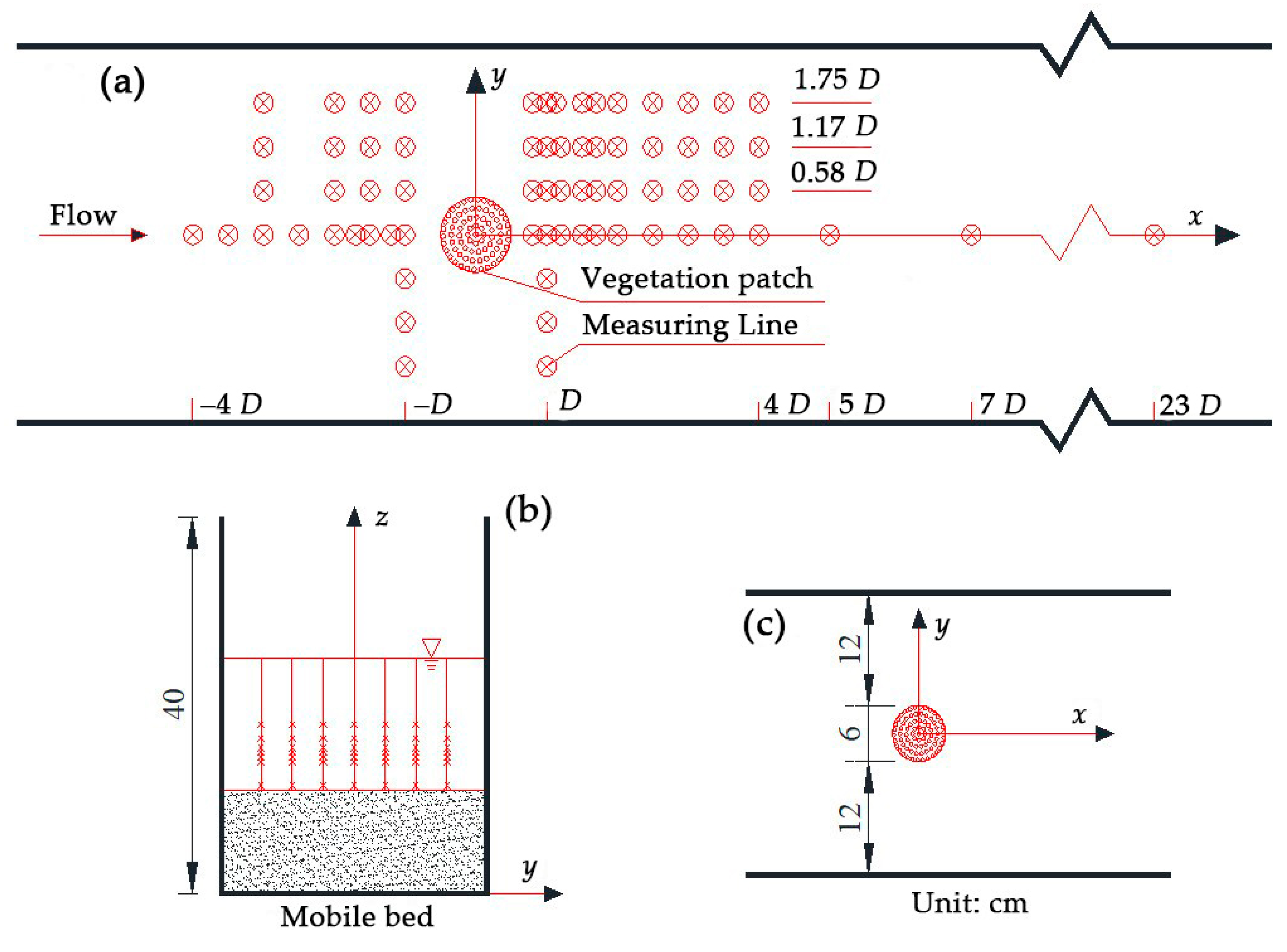
Experiments were conducted in a straight Plexiglas flume with a 16 m long, 0.3 m wide, 0.4 m high, and 1.62 m long test section at the State Key Laboratory of Hydraulics and Mountain River Engineering (SKLH) of Sichuan University, China. A plate gate was arranged at the tag end of the flume, which was used to maintain uniform water flow. Next, a funnel was equipped upstream of the plate gate and a filter screen with a valve at the bottom was connected to collect sediments. We mounted a 3D acoustic Doppler velocimeter (ADV) (Nortek, Bærum, Norway) measuring bracket and a probe system on the sink rail. In addition, fiberglass circular cylinders were used to simulate the rigid and non-submerged vegetation unit. We arranged the vegetation of a single plant into a circular vegetation patch in the staggered pattern, which was then arranged into the punched plexiglass base plate. Table 1 presents all test setup parameters.
The model patch blocked 20% of the channel width, while the patch density (a) was variable. The diameter of each plexiglass circular patch was 6 cm, which was much smaller than the flume width. The cylinder diameter (d) was set to 4 mm. Notably, the diameter of real emergent vegetation stems varied from 1 mm to 10 mm [27,28]. We used the following equation to estimate the vegetation patch density: a = nd, where n and d are the plant number in the unit vegetation area and the diameter of the single plant, respectively. Furthermore, the flow discharge rate and the water depth were set to Q = 18.01 L/s and H = 13 ± 0.2 cm, respectively. Then, the average cross-section velocity, U0, could be evaluated. Figure 1 illustrates the pattern of the vegetation community and the arrangement of the measuring points.
In the case of the mobile bed, the bed was paved with uniform sediments, where the grain diameter, vertical depth, and length were 1.5 mm, 0.11 m, and 10.4 m, respectively, per Chien and Wan [29]. In addition, the length of the upstream gravel transition and the testing sections were set to 1.00 and 1.62 m, respectively. We measured the flume slope by the spirit level with a measurement accuracy of 1%, which was measured and calculated repeatedly. Under this experimental condition, we obtained a clear movement of the bed load, but the results of this study are not valid for the suspended load.
We measured velocities with the ADV along the x-axis upstream and downstream of the patch. The sampling volume of ADV was located from the bottom to the middle of the flow depth. At each point, three velocity components (u, v, and w) were recorded with a sampling rate of 50 Hz for 30 s. Furthermore, H and U0 denote the flow depth and the average velocity in a cross-section; D denote the diameter of patch. In this experiment, repeated trials for each test case were conducted.
There were 7 and 25 measuring sections upstream and downstream of the model patch, respectively, to measure the velocity and position of particles accurately; this was intended to monitor the flow characteristics from −4 D to 23 D of the model patch. As velocity gradients near the model patch were high, the interval between the measuring sections decreased near the vegetation community. Each section had seven vertical measuring lines, where the lateral values of the y-coordinates from the far left to the far right were 1.75 D, 1.17 D, 0.58 D, 0 D, −0.58 D, −1.17 D, and −1.75 D. In addition, there were eight testing points, which were evenly distributed along the width and depth. For vertical distances from the measuring point to the bed that were <5 mm, the measuring interval was set to 1 mm, while for distances >5 mm, measuring intervals were set to 5 mm and 10 mm, in accordance with the particular flow depth.
The turbulent kinetic energy depicts the balance between the increased turbulence intensity because of wake effects of canes and the decreased flow rate through the canopy [15,30]. The turbulent kinetic energy is defined as follows:
where TKE is the turbulent kinetic energy and u’, v’, and w’ are the flow velocity fluctuations in the x, y, and z directions, respectively.
Each velocity record was decomposed into its time-averaged (, ) and fluctuating components (, ). The over bar depicts the time-averaging operator. We estimated turbulence fluctuation intensities as the root-mean-square of the fluctuating velocities [5]:
After measuring the velocities, we acquired the topographic data using the Nikon Total Station Instrument (Toyoma City, Toyoma, Japan) and the data was processed using the Kriging method.
3. Results and Discussion
3.1. Longitudinal Distribution of the Turbulent Kinetic Energy with Different Vegetation Density
The flow in the channel with the vegetation was a completely developed turbulent flow. The presence of the open-channel vegetation not only affected the average velocity field but also altered the turbulence field. We used the turbulent kinetic energy to illustrate correlations between velocities and wakes.
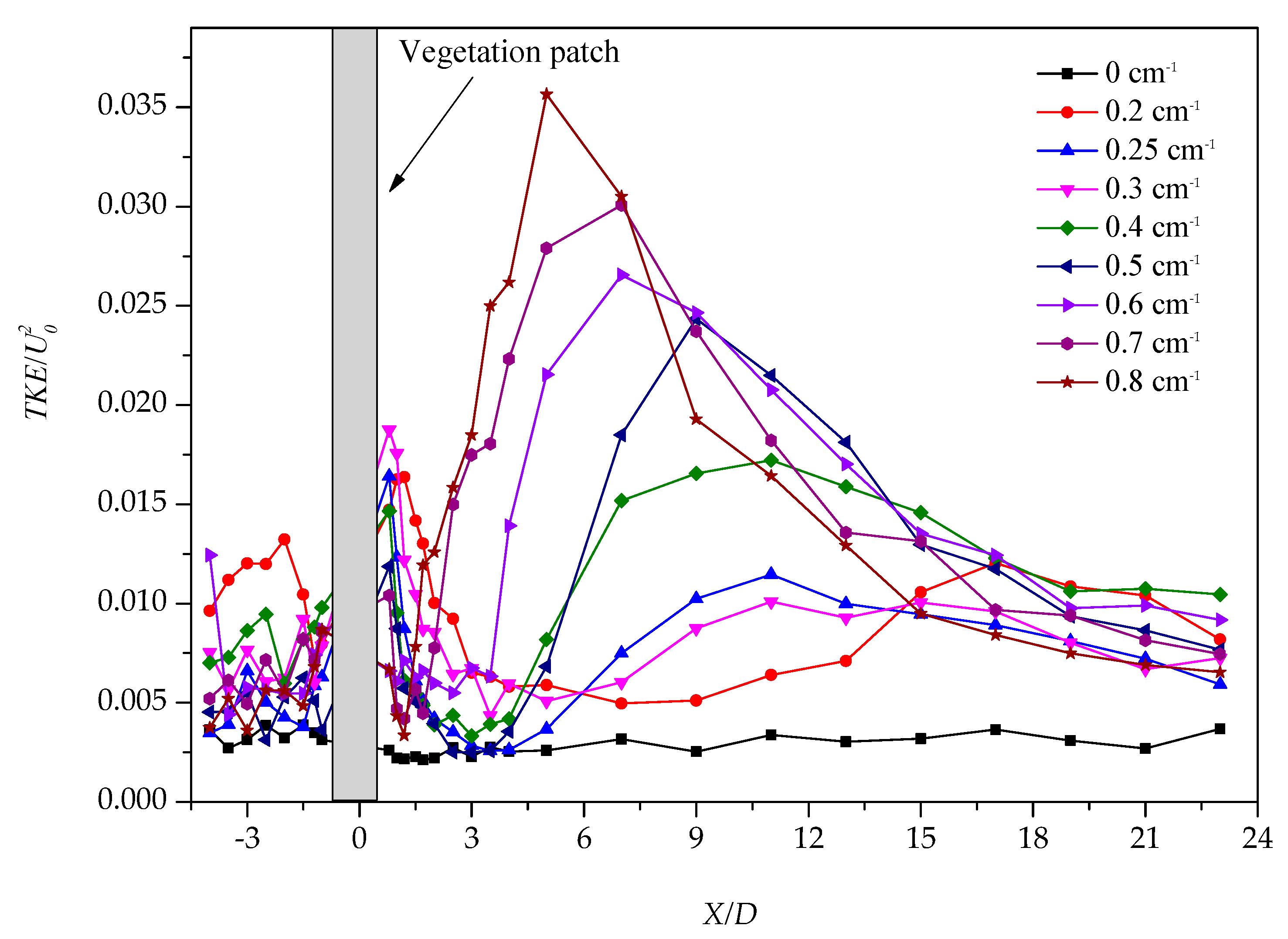
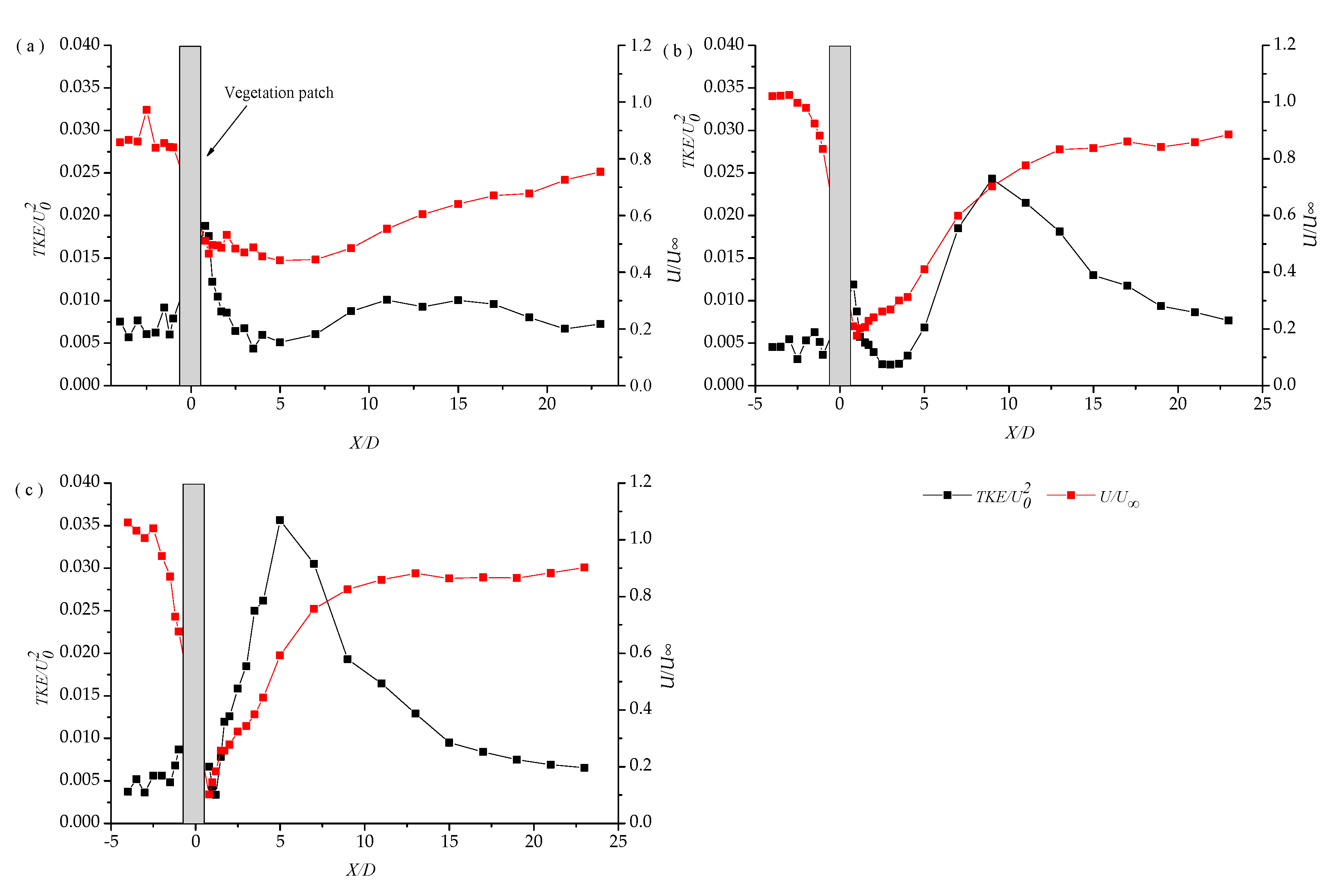
The TKE takes the measuring point at the center line of the rectangle flume at a depth of 0.5 times the water flow; U0 is the average flow velocity, which is measured at a half depth of the upstream section (X/D = −4). Figure 2 presents the longitudinal distribution of dimensionless turbulent energy along the path.
The value of the normalized TKE upstream of the vegetation group did not exhibit an apparent decrease or increase along the X/D axis, suggesting upstream of the patch was less affected by the flow. Conversely, the turbulent kinetic energy of the vegetation group in the downstream varied markedly along the path. Figure 2 suggests that all TKE distributions have two peaks and one trough and finally go stable.
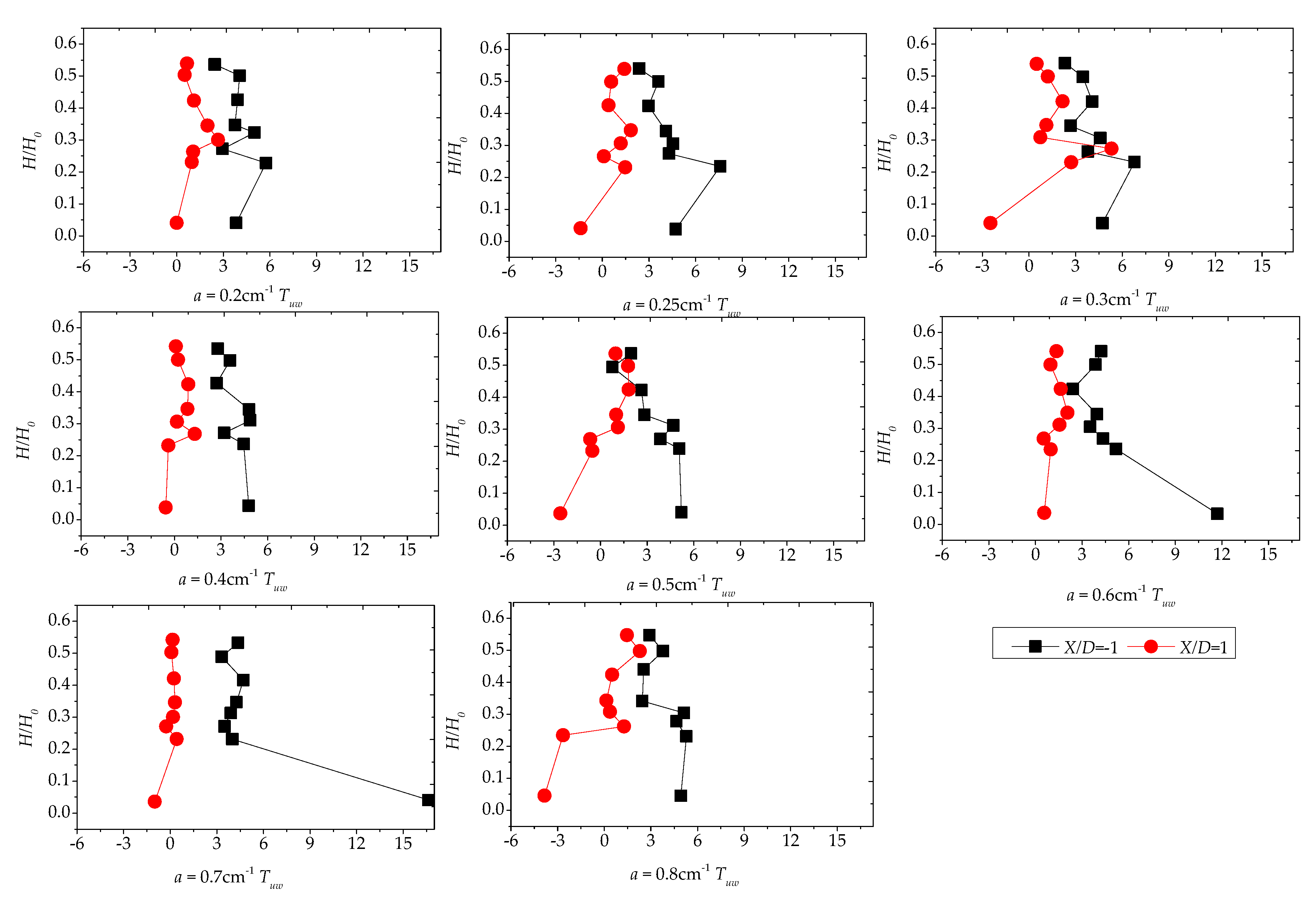
Owing to the impact of different vegetation densities, the first peak simultaneously appeared at 0.8 D. We observed that the height of the peak increased as the vegetation density increased, suggesting that the denser patch could cause a stronger disturbance. The first peak occurred behind the patch. The position that the peak occurred correlated with turbulence production within the patch at the scale of individual cylinders. Actually, the turbulence intensity generated by individual stem wakes was set by the stem-scale Reynolds number, Red = up × d/, and a function of the flow blockage. Notably, up and denote the average velocity within the patch and the kinematic viscosity coefficient, respectively. Furthermore, as Red increases, the peak also increases [13].
However, the turbulence effect of the vegetation was short and the turbulent kinetic energy decreased rapidly, presenting the plant patch with a relatively sparse layout to those dense patches; for example, the density of vegetation is a = 0.8 cm−1 and the range between the first peak and trough was longer. Here, the range is the steady wake region, which is the distance between the patch and the formation point of the vortex street [5]. In addition, the rebounding momentum from the line bottom correlated with the denseness and there existed a minimum turbulence level between the two peaks which was lower than the turbulence level of the undisturbed upstream flow [13].
Nevertheless, different shear layers were established because of the interaction between two different flow rates in the wake region of the vegetation. As the width of the shear layer continued to increase along the longitudinal direction, it met at a certain point to form the Von Karman vortex street. The produced turbulent vortex by the Von Karman vortex street maximized the turbulence of the water flow. Thus, the second turbulent energy peak appeared. Then, the turbulent energy began to weaken and finally stabilized. When the vegetation became sparse (a = 0–0.3 cm−1), the subsequent peak appeared near 15 D. As the density changed, the position of the second peak increased gradually and the peak increased. The analysis presented above demonstrates that the higher the vegetation density, the earlier the appearance position of the Von Karman vortex street and the greater the turbulence peak caused by the Von Karman vortex street, suggesting that the strength of the Von Karman vortex street was increasing.
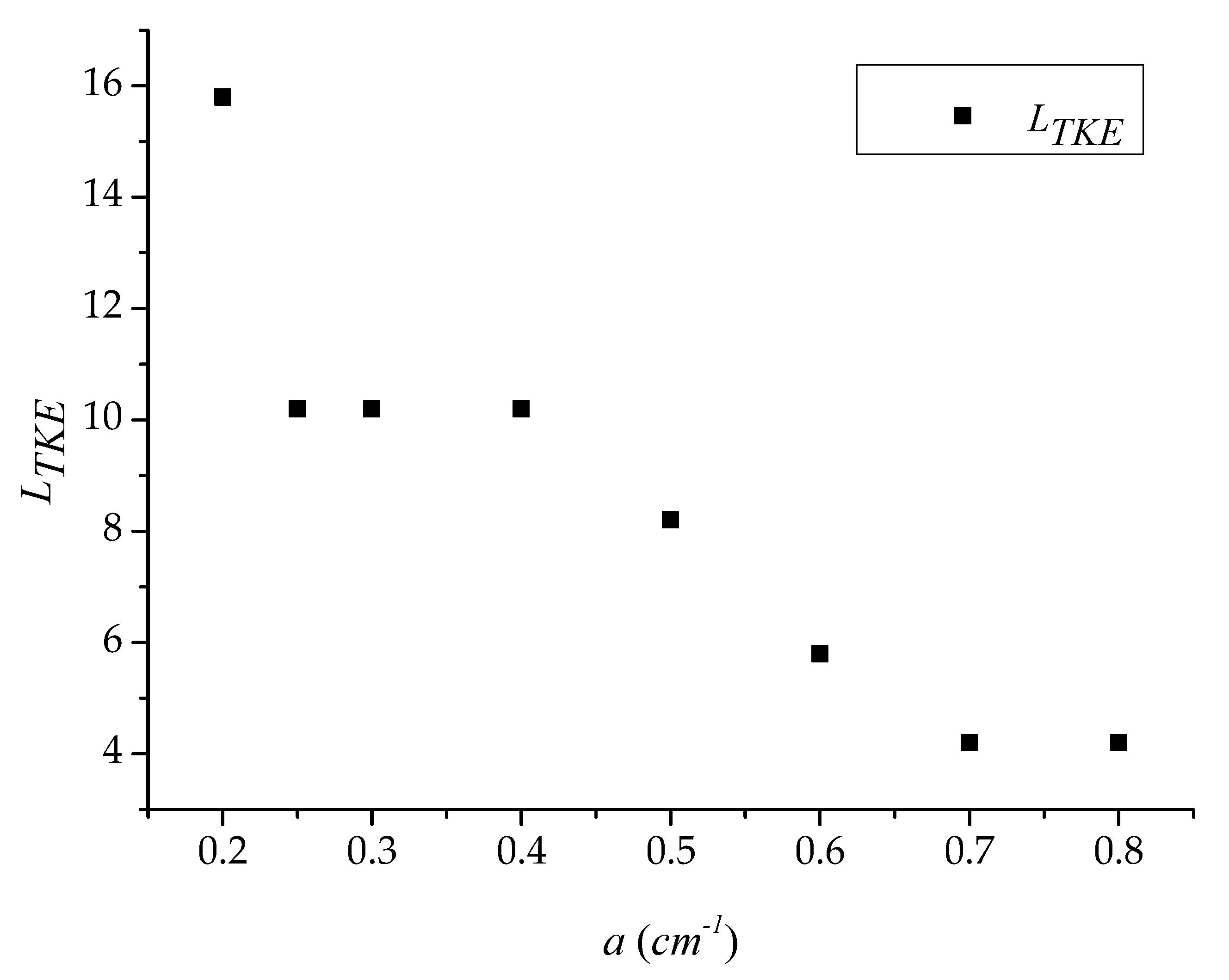
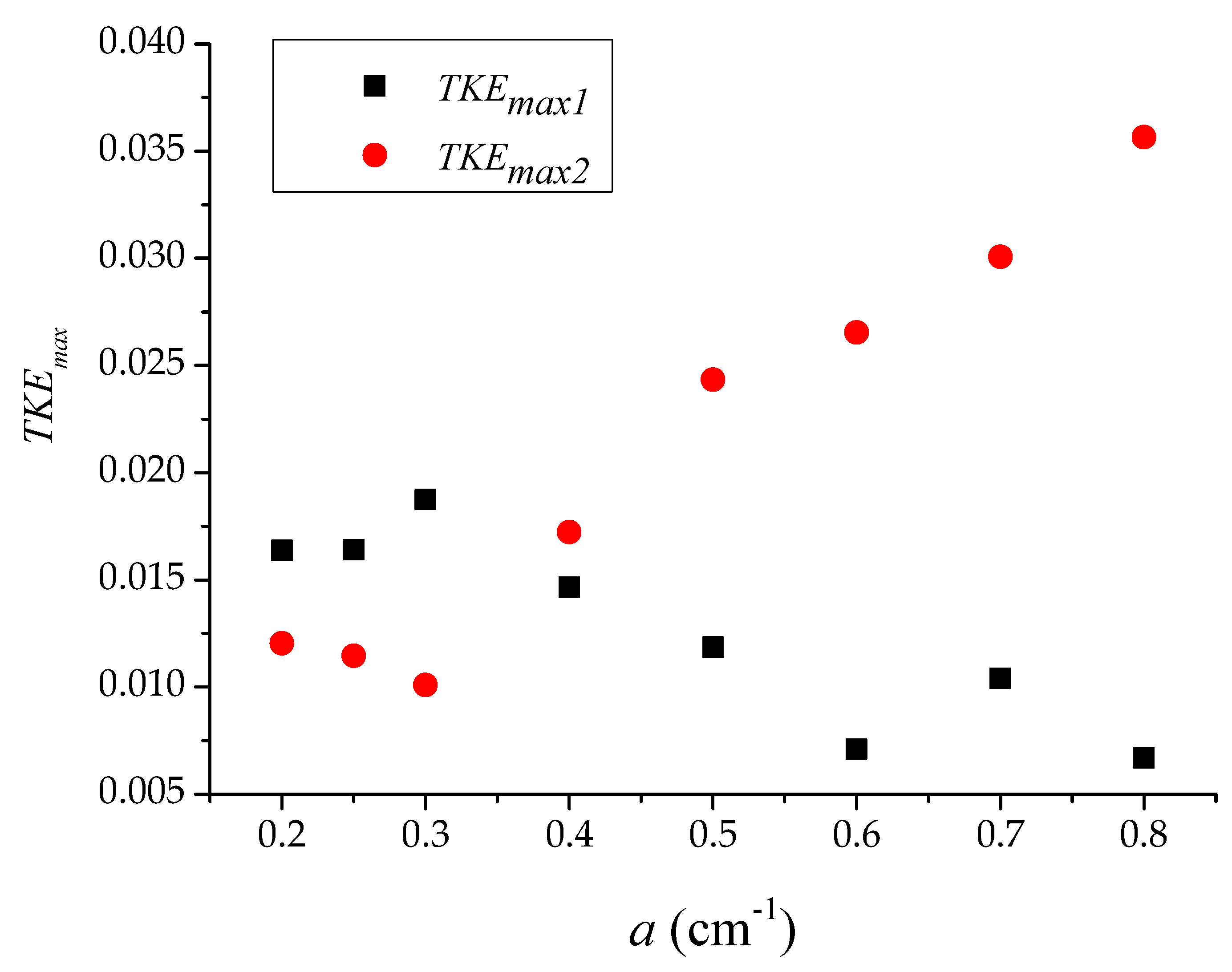
The distance between two turbulent energy peaks (TKEmax1 and TKEmax2) was defined as LTKE. We analyzed the correlation between LTKE and the vegetation group density, a. Figure 3 shows that the density, a, of the vegetation group increased, but LTKE gradually decreased. When a = 0.5 cm−1, the length of the LTKE tended to be stable. In addition, the position of the peak was basically stable at x = 9 D, suggesting the formation of the Von Karman vortex. The position of the street initially moved forward with the increase of the density of the vegetation group. When a reached a certain level, the position of the Von Karman vortex street was no longer affected by a. Figure 3 and Figure 4 show that the position where the valley TKEmax1 appears coincides with the positional trend of the peak TKEmax2. In particular, it gradually moved forward and finally became stable. Furthermore, Figure 4 shows that the speed at which TKEmax2 advanced was faster than TKEmax1; thus, the slope between the valley and the second peak TKEmax2 becomes increasingly steeper. Moreover, when the vortex street was delayed downstream, it also degraded more slowly.
Discussing rigid and emergent aquatic vegetation as a porous obstruction in some way is a comprehensible approach. Figure 2 shows that the double peak in the turbulence intensity exists in other porous obstructions. In addition, Figure 3 shows that the density of patch and the strength of the bleed flow correlate positively, resulting in the creation of the Von Karman vortex street far downstream of the wake [5,31]. The obstruction with a high fence porosity ɛ is like a sparser vegetation patch. Lee and Kim [32] reported that the intensity of the second turbulence peak decreased as the fence porosity increased; likewise, Castro [12] reported a similar observation behind thin perforated plates.
Figure 4 further presents the correlation between two relative turbulent energy peaks (TKEmax1 and TKEmax2) and the vegetation group density a. The first turbulent peak (TKEmax1) after the vegetation group was distributed in a wave manner with the increase in the density, a, of the vegetation group. Figure 4 suggests that the fluctuation range of TKEmax1 was short, whereas the second turbulent peak (TKEmax2) presented a large fluctuation range. Furthermore, TKEmax1 increased as the density a increased. The growth rate of TKEmax2 decreased first and then increased. When a = 0.8 cm−1, the turbulent kinetic energy reached its peak value.
Furthermore, a comparison of two trend lines revealed that the value of TKEmax1 was higher than that of TKEmax2 in the low-density vegetation group and the turbulence intensity after the vegetation group predominated. As the density of vegetation groups increased, the role of the Von Karman vortex street became pivotal, which led to a rapid increase in the peak value TKEmax2. Figure 4 suggests that when a ≈ 0.38 cm−1, two values of TKE were equal. With the denser vegetation, the turbulence effect generated by the Von Karman vortex street took the main advantage, making the value of TKEmax2 much higher than that of TKEmax1.
As TKEmax2 and TKEmax1 had opposing tendencies with increasing density (Figure 4), the following transition occurred. For low densities (a ≤ 0.3 cm−1), the turbulence reached the highest value immediately downstream of the patch; however, for a denser patch, the turbulence intensity was highest at some distance far from the patch [13,33].
3.2. Lateral Distribution of Stream-Wise TKE with Different Vegetation Densities
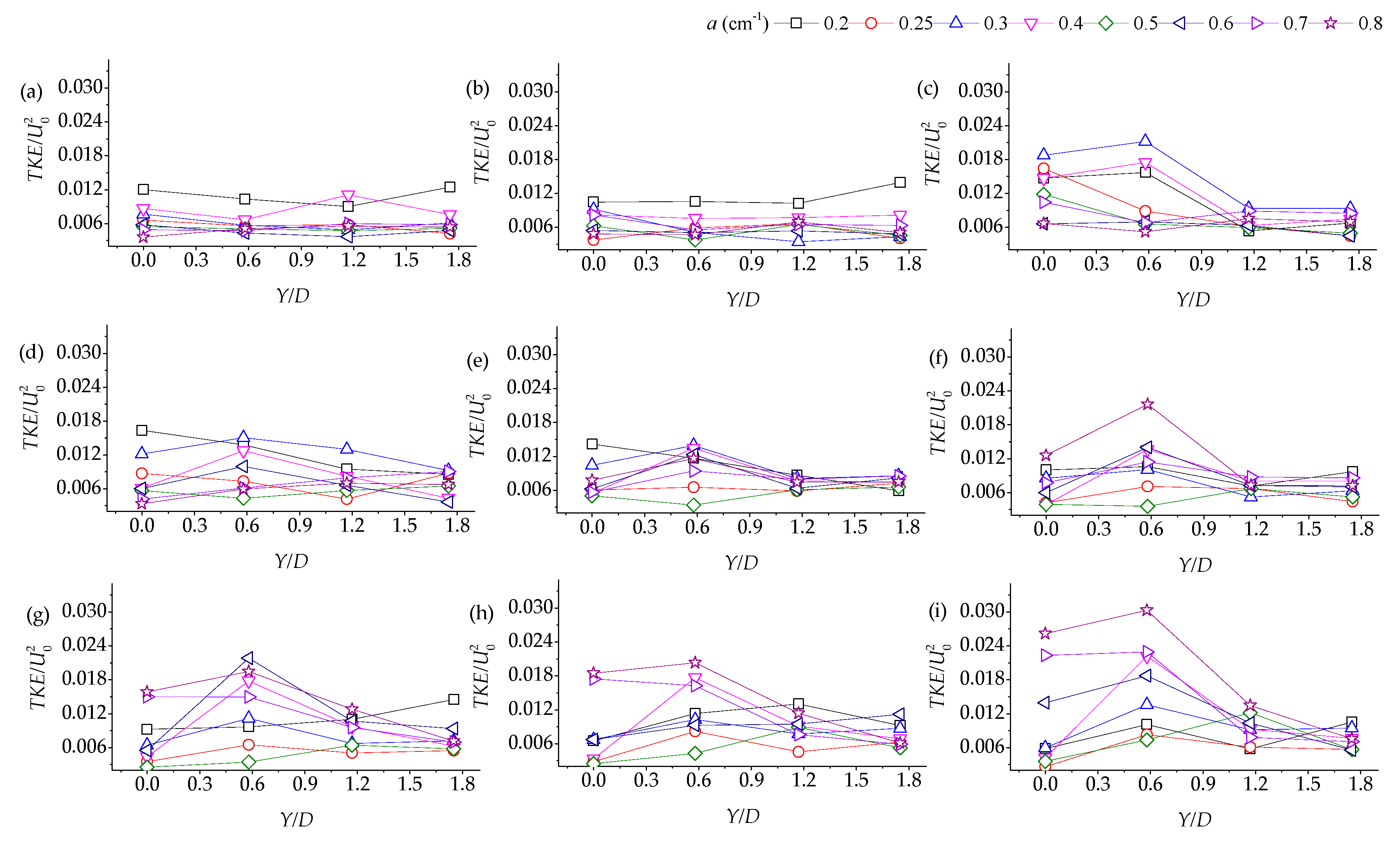
We obtained the turbulent kinetic energy of the water flow at a half-water depth of X/D = ±1. As the channel and the vegetation layout were symmetrical, only half of it is presented. Figure 5 illustrates the lateral turbulent energy distribution.
When upstream flows were provided, the vegetation group density exhibited no impact on the lateral distribution of the TKE of the patch front edge, so the performance along the path was a straight line. Downstream of the vegetation group, the transverse distribution of the turbulent kinetic energy exhibited a similar shape at different densities of the patches. The maximum value of TKE occurred at the left and right ends of the vegetation patch (a > 0.3 cm−1). We observed a positive correlation between the maximum turbulent kinetic energy of the patch and the density. Compared with the brink of the patch, the turbulent kinetic energy was marginally smaller at the centerline behind the patch. Furthermore, beyond the range from centerline to Y/D = 1.2, the value of TKE was stable. As the measured section became farther away from the patch, the difference in TKE between low and high density patches increased.
When the water flowed through the vegetation group, the water flow was partially separated; as the flow velocity on both sides of the vegetation group increased, the turbulent kinetic energy also increased and as the flow velocity at the centerline was relatively small, the turbulent kinetic energy decreased accordingly. Some studies focused on the transverse velocity fluctuation (), which is at its maximum at the wake center. The magnitude of decreased monotonically toward the edge of the wake, which is characteristic of a vortex street [5,34,35].
3.3. Vertical Distribution of the Turbulent Intensity with Altered Plant Patch Density
Next, we considered the vertical structure of the turbulence intensity and its evolution downstream. Thus, we analyzed the measured data in a certain area upstream and downstream of the vegetation group. Locations at the centerline of the section (X/D = ±1, Y/D = 0) were selected to investigate the vertical variation of the turbulence intensity near the vegetation area with different densities. Figure 6 shows the vertical distribution of the turbulent energy at a distinct vegetation patch at X/D = ±1.
Figure 6a shows that the upstream of a vegetation group is less affected by the flora and the turbulence intensity under different vegetation density exhibits a similar trend with the water depth; that is, the water depth first increased but then decreased. However, in some cases, the high density of plants affected the change of upstream turbulence. When a group of plant’s densities measured a = 0.6, 0.7, and 0.8 cm−1, their dense structure led to backwater, which affected the turbulent energy in the range of H/H0 = 0.2–0.3; the turbulent energy decreased. Hence, for plants with relatively high densities, the law of change describes an initial increase, then a decrease, and then a rise as the water depth increases.
Figure 6b suggests that, at the extremity of the vegetation group, the distribution of turbulent energy with the water depth was relatively similar to upstream of the vegetation patch, which could be attributed to the impact of altered density vegetation on the flow. However, the bottom turbulence value marginally decreased compared with that for upstream of the vegetation patch with a relative water depth of 0.04; this is attributed to the creation of small eddy current after the vegetation group so that the flow disturbance increased, but the flow velocity decreased rapidly. Thus, the turbulence intensity increased after the vegetation group; however, the increase in the flow rate was not notable. Furthermore, plant density and water depth increased, the turbulent energy decreased, and the variation range became smaller. Figure 6 presents a more stable S-shaped distribution.
Typically, the vertical distributions of the turbulence intensity tended to be “S” type and there were turning points at H/H0 = 0.25. In the wake region, the peak of occurred far from the channel bed and irregular variation of the peak value of was attributed to detached eddies from upstream cylinders [36].
In this study, the turbulent energy at the upstream of the vegetation group did not exhibit a clear correlation with the density, but it did exhibit a positive linear correlation with the vegetation density downstream of the vegetation.
We added turbulence distributions for a = 0 to Figure 6a,b to further explain this phenomenon. The density of the vegetation group exerted a significant impact on the vertical distribution of the turbulent energy of the water flow. When the vegetation groups were sparse, the turbulent energy fluctuated markedly, along with the water depth. The extreme situation occurred for a = 0, where the vertical distribution curve had two inflection points and the vertical distribution of the turbulent energy was in a zigzag shape. Of note, the number of inflection points decreased to one point and eventually disappeared. Figure 6 shows that the vertical distribution of the turbulent energy is close to a vertical line.
Figure 6 and Figure 7 show that the density of the vegetation group is a vital factor affecting the vertical distribution of turbulent energy. When the density of vegetation groups increased, interactions between the water flow and the vegetation group increased. In addition, the energy carried by the water flow was evident in the case of constant upstream flow. When the water flowed through the vegetation group, the energy carried by the unit volume water flow decreased, the turbulent energy of the water flow reduced, and the variation of the water depth reduced; this was presented in the vertical direction of the turbulent energy distribution. Furthermore, the distribution pattern gradually developed from a fold line into a vertical line and the breakpoint on the vertical distribution gradually disappeared as the density of the vegetation group increased.
With the increase of the vegetation group density, the vertical distribution of the turbulence intensity changed more severely. The starting position of this trend gradually neared the vegetation group. Furthermore, the median value of the vertical distribution along each section increased.
The analysis presented shows that, when river channels and the upstream flow reach a certain value, the vegetation community exerts a remarkable impact on the vertical distribution development of the turbulent kinetic energy of the downstream river channel. In the vertical distribution, the density variation is the most effective parameter. We noted that when the patch was sparse, the flow through plants and the recirculating flow affected the position and the inflection point of the vertical turbulence appeared. On the other hand, for the dense vegetation, the gaps between plants were tight. As the impact of the bleed flow decreased, vortex streets were formed closer to each other so that the turbulence intensity of the vegetation patch changed greatly.
3.4. Reynolds Stress Distribution of Different Vegetation Density
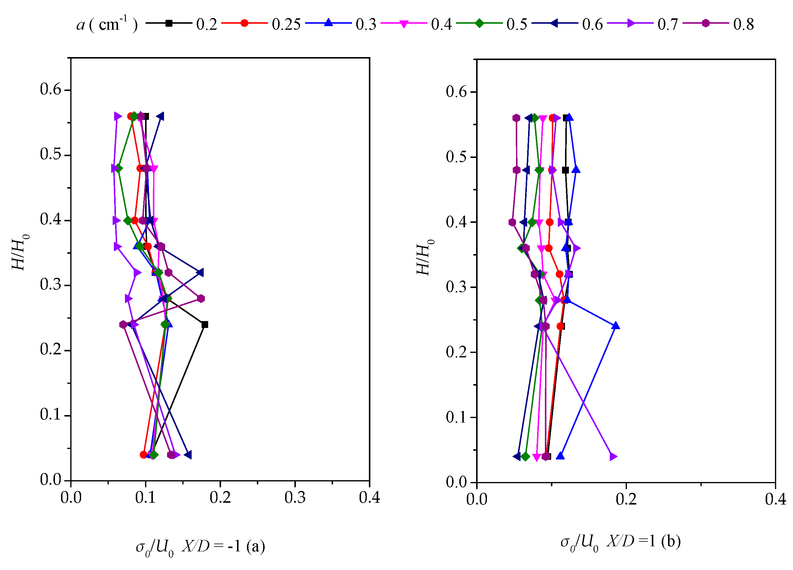
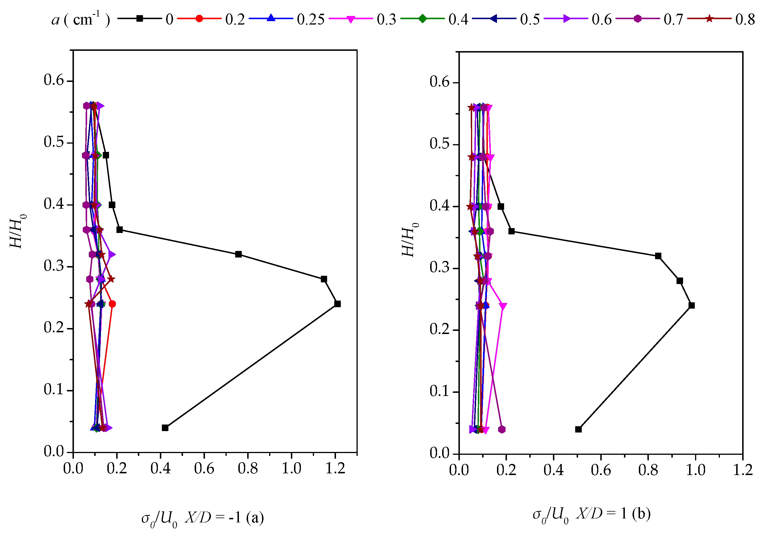
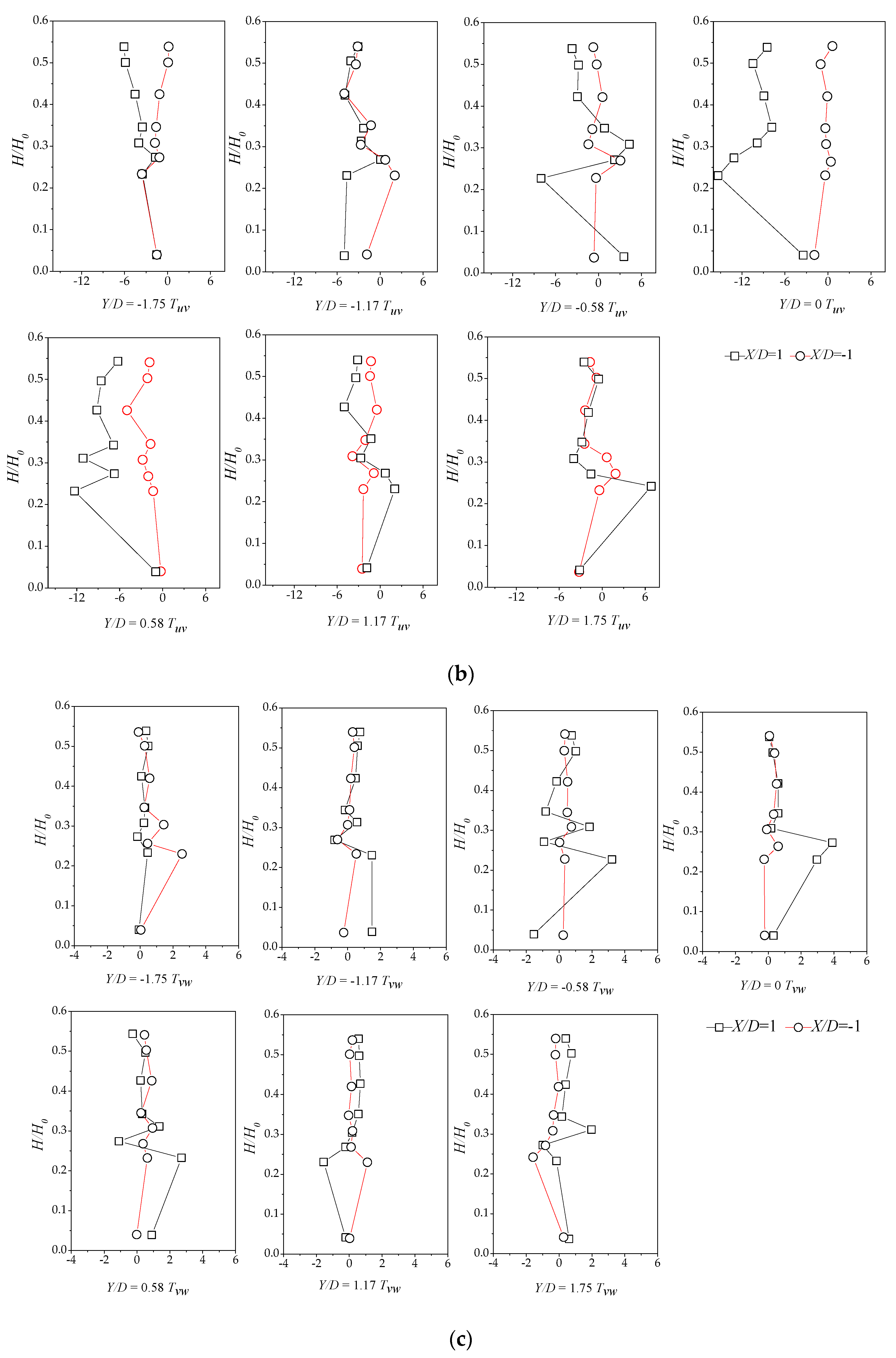
Here, we discuss Reynolds stress distributions of different plant group densities. The Reynolds stress was generated because of uneven distributions of the flow velocity in the flow field. The greater the Reynolds stress, the more uneven the flow velocity distribution and the more turbulence intensity was present. As the Reynolds stress directly correlates with the exerted water force on the bed, it is a useful predictor of areas of sedimentation and erosion [15]. Figure 8a–c and Figure 9 show the vertical distribution of the Reynolds shear stress on the cross-section at X/D = −1 and X/D = 1 for the vegetation patch with a density of a = 0.3 cm−1. Figure 8a shows the Reynolds shear stress, defined as . Figure 8a indicates that the Reynold shear stress exhibits significant fluctuations. The sign of the shear stress suggests the direction of the momentum flux. In a Cartesian coordinate system, negative values depict momentum flux toward the bed [15]. We observed a maximum in the shear stress distribution of H/H0 = 0.25. The difference in the Reynolds shear stresses increased gradually at X/D = −1 and X/D = 1 from line Y/D = −1.17 to Y/D = 0.58. The difference reached the maximum value on the centerline, behind the plant group. Furthermore, the difference gradually declined toward the left bank. Perhaps, the scatter in the profile of Y/D = ±0.58 is attributable to irregular detachment of wake vortices.
Figure 8b depicts the vertical distribution of the shear stress, defined by . The value of the Reynolds shear stress at the centerline and downstream at X/D = 1 is much smaller than that of the downstream (X/D = −1). The prevalence of outward and inward events is accountable for the decreasing magnitude of the shear stress at X/D = 1. In addition, the difference in the vertical distribution on both sides of the centerline becomes smaller as it gets closer to the sidewall. A comparison of Figure 8a,b reveals that the vertical distribution of two Reynolds shear stresses fluctuates markedly for H/H0, varying from 0.2 to 0.3, which could be the most intense place for the bleed flow and the recirculated flow, suggesting that the bed influence on the vertical distribution of the Reynolds stress is limited.
Figure 8c illustrates the vertical distribution of the shear stress, defined by , with a relative water depth of 0.3 as the boundary. In the upper part (H/H0 > 0.3), the distribution of the shear stress at the upper and lower parts of the cross-section is comparable and the shear stress is uniformly distributed. At the range of H/H0 = 0–0.3, starting from the line adjacent to the right bank of the water tank, the upstream shear stress is higher than the one from the downstream. Meanwhile, as it approaches the centerline, the downstream shear stress slowly increases because of the impact of the plant group and attains the maximum value of Y/D = 0.
Sedimentation and erosion processes are profiles of the vertical momentum flux () [15]. Figure 9 shows the vegetation density effect on the Reynolds shear stress, where Tuw is related to the water depth change at X/D = ±1 and Y/D = 0, demonstrating that u0w0 is positive at X/D = 1. Hence, momentum transport is upward into the water column. Furthermore, we found extremum Reynolds stress values behind the patch with low densities (a < 0.3 cm−1) at H/H0 = 0.25, while the highest values of u0w0 always took place near the bed.
Combined with the lateral turbulence distribution, the high density makes the plant group flow around and the gap flow weakens, explaining why the shear stress near the bed surface of the downstream centerline varies with the density variation. For boundaries with H/H0 = 0.25, the difference between the upper and lower shear stresses of above and below the boundary line is small; this difference below the boundary line becomes larger as the water depth increases or decreases. From another perspective, the denser group offers the vegetation group more control over the back-shear stress, also implying that the dense vegetation group exerts more impact on the upstream flow.
Based on the analysis presented above, the dense plant structure could affect the distribution of the turbulence and shear stress, shorten the intersection distance between two shear planes from the vegetation, and increase the length of the freely developed turbulence zone. Meanwhile, dense plants affect the shape of the bed surface and form a symmetrical scouring area on both sides of the centerline. Thus, the denser a plant, the higher the stacking height and the clearer the scouring area.
4. Impact of Turbulence with Altered Vegetation Densities on the Sedimentation
Prior experiments have focused on the biogeomorphic evolution. Through numerical modeling, Lopez and Garcia [19] highlighted that the suspended sediment transport is decreased in vegetated streams because of the reduced bed shear stress; this is used as a proxy to compare the sedimentation and erosion patterns of the flowfield. A straightforward correlation exists between the TKE () and the bed shear stress , , where c1 and are real constants (c1 ≈ 0.2) and the water density respectively [37]. Although it is not an accurate method to derive absolute values of from the ADV data, a strong correlation exists between the near-bed turbulence and bed shear stress. In addition, research has highlighted that the turbulence might dislodge individual sediment particles and could affect the net deposition [38,39,40,41,42]. Hence, a study was proposed to compare spatial patterns of the near-bed Reynolds stress and the turbulence intensity in the model [15].
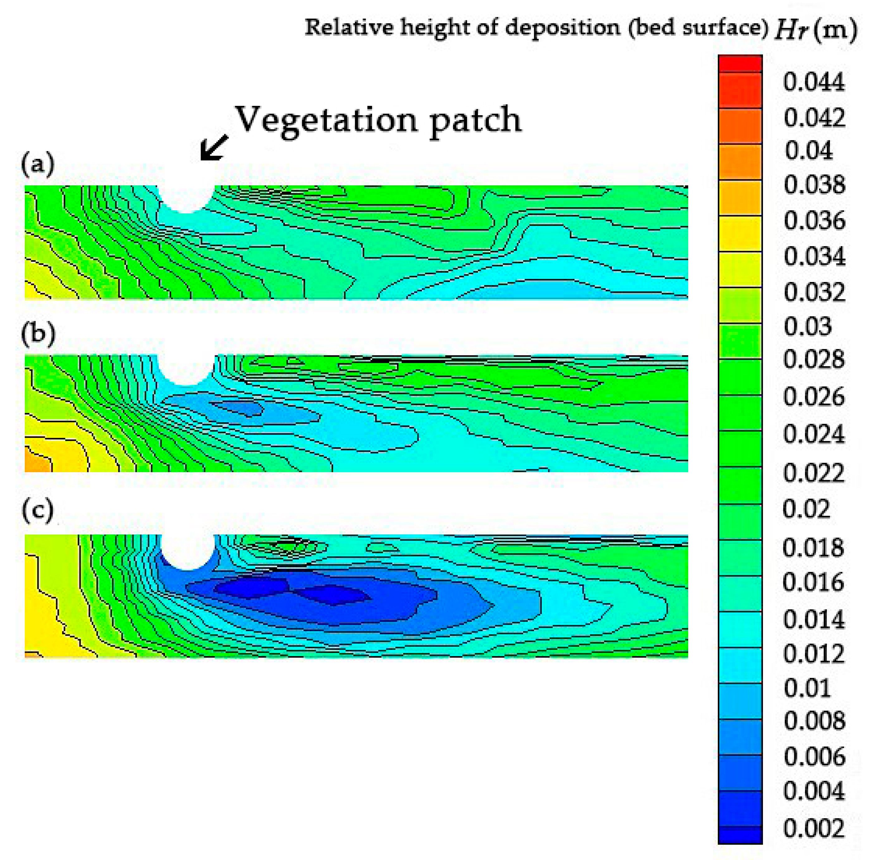
Reportedly, enhanced deposition upstream was observed in a vegetated region [21,43], which could be attributed to the deceleration of the flow, bed shear stress (Figure 10), and high levels of erosion at the leading edge of high-density patches (Figure 11). Although we did not measure the deposition inside the dense patch in this study, previous studies reported the elevated TKE and scouring within dense patches [44].
Meanwhile, the deposition of fine sediments was reported in the wake behind a patch [13], which, along with the diminished deposition near the leading edge, could illustrate why patches grow in length predominantly in the downstream direction [45].
Figure 2 and Figure 10 suggest a near wake region downstream the patch where both velocity and TKE are diminished so that the deposition of fine particles increases. In fact, the variation of the turbulent kinetic energy closely correlates with the variation of the velocity. The decrease in the velocity and turbulent kinetic energy is attributed to the sedimentation after plant. Figure 10 suggests that the increase in density exerts a significant impact on the reduction of velocity and turbulent kinetic energy; this change results in a shorter length of the sedimentary area but a larger maximum height of the sedimentary area. The flow rate gradually recovers far from plants and, meanwhile, the turbulent kinetic energy decreases and the bed surface scours.
The low density of patches occurs frequently. Strong bleed flow protects sediments from erosion, by extending the boundary layer to prolong the outset of the vortex street and displace the high Reynolds stresses to an area higher up in the water column; thus, they tend to get a much longer LTKE than a high-density patch. However, increasing turbulence and associated elevated vertical diffusivity might enhance resuspension and facilitate sediment transport. Furthermore, the deposition is depressed beyond this region because of the enhanced TKE associated with the Von Karman vortex street [13,19,30]; however, it can dominate the situation through the vortex street.
The sparse patch generates a much longer region of enhanced deposition; however, it does not span the patch width so that the lateral deflection of the flow around a finite patch can increase the velocity along the patch edge [8,15,46,47]. In addition, enhanced erosion occurs only in regions where both turbulent and mean velocities increase, compared with those in the open channel. Considering the “M” shape of the lateral distribution of the dimensionless TKE (Figure 5), it is inferred that two regions of bed erosion and restricted lateral growth of the patch resulted in negative feedback for the lateral patch expansion.
In fact, variations of the bed topography also affect the turbulent energy patterns. Upstream of the dense patch, we observed high shear stress. The water flow produces shear stress on the bed surface and the bed generates a reaction force against the water flow, called resistance. The increase of the plant population density and resistance decreases the water flow velocity (Figure 10). In addition, the bed surface is continuously scoured by the flow and the turbulent kinetic energy grows slowly. In the centerline downstream of the plant population, the change in sedimentation depicts the change in the turbulent kinetic energy. Furthermore, the sedimentation peak maximizes the turbulent kinetic energy. Due to a lack of resistance from the plant and the bed to the current, the flow rate gradually returns to the upstream value.
This study proposes that positive feedback is stronger for sparse emergent patches, which create longer regions of the enhanced deposition. Patch configurations lead to a relatively quiescent region, immediately downstream of the plant patch. This is a region where plants can grow easier. Alternatively, the erosion resistance of the riverbank with luxuriant growth of emerged plants has been enhanced, which ascertains the capacity of the boundary to constrain the hydrodynamic axis migration [48,49]; this is an example of ecosystem engineering, where organisms alter their physical habitat to obtain an advantage over other organisms [50]. Investigating the impact of plant density on the wake structure for moving beds could elucidate vegetation flow into dense, sparse, and isolated flow, based on threshold parameters [36]. Furthermore, mathematical modeling of turbulence hydrodynamics in an emergent vegetated open-channel flow could be verified with the presented experimental data.
5. Conclusions
To date, various experiments have shown that the vegetation of different densities exerts a profound impact on the distribution of the post-turbulent kinetic energy. By demonstrating its inherent laws, it also provides a basis for investigating the fluvial process, sandbank formation, and digital model establishment.
The longitudinal distribution of turbulent energy correlates with the density, generating two peaks—stem-generated wake peak and maximum wake recirculation. The distance between the peaks negatively correlates with the density, whereas the peak height positively correlates with it; this alters the region of the enhanced deposition. In addition, this correlation could provide ecologists with a framework to comprehend the reaction among vegetation, flow, deposition, and growth. The lateral distribution suddenly decreases in turbulent kinetic energy at the centerline. The patch density and the distance from the origin are positive factors that maximize later distribution.
This study establishes that for the vertical distribution of the shear stress from a certain section, as the density decreases, the tendency to be a straight line increases. In addition, with H/H0 = 0.25 as the boundary, as the shear stress nears the bed surface, the turbulence intensity increases. This study shows that dense patched exert a significant impact on the rear turbulence. Meanwhile, distributions of the Reynolds shears stress are considered for further study of various density vegetation patches. The rear deposition is symmetrically distributed along the centerline, similar to the turbulent energy distribution of the transverse section. Finally, this study deduces that a dense plant group could weaken shear forces from the upstream.
Author Contributions
Conceptualization, Z.Y.; investigation, Z.Y.; methodology, Z.Y. visualization, Z.Y.; writing—original draft, Z.Y.; writing—review and editing, Z.Y. and D.W.; supervision, X.L.
Funding
This research work is supported by the National Key Research and Development Program of China (No.2016YFC0402302) and the National Natural Science Foundation of China (No. 51609160).
Acknowledgments
Many thanks to the State Key Laboratory of Hydraulics and Mountain River Engineering, Sichuan University.
Conflicts of Interest
The authors declare no conflict of interest. The founding sponsors had no role in the design of the study; in the collection, analyses, or interpretation of data; in the writing of the manuscript, and in the decision to publish the results.
References
- Chen, S.; Chan, H.; Li, Y. Observations on flow and local scour around submerged flexible vegetation. Adv. Water Resour. 2012, 43, 28–37. [Google Scholar] [CrossRef]
- Corenblit, D.; Tabacchi, E.; Steiger, J.; Gurnell, A.M. Reciprocal interactions and adjustments between fluvial landforms and vegetation dynamics in river corridors: A review of complementary approaches. Earth-Sci. Rev. 2007, 84, 56–86. [Google Scholar] [CrossRef]
- Vandenbruwaene, W.; Temmerman, S.; Bouma, T.J.; Klaassen, P.C.; De Vries, M.B.; Callaghan, D.P.; van Steeg, P.; Dekker, F.; van Duren, L.A.; Martini, E.; et al. Flow interaction with dynamic vegetation patches: Implications for bio-geomorphic evolution of a tidal land-scape. J. Geophys. Res. 2011, 116, F01008. [Google Scholar] [CrossRef]
- Bouma, T.J.; De Vries, M.B.; Low, E.; Peralta, G.; Tanczos, I.C.; Van De Koppel, J.; Herman, P.M.J. Trade-offs related to ecosystem engineering: A case study on stiffness of emerging macrophytes. Ecology 2005, 86, 2187–2199. [Google Scholar] [CrossRef]
- Zong, L.; Nepf, H. Vortex development behind a finite porous obstruction in a channel. J. Fluid Mech. 2011, 691, 368–391. [Google Scholar] [CrossRef]
- Zhang, H.; Wang, Z.; Dai, L.; Xu, W. Influence of vegetation on turbulence characteristics and Reynolds shear stress in partly vegetated channel. J. Fluids Eng. 2015, 137, 061201. [Google Scholar] [CrossRef]
- Nezu, I.; Onitsuka, K. Turbulent structures in partly vegetated open-channel flows with LDA and PIV measurements. J. Hydraul. Res. 2001, 39, 629–642. [Google Scholar] [CrossRef]
- Balke, T.; Klaassen, P.C.; Garbutt, A.; van der Wal, D.; Herman, P.M.J.; Bouma, T.J. Conditional outcome of ecosystem engineering: A case study on tussocks of the salt marsh pioneer Spartina anglica. Geomorphology 2012, 153, 232–238. [Google Scholar] [CrossRef]
- Ortiz, A.C.; Ashton, A.; Nepf, H.M. Mean and turbulent velocity fields near rigid and flexible plants and the implications for deposition. J. Geophys. Res. Earth Surf. 2013, 118, 2585–2599. [Google Scholar] [CrossRef]
- Chang, K.; Constantinescu, G. Numerical investigation of flow and turbulence structure through and around a circular array of rigid cylinders. J. Fluid Mech. 2015, 776, 161–199. [Google Scholar] [CrossRef]
- Hu, Z.H.; Lei, J.R.; Liu, C.; Nepf, H. Wake structure and sediment deposition behind models of submerged vegetation with and without flexible leaves. Adv. Water Resour. 2018, 118, 28–38. [Google Scholar] [CrossRef] [Green Version]
- Castro, I.P. Wake characteristics of two-dimensional perforated plates normal to an air-stream. J. Fluid Mech. 1971, 46, 599–609. [Google Scholar] [CrossRef]
- Chen, Z.; Ortiz, A.; Zong, L.J.; Nepf, H. The wake structure downstream of a porous obstruction with implications for deposition near a finite patch of emergent vegetation. Water Resour. Res. 2012, 48, W09517. [Google Scholar] [CrossRef]
- Liu, C.; Nepf, H. Sediment deposition within and around a finite patch of model vegetation over a range of channel velocity. Water Resour. Res. 2016, 51, 600–612. [Google Scholar] [CrossRef]
- Bouma, T.J.; Van Duren, L.A.; Temmerman, S.; Claverie, T.; Blanco-Garcia, A.; Ysebaert, T.; Herman, P. Spatial flow and sedimentation patterns within patches of epibenthic structures: Combining field, flume and modeling experiments. Cont. Shelf Res. 2007, 27, 1020–1045. [Google Scholar] [CrossRef]
- Rominger, J.; Nepf, H.M. Flow adjustment and interior flow associated with a rectangular porous obstruction. J. Fluid Mech. 2011, 680, 636–659. [Google Scholar] [CrossRef]
- Dimotakis, P.E. Turbulent free shear layer mixing and combustion. In High-Speed Flight Propulsion Systems; Murthy, S.N.B., Curran, E.T., Eds.; AIAA: Reston, VA, USA, 1991; pp. 265–340. [Google Scholar]
- Graf, W.H.; Istiarto, I. Flow pattern in the scour hole around a cylinder. J. Hydraul. Res. 2012, 40, 13–20. [Google Scholar] [CrossRef]
- Lopez, F.; Garcia, M. Open-channel flow through simulated vegetation: Suspended sediment transport modeling. Water Resour. Res. 1998, 34, 2341–2352. [Google Scholar] [CrossRef]
- Scott, M.; Friedman, J.; Auble, G. Fluvial process and the establishment of bottomland trees. Geomorphology 1996, 14, 327–339. [Google Scholar] [CrossRef]
- Gurnell, A.M.; Petts, G.E.; Hannah, D.M.; Smith, B.P.G.; Edwards, P.J.; Kollmann, J.; Ward, J.V.; Tockner, K. Riparian vegetation and island formation along the gravel-bed Fiume Tagliamento, Italy. Earth Surf. Process. Landf. 2001, 26, 31–62. [Google Scholar] [CrossRef]
- Schnauder, I.; Moggridge, H.L. Vegetation and hydraulic-morphological interactions at the individual plant, patch and channel scale. Aquat. Sci. 2009, 71, 318–330. [Google Scholar] [CrossRef]
- Gurnell, A.M.; Bertoldi, W.; Corenblit, D. Changing river channels: The roles of hydrological processes, plants and pioneer fluvial land-forms in humid temperate, mixed load, gravel bed rivers. Earth-Sci. Rev. 2012, 111, 129–141. [Google Scholar] [CrossRef]
- Gurnell, A.M. Plants as river system engineers. Earth Surf. Process. Landf. 2014, 39, 4–25. [Google Scholar] [CrossRef]
- Crosato, A.; Saleh, M.S. Numerical study on the effects of floodplain vegetation on river planform style. Earth Surf. Process. Landf. 2011, 36, 711–720. [Google Scholar] [CrossRef]
- Chen, D.; Jirka, G. Experimental study of plane turbulent wakes in a shallow water layer. Fluid Dyn. Res. 1995, 16, 11–41. [Google Scholar] [CrossRef]
- Valiela, I.; Teal, J.M.; Deuser, W.G. The nature of growth forms in the salt marsh grass spartina alterniflora. Am. Nat. 1978, 112, 461–470. [Google Scholar] [CrossRef]
- Leonard, L.A.; Luther, M.E. Flow hydrodynamics in tidal marsh canopies. Limnol. Oceanogr. 1995, 40, 1474–1484. [Google Scholar] [CrossRef]
- Chien, N.; Wan, Z. Mechanics of Sediment Transport; American Society of Civil Engineers: Reston, VA, USA, 1999; pp. 317–326. [Google Scholar]
- Nepf, H.M. Drag, turbulence and diffusivity in flow through emergent vegetation. Water Resour. Res. 1999, 35, 479–489. [Google Scholar] [CrossRef]
- Wood, C.J. Visualization of an incompressible wake with base bleed. J. Fluid Mech. 1967, 29, 259–272. [Google Scholar] [CrossRef]
- Lee, S.J.; Kim, H.B. Laboratory measurements of velocity and turbulence field behind porous fences. J. Wind Eng. Ind. Aerodyn. 1999, 80, 311–326. [Google Scholar] [CrossRef]
- Takemura, T.; Tanaka, N. Flow structures and drag characteristics of a colony-type emergent roughness model mounted on a flat plate in uniform flow. Fluid Dyn. Res. 2007, 39, 694–710. [Google Scholar] [CrossRef]
- Townsend, A.A. Measurements in the turbulent wake of a cylinder. Proc. R. Soc. Lond. 1947, 190, 551–561. [Google Scholar]
- Lyn, D.A.; Einav, S.; Rodi, W.; Park, J.-H. A laser-Doppler velocimetry study of ensemble-averaged characteristics of the turbulent near wake of a square cylinder. J. Fluid Mech. 1995, 304, 285–319. [Google Scholar] [CrossRef]
- Ricardo, A.M.; Koll, K.; Franca, M.J. The terms of turbulent kinetic energy budget within random arrays of emergent cylinders. Water Resour. Res. 2014, 50, 4131–4148. [Google Scholar] [CrossRef]
- Church, M. Bed material transport and the morphology of alluvial river channels. Annu. Rev. Earth Planet. Sci. 2006, 34, 325–354. [Google Scholar] [CrossRef]
- Boyer, C.; Roy, A.G.; Best, J.L. Dynamics of a river channel confluence with discordant beds: Flow turbulence, bed load sediment transport, and bed morphology. J. Geophys. Res. 2006, 111, F04007. [Google Scholar] [CrossRef]
- Celik, A.; Diplas, P.; Dancey, C.; Valyrakis, M. Impulse and particle dislodgement under turbulent flow conditions. Phys. Fluids 2010, 22, 046601. [Google Scholar] [CrossRef] [Green Version]
- Kim, S.C.; Friedrichs, C.T.; Maa, J.P.Y.; Wright, L.D. Estimating bottom stress in tidal boundary layer from acoustic Doppler velocimeter data. J. Hydraul. Eng. 2000, 126, 399–406. [Google Scholar] [CrossRef]
- Nino, Y.; Garcia, M.H. Experiments on particle-turbulence interactions in the near-wall region of an open channel flow: Implications for sediment transport. J. Fluid Mech. 1996, 326, 285–319. [Google Scholar] [CrossRef]
- Williams, J.J.; Thorne, P.D.; Heathershaw, A.D. Measurements of turbulence in the benthic boundary layer over a gravel bed. Sedimentology 1989, 36, 959–971. [Google Scholar] [CrossRef]
- Zong, L.; Nepf, H. Flow and deposition in and around a finite patch of vegetation. Geomorphology 2010, 116, 363–372. [Google Scholar] [CrossRef]
- Follett, E.M.; Nepf, H.M. Sediment patterns near a model patch of reedy emergent vegetation. Geomorphology 2012, 179, 141–151. [Google Scholar] [CrossRef] [Green Version]
- Nepf, H.M. Hydrodynamics of vegetated channels. J. Hydraul. Res. 2012, 50, 262–279. [Google Scholar] [CrossRef] [Green Version]
- Sukhodolov, A.N.; Sukhodolova, T.A. Morphodynamics and Hydraulics of Vegetated River Reaches: A Case Study on the Müggelspree in Germany. In River Coastal and Estuarine Morphodynamics; Parker, G., Garcia, M., Rhoads, B., Eds.; Taylor & Francis: London, UK, 2005; Volume 1, pp. 229–236. [Google Scholar]
- Van Wesenbeeck, B.K.; Van de Koppel, J.; Herman, P.M.J.; Bouma, T.J. Does scale-dependent feedback explain spatial complex-ity in salt-marsh ecosystems? Oikos 2008, 117, 152–159. [Google Scholar] [CrossRef]
- Hajdukiewicz, H.; Wyżga, B.; Mikuś, P.; Zawiejska, J.; Radecki-Pawlik, A. Impact of a large flood on mountain river habitats, channel morphology, and valley infrastructure. Geomorphology 2016, 272, 55–67. [Google Scholar] [CrossRef]
- Mikuś, P.; Wyżga, B.; Walusiak, E.; Radecki-Pawlik, A.; Liro, M.; Hajdukiewicz, H.; Zawiejska, J. Island development in a mountain river subjected to passive restoration: The Raba River, Polish Carpathians. Sci. Total Environ. 2019, 660, 406–420. [Google Scholar] [CrossRef]
- Jones, C.; Lawton, J.H.; Shachak, M. Organisms as ecosystems engineers. Oikos 1994, 69, 373–386. [Google Scholar] [CrossRef]
Figure 1.
The schematic pattern of the vegetation community arrangement. The patch model is arranged in the center of the flume. (a) Vertical view (Detail drawing) (b) Front view (c) Vertical view.
Figure 1.
The schematic pattern of the vegetation community arrangement. The patch model is arranged in the center of the flume. (a) Vertical view (Detail drawing) (b) Front view (c) Vertical view.

Figure 2.
The stream-wise distribution of the turbulent kinetic energy (TKE).

Figure 3.
The distribution of LTKE and the vegetation group density, a, on the stream-wise direction.
Figure 3.
The distribution of LTKE and the vegetation group density, a, on the stream-wise direction.

Figure 4.
Comparison of TKEmax1 and TKEmax2.

Figure 5.
The lateral distribution of the dimensionless TKE. (a) X/D = −3 (b) X/D = −1.5 (c) X/D = 0.8 (d) X/D = 1.2 (e) X/D = 1.5 (f) X/D = 2 (g) X/D = 2.5 (h) X/D = 3 (i) X/D = 4.
Figure 5.
The lateral distribution of the dimensionless TKE. (a) X/D = −3 (b) X/D = −1.5 (c) X/D = 0.8 (d) X/D = 1.2 (e) X/D = 1.5 (f) X/D = 2 (g) X/D = 2.5 (h) X/D = 3 (i) X/D = 4.

Figure 6.
Vertical distributions of the turbulence intensity.

Figure 7.
The vertical distribution of the turbulence intensity.

Figure 8.
Comparison of lateral stream-wise shear stress distributions on sections at X/D = ±1. (a) Tuw, (b) Tuv, and (c) Tvw.
Figure 8.
Comparison of lateral stream-wise shear stress distributions on sections at X/D = ±1. (a) Tuw, (b) Tuv, and (c) Tvw.


Figure 9.
Distributions of Tuw on sections at X/D = ±1.

Figure 10.
Longitudinal distributions of the main flow velocity and turbulent kinetic energy at the centerline of the vegetation community for different densities: (a) a = 0.3 cm−1; (b) a = 0.5 cm−1; and (c) a = 0.8 cm−1.
Figure 10.
Longitudinal distributions of the main flow velocity and turbulent kinetic energy at the centerline of the vegetation community for different densities: (a) a = 0.3 cm−1; (b) a = 0.5 cm−1; and (c) a = 0.8 cm−1.

Figure 11.
Variations of the bed topography with different vegetation densities: (a) a = 0.3 cm−1; (b) a = 0.5 cm−1; and (c) a = 0.8 cm−1.
Figure 11.
Variations of the bed topography with different vegetation densities: (a) a = 0.3 cm−1; (b) a = 0.5 cm−1; and (c) a = 0.8 cm−1.


Table 1.
Test conditions.
| Condition | a (cm−1) | n (cm−2) |
|---|---|---|
| A1 | 0 | 0 |
| A2 | 0.2 | 0.5 |
| A3 | 0.25 | 0.625 |
| A4 | 0.3 | 0.75 |
| A5 | 0.4 | 1 |
| A6 | 0.5 | 1.25 |
| A7 | 0.6 | 1.5 |
| A8 | 0.7 | 1.75 |
| A9 | 0.8 | 2 |
© 2019 by the authors. Licensee MDPI, Basel, Switzerland. This article is an open access article distributed under the terms and conditions of the Creative Commons Attribution (CC BY) license (http://creativecommons.org/licenses/by/4.0/).
Share and Cite
MDPI and ACS Style
Yu, Z.; Wang, D.; Liu, X. Impact of Vegetation Density on the Wake Structure. Water 2019, 11, 1266. https://doi.org/10.3390/w11061266
AMA Style
Yu Z, Wang D, Liu X. Impact of Vegetation Density on the Wake Structure. Water. 2019; 11(6):1266. https://doi.org/10.3390/w11061266
Chicago/Turabian StyleYu, Zijian, Dan Wang, and Xingnian Liu. 2019. "Impact of Vegetation Density on the Wake Structure" Water 11, no. 6: 1266. https://doi.org/10.3390/w11061266
Note that from the first issue of 2016, this journal uses article numbers instead of page numbers. See further details here.